
This paper was presented at a colloquium entitled “Science, Technology, and the Economy,” organized by Ariel Pakes and Kenneth L.Sokoloff, held October 20–22, 1995, at the National Academy of Sciences in Irvine, CA.
Environmental change and hedonic cost functions for automobiles
STEVEN BERRYa, SAMUEL KORTUMb, AND ARIEL PAKESa
aDepartment of Economics, Yale University, New Haven, CT 06520; and bDepartment of Economics, Boston University, Boston, MA 02215
ABSTRACT This paper focuses on how changes in the economic and regulatory environment have affected production costs and product characteristics in the automobile industry. We estimate “hedonic cost functions” that relate product-level costs to their characteristics. Then we examine how this cost surface has changed over time and how these changes relate to changes in gas prices and in emission standard regulations. We also briefly consider the related questions of how changes in automobile characteristics, and in the rate of patenting, are related to regulations and gas prices.
The automobile industry is one of this country’s largest manufacturing industries and has long been subject to both economic regulation and to pressure from changing economic conditions. These pressures were particularly striking in the 1970s and 1980s. The United States Congress passed legislation to regulate automotive emissions and throughout the period emissions standards were tightened. This period also witnessed two sharp increases in the price of gasoline (Fig. 1).
There is a large literature detailing the industry’s response to the changes in both emissions standards and in gas prices (e.g., refs. 1–6). We add to this literature by considering how these changes have altered production costs at the level of the individual production unit, the automobile assembly plant. We also note that when we combine our results with data on the evolution of automobile characteristics and patent applications, we find evidence that the changing environment induced fuel and emission saving technological change.
This paper is organized as follows. In the next section, we review a method we have developed for estimating production costs as a function of time-varying factors and of the characteristics of the product. Then the data set, constructed by merging several existing product-level data sets with confidential production information from the United States Bureau of the Census’s Longitudinal Research Data file is described. Next we present estimates of the parameters defining the hedonic marginal cost function, and consider how this function has changed over time. The final two sections integrate data on movements in an index of the miles per gallon (mpg) of cars in given horsepower weight classes, and in applications in relevant patent classes, into the analysis.
Estimating a Hedonic Cost Function
Many, if not most, markets feature products that are differentiated in some respect. However, most cost function estimates assume homogeneous products. There are good reasons for this, chief among them the frequent lack of cost data at the product level. However, important biases may result when product differentiation is ignored. In particular, changes in costs caused by changes in product characteristics may be misclassified as changes in productivity. This issue is especially important for our study, because product characteristics are changing very rapidly during our period of analysis (e.g., Table 1 in refs. 7 or 8).
To get around this problem, this study combines plant-level cost data and information on which products were produced at each plant together with a model of the relationship between production costs and product characteristics. We used the map between plants and the products they produce to work out the implications of our model for plant level costs, and then fit those implications to the plant level cost data. The fact that each plant produces only a few products facilitates our task.
Note that although we have plant level information, we still only have a limited number of observations per product. Thus, it is not possible to estimate separate cost functions for each product. Our model follows a long tradition in treating products as bundles of characteristics (see ref. 9) and then modeling demand and cost as functions of these characteristics. As in homogeneous product models, the model also allows costs to depend on output quantities and on input prices. We call our cost function a hedonic cost function because it is the production counterpart of the hedonic price function introduced by Court (10) and revived by Griliches (11).
Hedonic cost functions of this sort have been estimated before using different assumptions and/or different types of data than those used here. For example, refs. 7, 12, and 13 all make assumptions on the nature of equilibrium and on the demand system, which enable them to use data on price, quantity, and product characteristics to back out estimates of the hedonic cost function without ever actually using cost data. This, however, is a rather indirect way of estimating the hedonic cost function, which depends on a host of auxiliary assumptions, and partly as a result, often runs into empirical problems (e.g., ref. 7).
Friedlaender et al. (14) (see also ref. 6) make use of firm level cost data and a multi-product production function framework to allow firm costs to depend on a “relatively small number of generic product types” (p. 4). Although their goal was much the same as ours, the data at their disposal were far more limited.
In on-going work we consider possible structures for hedonic cost functions. There differences in product characteristics generate shifts in productivity and, hence, shifts in measured input demands. That work adds disturbances to this framework and aggregates the resulting factor demand equations into an “hedonic cost function”.
We focus here on estimates of the materials demand equation, leaving the input demand equations for labor and capital for later work. There are several reasons for our focus on materials costs. First, as shown below, our data, which are for auto assembly plants, indicate that most costs are materials costs. Second, of the three inputs that we observe, materials might most plausibly be treated in a static cost-minimization framework. Third, we find that our preliminary results for materials are fairly easy to interpret, whereas those for labor and capital present some unresolved puzzles. Of course, we
The publication costs of this article were defrayed in part by page charge payment. This article must therefore be hereby marked “advertisement” in accordance with 18 U.S.C. §1734 solely to indicate this fact.
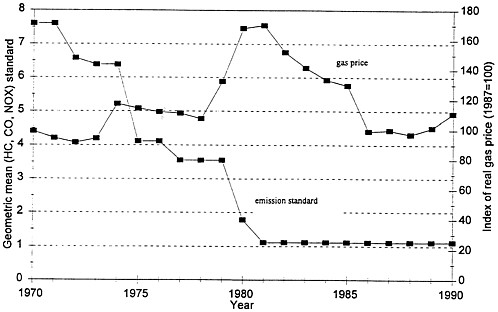
FIG. 1. Sources of change in the auto industry. Shows plots of emission standards and gas prices against time.
may discover that the reasons for the problems in the labor and capital equations require us also to modify the materials equation, so we continue to explore other approaches in our on-going research.
The materials demand equation that we estimate for automobile model j produced at plant p in time period t has several components. In our companion paper we discuss alternative specifications for these components, but here we only provide some intuition for the simple functional form that we use.
Since we are concerned that because labor and capital may be subject to long-term adjustment processes in this industry and a static cost minimizing assumption for them might be inappropriate, we consider a production function that is conditional on an arbitrary index of labor and capital. This index, which may differ with both product characteristics, to be denoted by x, and with time, or t, will be denoted by G(L, K, x, t). Given this index, production is assumed to be a fixed coefficient times materials use.
The demand for materials, M, is then a constant coefficient times output. That coefficient, to be denoted by c(xj, εpt, β), is a function of: product characteristics (xj), a plant-specific productivity disturbance (εpt), and a vector of parameters to be estimated (β). In this paper, we consider only linear input-output coefficients, i.e.,
c=xjβ+εp.
[1]
Finally, we allow for a proportional time-specific productivity shock, δt. This term captures changes in underlying technology and, possibly, in the regulatory environment. (In more complicated specifications it can also capture changes in input prices that result in input substitution.) The production function is then
[2]
Then, the demand for materials that arises from the variable cost of producing product j at plant p at time t is
Mjpt=δtc(xj, εpt, β)QJpt.
[3]
While we assume that average variable costs are constant (i.e., that the variable portion of input demand is linear in output), we do allow for increasing returns via a fixed component of cost. We denote the fixed materials requirement as µ. There may also be some fixed cost to producing more that one product at a plant. Specifically, let there be a set-up cost of ∆ for each product produced at a plant; we might think of this as a model change-over cost.c Let J(p) be the set of models produced by plant p and Jp be the number of them. Then total factor usage is given by
[4]
with Mjpt as defined in Eq. 3.
If we divide Eq. 4 through by plant output and rearrange, we obtain the equation we take to data
[5]
where ![]() is the weighted average
is the weighted average
[6]
Except for the proportional time-dummies, δ, Eq. 5 could be estimated by ordinary least squares (under appropriate assumptions on ε).d With the proportional δ, the equation is still easy to estimate by non-linear least squares.
Our results are preliminary in that they ignore a number of important economic and econometric issues. First, the plant and product outputs are used as weights in the construction of the right-hand-side variables in Eq. 5, and we have not accounted for the possible econometric endogeneity of output. There are assumptions that would justify treating output as exogenous, but they are not very convincing.e In calculating standard errors we ignore heteroskedasticity and the likely correlation of εpt across plants (due to, say, omitted product characteristics and the fact that the same products are produced at more than one plant) and over time (due to serially correlated plant productivities). Our functional forms allow for fixed costs, but no other form of increasing returns. Finally we do not engage in a more detailed exploration of substitution patterns between materials and labor or capital.f
Each of these issues is important and worthy of further exploration. In our on-going research we are examining the robustness of our results, and extending our models where it seems necessary.
The Data
We constructed our data set by merging data on the characteristics of automobile models with United States Bureau of the Census data on inputs and costs at the plants at which those models were assembled. The sources for most of the characteristics data were annual issues of the Automotive News Market Data Book (Crain Auto Group).g To determine which models were assembled at which plants we used data from annual issues of Wards Automotive Yearbook on assembly plant sourcing.h For each model year Wards publishes the quantity assembled of each model at each assembly plant. Because we did not have good data on the characteristics of trucks, we eliminated plants that assembled vans and trucks. We also eliminated plants that produced a significant number of automobile parts for final sale, because we had no way to separate out the cost of producing those parts.i
The Bureau of the Census data are is from the Longitudinal Research Data File, which, in turn, is constructed from information provided to the Annual Survey of Manufacturing (ASM) in non-census years, and information provided to the Census Of Manufacturing in census years (see ref. 15 for more information on the Longitudinal Research Data File). The ASM does not include quantity data, although the quintannual census does. All of the data (from both the ASM and the census) are on a calendar year basis.
Although the census data on costs are on a calendar year basis, the Ward’s data on quantities and the Automotive News data on characteristics are on a model year basis (and since the model year typically begins in August of the previous year, the number of vehicles assembled in a model year can differ significantly from those assembled in a calendar year). Thus, we needed a way of obtaining annual calendar year data on quantities.
Bresnahan and Ramey (16) used data on posted line speed, number of shifts per day, regular hours, and overtime hours at weekly intervals from issues of Automotive News to construct weekly posted output for most United States assembly plants from 1972 to 1982. We used their data to adjust the Ward’s data
Table 1. Characteristics of the sample
|
Year |
No. of plants |
Average quantity |
Average no. of models per plant |
|
1972 |
20 |
202,000 |
3.4 |
|
1973 |
21 |
196,000 |
2.4 |
|
1974 |
20 |
146,000 |
2.5 |
|
1975 |
21 |
130,000 |
2.7 |
|
1976 |
20 |
165,000 |
2.6 |
|
1977 |
19 |
198,000 |
2.6 |
|
1978 |
20 |
206,000 |
2.3 |
|
1979 |
21 |
184,000 |
2.3 |
|
1980* |
20 |
|
|
|
1981 |
22 |
155,000 |
2.7 |
|
1982 |
23 |
134,000 |
2.9 |
|
*Not published; census confidentiality. |
|||
to a calendar year basis.j We note that it is the absence of these data for the years 1984–1990 that limits our analysis to the years 1972–1982.
Table 1 provides characteristics of our sample. It covers about 50% of the total United States production of automobiles, with higher coverage at the end of the sample. The low coverage stems from our decision to drop the large number of plants producing both automobiles and light trucks or vans. There are about 20 active automobile assembly plants each year in our sample, and 29 plants that were active at some point during our sample period.k These plants are quite large. Depending on the year, the average plant assembles 130,000– 202,000 automobiles, and employs 2,814–4,446 workers (about 85% of them production workers). Note that the average plant produces 2.4–3.4 distinct models each year.
Table 2 provides annual information on the average (across plants) materials input per vehicle assembled and the unit values of these vehicles. The materials series is constructed as the costs of parts and materials (engines, transmissions, stamped sheet metal, etc.), as well as energy costs, all deflated by a price index for materials purchased by SIC 3711 (Motor Vehicles and Car Bodies), constructed by Wayne Gray and Eric Bartelsman (see the National Bureau of Economic Research data base).l Because we use an industry and factor specific price deflater, we interpret the materials series as an index of real materials input. The unit values are the average of the per vehicle price received by the plants for the vehicles assembled by those plants deflated by the gross domestic product deflater.
This measure of materials input represents the lion’s share of the total cost of the inputs used by these assembly plants; on average, the share of materials in total costs was about 85%, with most of the balance being labor cost.m Material costs per vehicle were fairly constant during the first half of the 1970s, but moved upwards after 1975, with a sharp jump in 1982. As one might expect, these cost trends were mirrored in the unit value numbers.
Of course the characteristics of the vehicles produced also changed over this period. Annual averages for many of these characteristics are provided, for example, in ref. 7, although
|
g |
The initial characteristics data base was graciously provided by Ernie Berndt. It was then updated and extended first by Berry et al. (7) and then by us (see below). More detail on this data base can be found in ref. 7. |
|
h |
An initial data set based on Wards Automotive Yearbook was graciously provided to us by Joshua Haimson and we simply updated and extended it. |
|
i |
In the census years (1972, 1977, 1982) we can look at the value of shipments by type of product. Automobiles are over 99% of the value of shipments for all but one of our plants. Other products made up about 4% of the value of shipments for that plant in 1982. |
|
j |
These data were graciously provided to us by Valerie Ramey. We use it to allocate the Ward’s data across weeks. We then aggregate the weekly data to the calendar year quantities needed for the cost analysis. |
|
k |
We did not use the information from the first year of a plant that started up during our sample period, or the information from the last year of a plant that exited during this period. This was to avoid modeling any additional costs to opening up or shutting down a plant. Of the 29 plants that operated at some point in our 10-year period, 6 exited before 1983. |
|
l |
Energy costs are a very small fraction of material costs, under 1%, throughout the period. |
Table 2. Materials use and unit values
|
Year |
Cost of materials |
Cost per unit value |
Cost share materials |
|
1972 |
6,444 |
8,901 |
0.86 |
|
1973 |
6,636 |
8,847 |
0.85 |
|
1974 |
6,512 |
8,727 |
0.84 |
|
1975 |
6,316 |
8,652 |
0.85 |
|
1976 |
6,470 |
9,009 |
0.86 |
|
1977 |
6,757 |
9,320 |
0.87 |
|
1978 |
6,745 |
9,286 |
0.86 |
|
1979 |
6,694 |
9,724 |
0.85 |
|
1980* |
|
||
|
1981 |
6,879 |
9,438 |
0.84 |
|
1982 |
7,493 |
10,672 |
0.85 |
|
*Not published; census confidentiality. |
|||
those numbers are for the universe of cars sold, rather than for our production sample. In our sample, the number of cars with air conditioning (AC) as standard equipment begins at near zero near the beginning of the sample and increases to almost 15% by 1982. Average mpg, discussed further below, increases from 14 to about 23, while average horsepower declines from about 148 to near 100. The weight of cars also decreases from about 3800 to 2800 pounds. Note that the fact that these large changes in x characteristics occurred implies that we should not interpret the increase in the observed production costs (or in observed price) per vehicle as an increase in the cost or price ofa “constant quality” vehicle.
As noted, in addition to characteristics valued directly by the consumer (such as horsepower, size, or mpg), we are also interested in how the technological characteristics of a car (particularly those that effected emissions and fuel efficiency) changed over time and affected costs. In our sample period, the automobile companies adopted a number of new technologies in response to both lower emission standards and higher gas prices. Bresnahan and Yao (17) have collected detailed data on which cars used which technology.n In particular, using the Environmental Protection Agency’s Test Car List, they tracked usage of five technologies: no special technology (a baseline), oxidation catalysts (i.e., catalytic converters), three-way catalysts, three-way closed-loop catalysts, and fuel injection. Census confidentiality requirements prohibit us from presenting the proportion of vehicles in our sample using each of these technologies, so Table 3 uses publicly available data to compute the fraction of car models built by United States producers using each technology in each model year. The baseline technology was used in virtually all models until the 1975 model year, at which time most models shifted to catalytic converters. The catalytic converters began to be displaced by the more modern technologies in the 1980 model year, and by 1981 they had been displaced in over 80% of the models.
Results from the Production Data
Table 4 presents baseline estimates of the materials demand equation. The right-hand-side variables include: the term 1/Q, whose coefficient determines fixed costs; the term J/Q, whose coefficient determines model changeover costs; the product characteristics (the x variables); and, in the right-most specification, the time-specific parameters (the δt), which shift the variable component of the materials cost over time (see Eq. 5).
In many studies, the parameters on the x variables would be the primary focus of analysis. However, in the present context they are largely included as a set of controls that allow us to get more accurate estimates of the shifts in material costs over time (i.e., of the δt). The difference between the two sets of results presented in Table 4 is that the second set includes these δt, whereas the first set does not. The sum of square residuals reported at the bottom of the table indicate that these time effects are jointly significant at any reasonable level of significance.
The estimates of the materials demand equation do not provide a sharp indication of the importance of model changeover costs, or of fixed costs (at least after allowing for the time effects), or of a constant cost that is independent of the characteristics of the car. However, most of the product characteristics have parameter estimates that are economically and statistically significant. For example, the coefficients on AC indicate that having AC as standard equipment increases per car materials costs by about $2600 (in the specification with the δt) and by about $3600 (in the specification without). We think that the AC dummy variable proxies for a package of “luxury standard equipment,” so the large figures here are not surprising. A 1 mpg increase in fuel efficiency is estimated to raise costs in the range of $80–$160, whereas a 1 pound increase in weight increases costs by around $1.30–$1.50.
Table 4 presents estimates of ln(δ), not levels, so the coefficients have the approximate interpretation of percentage changes over the base year of 1972. In the early years these coefficients are not significantly different from zero, but they become significant in 1977 and stay so. There appears to be a clear upward trend, with apparent jumps in 1977 and 1980.
We now come back to the question of how well cost changes correlate with changes in emissions standards. Emissions requirements took two jumps, one in 1975 (when they were tightened by about 40%) and one in 1980, when an even greater tightening occurred. Table 4 finds a jump in production costs in 1980, but not in 1975.
One possible explanation is that early adjustments to the fuel emissions requirement were crude, but relatively inexpensive and came largely at the cost of “performance” (a characteristic that may not be adequately captured by our observed characteristics). Later technologies, such as fuel injection, may have been more costly in dollar terms, but less so in terms of performance.
We use the technology variables described in Table 3 to study the effect of technology in more detail. These variables are potentially interesting because, although there is no cross-sectional variation in fuel efficiency and emissions requirements, there is cross-sectional variation in technology. Thus, they might let us differentiate between the impacts on costs of other time specific variables (e.g., input prices), and the new technologies that were at least partially introduced as responses to the emissions requirements. In particular, we would like to know if the technology variables can help to explain the increasing series of time dummies found in Table 5.
Let τjt be a vector of indicator variables for the type of technology used in model j at time t. We introduce these technology indicators as a further proportional shift term in the estimation equation. In particular, we alter Eq. 3 so that the variable portion of the materials demand for product j at time t is
Mjpts=δtexp(τjtγ)c(xj, εpt, β)Qjpt.
[7]
where γ is the vector of parameters giving the proportionate shift in marginal costs associated with the different technologies. Just as one of the δs is normalized to one, so we normalize the γ associated with the baseline technology to
Table 3. Technology variables (proportion of sample)
|
Model year |
Baseline |
Catalytic converter |
3-way converter |
Open loop |
Fuel injection |
|
1972 |
1 |
0 |
0 |
0 |
0 |
|
1973 |
1 |
0 |
0 |
0 |
0 |
|
1974 |
1 |
0 |
0 |
0 |
0 |
|
1975 |
0.15 |
0.84 |
0 |
0 |
0.01 |
|
1976 |
0.19 |
0.80 |
0 |
0 |
0.01 |
|
1977 |
0.09 |
0.89 |
0 |
0 |
0.02 |
|
1978 |
0.03 |
0.95 |
0 |
0 |
0.02 |
|
1979 |
0 |
0.98 |
0 |
0.01 |
0.02 |
|
1980 |
0 |
0.86 |
0 |
0.08 |
0.06 |
|
1981 |
0 |
0.18 |
0.20 |
0.59 |
0.03 |
|
1982 |
0 |
0.16 |
0.38 |
0.44 |
0.02 |
|
1983 |
0 |
0.05 |
0.31 |
0.37 |
0.27 |
zero. Note that we can separately identify the δs and the γs because of the cross-sectional variation in technologies.
Table 5 gives some results from estimating the materials equation with the technology variables included. The first is exactly as in Eq. 7. From prior knowledge and from this first regression, we believe that simple catalytic converters may be relatively cheap, whereas the others may be more expensive. Therefore, as a second specification, we constrain the γ for catalytic converters (technology 1) to be equal to the baseline technology.
We see that the technology parameters, the γs, generally have the expected sign and pattern. In the first specification, the γ associated with simple catalytic converters is estimated at about zero, whereas the others are positive, though not statistically significantly so, and increasing as the technology becomes more complex. In the second specification (with γ1 ≡ 0) the coefficients on technology are individually significant and have the anticipated, increasing pattern.
Recall from Table 3 that simple catalytic converters began to be used at the time of the first tightening of emissions standards, and were used almost exclusively between 1975 and 1979 (inclusive). In 1980, when the emissions standard were tightened for the second time, the share of catalytic converters began to fall, and by 1981 the simple catalytic converter technology had been abandoned by over 80% of the models.
Thus, the small cost coefficient on catalytic converters is consistent with the small estimate of the change in production costs following the first tightening in emissions requirements found in Table 4, whereas the larger cost effects of the later technologies helps explain Table 4’s estimated increase in production costs following the second tightening of the emissions standards in 1980. Indeed, once we allow for the technology classes as in Table 5, the time effects (the δs) are only marginally significant, and there is no longer a distinct upward trend in their values.
As an outside check on our results, we note that the Bureau of Labor Statistics publishes an adjustment to the vehicle component of the Consumer Price Index for the costs of meeting emissions standards [the information is obtained from questionnaires to plant managers; see the Report on Quality Changes for Model Passenger Cars (EPA), various years]. After taking out their adjustments for retail margins and deflating their series, we find that it shows a sum total of $71 in emissions adjustment costs between 1971 and 1974 and then an increment of $176 in 1975. The Bureau of Labor Statistics’ series then increases by only $56 between 1975 and 1979, but jumps by $632 between 1979 and 1982. Table 5 estimates very similar numbers. Note however that some of the costs of the new technologies that we are picking up may have been partially offset by improved performance characteristics not captured in
Table 4. Results from the materials equation
Table 5. Materials demand with technology effects
|
Variable |
|
Estimate |
|
Standard error |
Estimate |
|
Standard error |
|
1/Q |
µ |
16.6 m |
|
14.7 m |
17.2 m |
|
14.4 m |
|
J/Q |
∆ |
–1.3 m |
5.9 m |
–2.7 m |
5.7 m |
||
|
Constant |
β0 |
–689.2 |
1207 |
–608.2 |
1143 |
||
|
AC |
β1 |
2138.1 |
279.3 |
2172 |
261.7 |
||
|
mpg |
β2 |
86.4 |
32.6 |
85.8 |
31.2 |
||
|
hp |
β3 |
4.5 |
3.7 |
4.4 |
3.7 |
||
|
wt |
β4 |
1.34 |
0.26 |
1.33 |
0.25 |
||
|
τ |
γ |
|
|||||
|
Catalytic converter |
γ1 |
–0.01 |
0.12 |
0 |
— |
||
|
Three-way |
γ2 |
0.14 |
0.15 |
0.15 |
0.08 |
||
|
Closed loop |
γ3 |
0.20 |
0.15 |
0.21 |
0.08 |
||
|
Fuel injection |
γ4 |
0.28 |
0.14 |
0.29 |
0.07 |
||
|
t |
ln(δ) |
|
|||||
|
1973 |
|
0.02 |
0.04 |
0.02 |
0.04 |
||
|
1974 |
0.00 |
0.06 |
–0.00 |
0.04 |
|||
|
1975 |
–0.02 |
0.12 |
–0.02 |
0.04 |
|||
|
1976 |
0.02 |
0.13 |
–0.01 |
0.04 |
|||
|
1977 |
0.09 |
0.13 |
0.08 |
0.04 |
|||
|
1978 |
0.11 |
0.13 |
0.11 |
0.04 |
|||
|
1979 |
0.11 |
0.13 |
0.10 |
0.04 |
|||
|
1980 |
0.12 |
0.14 |
0.11 |
0.06 |
|||
|
1981 |
–0.01 |
0.15 |
–0.02 |
0.09 |
|||
|
1982 |
0.02 |
0.15 |
0.02 |
0.08 |
|||
|
ssq |
|
113.6 m |
|
113.6 m |
|
||
|
The dependent variable is material cost per car in 1983 dollars, and there are 227 observations. An m after a figure indicates millions of dollars. The total sum of squares is 559.8 m. For abbreviations see Table 4. |
|||||||
The Fuel Efficiency of the New Car Fleet
Recall that gas prices increased sharply in 1974 and then again between 1978 and 1980. They trended downward from 1982. Table 6 (from the ref. 24 data set) shows how the median fuel efficiency of new car sales has changed over time. There was very little response of the mediano of the mpg of new car sales to the gas price hike of 1973 until 1976. As discussed in Pakes et al. (18), this is largely because more fuel efficient models were not introduced until that time, and the increase in gas prices had little effect on the distribution of sales among existing models. The movement upward in the mpg of new car sales that began in 1976 continued, though at only a modest rate, until 1979. Between 1979 and 1983 there was a more striking rate of improvement in this distribution. After 1983, the distribution seems to trend slowly downward with the gas price.
These trends are replicated, though in somewhat different intensities and years, in the downward movements in both the weight and horsepower distributions of the cars marketed. There is, then, the possibility that the increase in the mpg of cars was mostly at the expense of the weight and horsepower of the models marketed, i.e., there was no change in the mpg for given horsepower-weight (hp/wt) classes.
To investigate this possibility we calculated a “divisia” index of mpg per hp/wt class. That is, first we divided all models into nine hp/wt classes,p then calculated the annual change in the mpg in each of these classes, and then took a weighted average of those changes in every year; the weights being the fraction of all models marketed that were in the class in the base year for which the increase was being calculated. This index is given in column 2 of Table 6. It grew rapidly in most of the period between 1976 and 1983 (the average rate of growth was 2.85% per year), though there was different behavior in different subperiods (the index fell between 1978 and 1980 and grew most rapidly in 1976 and 1977).
We would expect this index to increase if either of the firms moved to a different point on a given cost surface, being willing to incur higher production costs for more fuel efficient cars, or if the gas price hike induced technological change that enabled firms to produce more fuel efficient cars at no increase in cost. Comparing the movements in the mpg index in Table 6 to the time dummies estimated in Table 5, we see little correlation between the mpg index and our estimates of the δt.q We therefore look at the possibility that the mpg index increases were generated by induced technological change.r
Innovation
As noted, another route by which changes in the environment can affect the automobile industry is through induced innovation. Table 3 showed how some new technologies have been introduced over time. The table shows that the simple catalytic converter was introduced immediately after the new fuel emission standards in 1975, and lasted until replaced by more modern technologies beginning in 1980.
Other than looking at specific technologies, it is very difficult to measure either innovative effort or outcomes, and hence to judge either the extent or the impacts of induced innovation. Perhaps the best we can do is to look at those patent appli-
|
o |
Indeed, we have looked at the entire distribution of the mpg of new car sales and its movements mimic those of the median. |
|
p |
We divided all models marketed into three equally sized weight classes, generating in this way cutoff points for large, medium, and small weight classes. We then did the same for the horsepower distribution. We placed each model into one of the nine hp/wt classes determined by the horsepower and weight cutoffs we had determined. |
|
q |
On the other hand there is some correlation between the mpg index and the time dummies in Table 4, suggesting that the technologies we describe in Table 3 might also have increased fuel efficiency |
|
r |
We have also examined whether we could pick up changes in the mpg coefficient over time econometrically. However, once we started examining changes in coefficients over time there was too much variance in the point estimates to do much in the way of intertemporal comparisons. |
Table 6. Evolution of fuel efficiency
cations that were eventually granted in the three subclasses of the international patent classification that deal with combustion engines (F02B, F02D, and F02M: Internal Combustion Engines, Controlling Combustion Engines, and Supplying Combustion Engines with Combustible Materials or constituents Thereof). A time series of the patents in these subclasses is plotted in Fig. 2.
That series indicates that the timing of the changes in the number of patent applications in these classes is remarkably closely related to the timing of both the gas price changes and the changes in emissions standards. In the 10-year period between 1959 and 1968 the annual sum of the number of patent applications in these classes stayed almost constant at 312 (it varied between 258 and 346). There was a small jump in 1969 to 416, and between 1969 and 1972 (which corresponds to the period when emissions standards were introduced) the number of patents averaged 498. A rather dramatic change occurred in the number of patents applied for in these classes after the first oil price shock in 1973/74 (an increase to 800 in 1974), and the
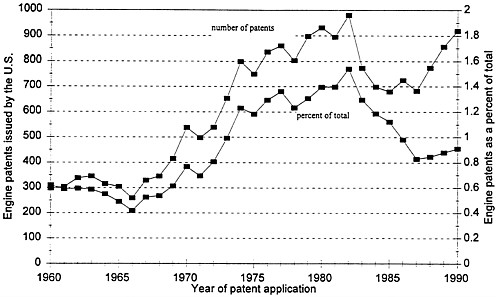
FIG. 2. Patents in engine technologies plotted against time.
average number between 1974 and 1983 was 869. This can be divided into an average of 810 between 1974 and the second oil price shock in 1979, and an average of 929 between 1979 and 1983. These later jumps in applications in the combustion engine related classes occurred at the same time as the total United States patent applications fell, making the increase in patenting activity on combustion engines all the more striking.
It seems then that the gas price shocks, and to a possibly lesser extent the regulatory changes, induced significant increases in patent applications. Of course there is likely to be a significant and variable lag between these applications and the subsequent embodiment of the patented ideas in the production processes of plants. Moreover, very little is known about this lag. What does seem to be the case is that patent applications and research and development expenditures have a large contemporaneous correlation (see ref. 19). However, the attempts at estimating the lag between research and development expenditures and subsequent productivity increases have been fraught with too many simultaneity and variability problems for most researchers (including ourselves in different incarnations) to come to any sort of reliable conclusion about its shape.
Conclusions
In this paper we provide some preliminary evidence on the impact of regulatory and gas price changes on production costs and technological change. We find that, after controlling for product characteristics, costs moved upwards in our period (1972–1982) of rapidly changing gas prices and tightened emissions standards.
When we introduce dummy variables for technology classes we find that the simple catalytic converter technology that was introduced with the first tightening of emission standards did not have a noticeable impact on costs, but the more advanced technologies that were introduced with the second tightening of emissions standards did. Moreover, the introduction of the technology dummies eliminates the shift upwards in costs over time. Thus, the increase in costs appear to be related to the adoption of new technologies that resulted in cleaner, and perhaps more fuel efficient, cars.
The fuel efficiency of the new car fleet began increasing after 1976, and continued this trend until the early 1980s, after which it, with the gas price, slowly fell. Our index of mpg per hp/wt class also began increasing in 1976 and, at least after putting in our technology variables, its increase was not highly
correlated with the index of annual costs that we estimate. Also, patent applications in patent classes that deal with combustion engines increased dramatically after both increases in gas prices. These latter two facts provide some indication that gas price increases induced technological change, which enabled an increase in the fuel efficiency of new car models with only moderate, if any, increases in production costs.
In future work we hope to provide a more detailed analysis of these phenomena, as well as integrate (perhaps improved versions) of our hedonic cost functions with an analysis of the demand-side of the market (as in ref. 7). This ought to enable us to obtain a deeper understanding of the automobile industry and its likely responses to various changes in its environment.
We thank the participants at the National Academy of Sciences conference on Science and the Economy, particularly to Dale Jorgenson, and to Zvi Griliches, Jim Levinsohn, and Bill Nordhaus, for helpful comments. Maria Borga, Deepak Agrawal, and Akiko Tamura provided excellent research assistance. We gratefully acknowledge support from National Science Foundation Grants SES-9122672 (to S.B., James Levinsohn, and A.P.) and SBR-9512106 (to A.P.) and from Environmental Protection Agency Grant R81–9878–010.
1. Dewees, D.N. (1974) Economics and Public Policy: The Automobile Pollution Case (MIT Press, Cambridge, MA).
2. Toder, E.J., Cardell, N.S. & Burton, E. (1978) Trade Policy and the U.S. Automobile Industry (Praeger, New York).
3. White, L.J. (1982) The Regulation of Air Pollutant Emissions from Motor Vehicles (American Enterprise Institute, Washington, DC).
4. Abernathy, W.J., Clark, K.B. & Kantrow, A.M. (1983) Industrial Renaissance: Producing a Competitive Future for America (Basic Books, New York).
5. Crandall, R., Gruenspecht, T., Keeler, T. & Lave, L. (1986) Regulating the Automobile (Brookings Institution, Cambridge, MA).
6. Aizcorbe, A., Winston, C. & Friedlaender, A. (1987) Blind Intersection? Policy and the Automobile Industry (Brookings Institution, Washington, DC).
7. Berry, S., Levinsohn, J. & Pakes, A. (1995) Econometrica 60, 889–917.
8. Havenrich, R., Marrell, J. & Hellman, K. (1991) Light-Duty Automotive Technology and Fuel Economy Trends Through 1991: A Technical Report (EPA, Washington, DC).
9. Lancaster, K. (1971) Consumer Demand: A New Approach (Columbia Univ. Press, New York).
10. Court, A. (1939) The Dynamics of Automobile Demand (General Motors Corporation, Detroit), pp. 99–117.
11. Griliches, Z. (1961) The Price Statistics of the Federal Government (NBER, New York).
12. Bresnahan, T. (1987) J. Ind. Econ. 35, 457–482.
13. Feenstra, R. & Levinsohn, J. (1995) Rev. Econ. Studies 62,19–52.
14. Friedlaender, A. R, Winston, C. & Wang, K. (1995) RAND 14,1–20.
15. McGuckin, R. & Pascoe, G. (1988) Surv. Curr. Bus. 68, 30–37.
16. Bresnahan, T. & Ramey, V. (1994) Q.J. Econ. 109, 593–624.
17. Bresnahan, T.F. & Yao, D.A. (1985) RAND 16, 437–455.
18. Pakes, A., Berry, S. & Levinsohn, J. (1993) Am. Econ. Rev. Paper Proc. 83, 240–246.
19. Pakes, A. & Griliches, Z. (1980) Econ. Lett. 5, 377–381.


