
This paper was presented at a colloquium entitled “Earthquake Prediction: The Scientific Challenge,” organized by Leon Knopoff (Chair), Keiiti Aki, Clarence R.Allen, James R.Rice, and Lynn R.Sykes, held February 10 and 11, 1995, at the National Academy of Sciences in Irvine, CA.
Scale dependence in earthquake phenomena and its relevance to earthquake prediction
KEIITI AKI
Department of Earth Sciences, University of Southern California, Los Angeles, CA 90089–0740
ABSTRACT The recent discovery of a low-velocity, low-Q zone with a width of 50–200 m reaching to the top of the ductile part of the crust, by observations on seismic guided waves trapped in the fault zone of the Landers earthquake of 1992, and its identification with the shear zone inferred from the distribution of tension cracks observed on the surface support the existence of a characteristic scale length of the order of 100 m affecting various earthquake phenomena in southern California, as evidenced earlier by the kink in the magnitude-frequency relation at about M3, the constant corner frequency for earthquakes with M below about 3, and the source-controlled fmaxof 5–10 Hz for major earthquakes. The temporal correlation between coda Q−1and the fractional rate of occurrence of earthquakes in the magnitude range 3–3.5, the geographical similarity of coda Q−1and seismic velocity at a depth of 20 km, and the simultaneous change of coda Q−1and conductivity at the lower crust support the hypotheses that coda Q−1may represent the activity of creep fracture in the ductile part of the lithosphere occurring over cracks with a characteristic size of the order of 100 m. The existence of such a characteristic scale length cannot be consistent with the overall self-similarity of earthquakes unless we postulate a discrete hierarchy of such characteristic scale lengths. The discrete hierarchy of characteristic scale lengths is consistent with recently observed logarithmic periodicity in precursory seismicity.
A starting point for the science of earthquake prediction may be to find what seismogenic structures control the earthquake processes. We have invented jargon to describe structures such as asperities, barriers, breakdown zones, locking depth, and the brittle-ductile transition zone. If there is any distinct structure controlling earthquake processes, it should show up as scale-dependent phenomena—namely, departure from self-similarity. However, if all earthquakes are put together as shown, for example, in the seismic moment-source dimension relation summarized by Abercrombie and Leary (1) the self-similarity roughly holds over the range of source dimension from 10 cm to 100 km, telling us that there may be no universal structure controlling earthquake processes.
There is still a hope that we may find such a controlling structure if we focus our attention on a specific fault zone or a specific seismic region and use techniques with higher resolution and accuracy. To explain why I have such a hope, I shall first describe my encounters with scale-dependent earthquake phenomena in the past two decades.
After I found (2) that the ω-squared scaling law with a constant stress drop independent of magnitude explains the observed source spectral ratios (3) and resolves inconsistencies between surface wave magnitude and body wave magnitude, a natural follow-up was to determine the scaling law in various parts of the earth and map the stress drop globally. During the course of this work, we (4) found that very often the shape of the seismic spectrum does not obey the ω-squared scaling law but stays the same over a considerable range (2–3 orders) of seismic moment. This means that the corner frequency stays at a constant value and stress drop decreases with decreasing magnitude. Rautian et al. (5) have studied the same problem independently in the former Soviet Union and discovered the same phenomena. The existence of a constant corner frequency must mean that there is a unique scale length governing the earthquake phenomena. The value of the constant corner frequency varied from place to place in the range from a few to >10 Hz.
My next encounter with the unique scale length was when Papageorgiou and I (6) were trying to predict the strong motion acceleration power spectra by using the specific barrier model. We found that the shape of the acceleration power spectrum is flat for frequencies higher than the subevent corner frequency, but the flat part is limited to the fmax [term coined by Hanks (7)] beyond which the spectrum sharply decays with increasing frequency (6). We found that fmax is in the range of a few to 10 Hz and shows a slight dependence on magnitude. It was very natural for me to suspect a tie between the constant corner frequency for small earthquakes and the fmax for large earthquakes. Papageorgiou and Aki (6) attributed the origin of fmax to the cohesive zone of an earthquake fault.
My third encounter with a unique scale length associated with earthquakes occurred when Okubo and I (8) were measuring the fractal dimension of the San Andreas fault with the map of fault traces published by the U.S. Geological Survey. We found that there is an upper bound length beyond which the fault ceases to be fractal, and it ranges from a few hundred meters to a kilometer, in agreement with the size of the cohesive zone inferred from fmax.
My fourth encounter with the unique scale length is the finding of a kink in the frequency magnitude relation at about M=3 from the recordings made at a borehole station within the Newport-Inglewood fault zone in southern California (9). The size of an M=3 earthquake is a few hundred meters, which roughly corresponds to the size of the cohesive zone estimated from fmax.
My most intriguing encounter with a characteristic scale length, however, was the very strong temporal correlation between coda Q−1 and the fractional rate of earthquakes with magnitudes in a certain range (10, 11). On the other hand, the most direct confirmation of the fault zone structure with a characteristic width came from the observation of the seismic guided waves trapped in the fault zone of the Landers earthquake (12). In the present paper, I focus on these latter two subjects—namely, the coda Q and fault zone trapped
The publication costs of this article were defrayed in part by page charge payment. This article must therefore be hereby marked “advertisement” in accordance with 18 U.S.C. §1734 solely to indicate this fact.
modes—in order to infer the interrelations between fault zone structures and earthquake processes.
Three-Dimensional Structure of the 1992 Landers Earthquake Fault Zone
As far as I know, seismic guided waves trapped in a fault zone were first discovered in a three-dimensional vertical seismic profiling experiment conducted in the area surrounding a borehole drilled into the fault zone of the Oroville, California, earthquake of 1975 (13, 14). Records of borehole seismographs placed near the fault zone showed an unusually long-period wave train when the seismic source (a thumper) crossed the fault zone at the surface. The characteristic waveform was attributed to a Love wave-type mode trapped in a low-velocity, low-Q zone. Similar trapped modes were also identified in some of the borehole seismograms obtained at the San Andreas fault near Parkfield, California (15).
The Landers, California, earthquake of 1992 offered a wealth of data for studying various aspects of fault zone trapped modes. By comparing the observed waveform with the synthetic waveform for a low-velocity, low-Q zone, Li et al. (12) estimated a fault zone width around 180 m, with shear velocity of 2.0–2.2 km/sec and a Q value of ≈50.
Interestingly, a similar estimate of fault zone width was made in an entirely different study. From a detailed study of tension cracks on the surface, Johnson et al. (16) concluded that the Landers fault rupture is not a distinct slip across a fault plane but rather a belt of localized shearing spread over a width of 50–200 m. They suggested that this might be a common structure of an earthquake fault, which might have been unrecognized previously because the shearing is small, and surficial material is usually not as brittle as in the Landers area. We identify this shear zone with the low-velocity, low-Q zone found from the trapped modes because their widths are virtually the same. Since the trapped modes were observed from aftershocks with focal depths of >10 km, we conclude that the shear zone found by Johnson et al. (16) extends to the same depth.
More recently, Li et al. (17) conducted an active experiment by shooting explosives in the Landers fault zone. They successfully recorded not only the direct trapped modes but also the reflection from the bottom of the fault zone at a depth of ≈10 km.
A CALCRUST (California Consortium for Crustal Studies) seismic reflection line was shot in the area of a similar geological setting as the Landers epicentral area. The resultant CDP time section (18) clearly presents the transition from nonreflective upper crust to strongly reflective lower crust, which has been identified with the ductile part of the crust globally (19). The transition occurs at a depth of 10 km, in agreement with the bottom depth of the low-velocity, low-Q zone found from the trapped modes. Thus, combining all these observations, we have strong evidence supporting the hypothesis that the shear zone found near the surface extends to the top of the ductile part of the crust.
Furthermore, if we identify the low-velocity, low-Q zone with the breakdown zone of the specific barrier model (6), the source of controlled fmax will be of the order of rupture velocity divided by the zone width (≈10 Hz), in agreement with our observations.
In any case, the shear zone with a width of 200 m can serve only as the micromechanism of earthquakes with a fault length much longer than, say, 1 km. Thus, earthquakes associated with this fault zone must be scale dependent, and we should observe a departure from self-similarity.
Let us now turn to recent results from coda Q−1 studies relevant to the subject of the present paper. Since coda waves are not explained in any existing seismology textbook, I shall first briefly describe what they are.
Seismic Coda Waves
When an earthquake occurs in the earth, seismic waves are propagated away from the source. After P waves, S waves, and various surface waves are gone, the area around the seismic source is still vibrating. The amplitude of vibration is uniform in space, except for the local site effect, which tends to amplify the motion at soft soil sites compared to hard rock sites. These residual vibrations are called seismic coda waves and they decay very slowly with time. The rate of decay is roughly the same independent of the locations of seismic source and recording station, as long as they are located in a given region.
The closest phenomenon to this coda wave is the residual sound in a room, first studied by Sabine (20). If someone shoots a gun in a room, the sound energy remains for a long time because of incoherent multiple reflections. This residual sound has a very stable, robust nature similar to seismic coda waves, independent of the locations where the gun was shot or where the sound in the room was recorded. The residual sound remains in the room because of multiple reflections at the rigid wall, ceiling, and floor of the room. Since we cannot hypothesize any room-like structure in the earth, we attribute seismic coda waves to backscattering from numerous heterogeneities in the earth. We may consider seismic coda as waves trapped in a random medium.
The seismic coda waves from a local earthquake can be best described by the time-dependent power spectrum P(ω|t), where ω is the angular frequency and t is the time measured from the origin time of the earthquake. P(ω|t) can be measured from the squared output of a bandpass filter centered at frequency ω or from the squared Fourier amplitude obtained from a time window centered at t. The most extraordinary property of P(ω|t) is the simple separability of the effects of seismic source, propagation path, and recording site response expressed by the following equation. The coda power spectrum Pij(ω|t) observed at the ith station due to the jth earthquake can be written as
Pij(ω|t)=Sj(ω) Ri(ω) C(ω|t), [1]
for t greater than about twice the travel time of S waves from they jth earthquake to the ith station. Eq. 1 means that Pij(ω|t) can be written as a product of a term that depends only on the earthquake source, a term that depends only on the recording site, and a term common to all the earthquakes and recording sites in a given region.
The above property of coda waves expressed by Eq. 1 was first recognized by Aki (21) for aftershocks of the Parkfield, California, earthquake of 1966. The condition that Eq. 1 holds for t greater than about twice the travel time of S waves was found by the extensive study of coda waves in central Asia by Rautian and Khalturin (22). Numerous investigators demonstrated the validity of Eq. 1 for earthquakes around the world, as summarized in a review article by Herraiz and Espinosa (23). In general, Eq. 1 holds more accurately for a greater lapse time t and for higher frequencies (e.g., see ref. 24). Coda waves are a powerful tool for seismologists because Eq. 1 offers a simple means to separate the effects of source, path, and recording site. The equation has been used for a variety of practical applications, including mapping of the frequency-dependent site amplification factor (e.g., see ref. 25), discrimination of quarry blasts from earthquakes (24), the single station method for determining frequency-dependent attenuation coefficients (26), and normalizing the regional seismic network data to a common source and recording site condition (27).
In the following, I focus on the common decay function C(ω|t) on the right side of Eq. 1. I first introduce coda Q to characterize C(ω|t) in the framework of single-scattering theory and then summarize the current results on what the
coda Q is in terms of scattering attenuation and intrinsic absorption. Then, I will survey the spatial and temporal variation in coda Q−1 and describe how they are related to earthquake processes in the lithosphere.
Introducing Coda Q (or Coda Q−1)
The first attempt to predict the explicit form of P(ω|t) for a mathematical model of earthquake source and earth medium was made by Aki and Chouet (28). Their models were based on the following assumptions.
-
Both primary and scattered waves are S waves.
-
Multiple scatterings are neglected.
-
Scatterers are distributed randomly with a uniform density.
-
Background elastic medium is uniform and unbounded.
Assumption i has been supported by various observations, such as the common site amplification (29) and the common attenuation (26) between S waves and coda waves. It is also supported theoretically because the S to P conversion scattering due to a localized heterogeneity is an order of magnitude smaller than the P to S scattering as shown by Aki (30) with the reciprocal theorem. Zeng (31) showed that the above difference in conversion scattering between P to S and S to P leads to the dominance of S waves in the coda.
Since the observed P(ω|t) is independent of the distance between the source and receiver, we can simplify the problem further by colocating the source and receiver. Then, we find (ref. 28; see also ref. 32 for more detailed derivation) that
P(ω|t)=β/2·g(π)|ϕo(ω|βt/2)|2, [2]
where β is the shear wave velocity, g(θ) is the directional scattering coefficient, and ϕo(ω|r) is the Fourier transform of the primary waves at distance r from the source. g(θ) is defined as 4π times the fractional loss of energy by scattering per unit travel distance of primary waves and per unit solid angle at the radiation direction θ measured from the direction of primary wave propagation.
Aki and Chouet (28) adopted the following form for |ϕo(ω|r)|.
|ϕo(ω|r)|=|S(ω)|r−1exp(−ωr/(2βQc)), [3]
where |S(ω)| is the source spectrum, r−1 represents the geometrical spreading, and Qc is introduced to express the attenuation. Combining Eqs. 2 and 3, and including the attenuation of scattered waves, we have
[4]
Qc is called coda Q, and Qc−1 is called coda Q−1.
The measurement of coda Q according to Eq. 4 is very simple. Coda Q−1 is the slope of straight line fitting the measured ln(t2P(ω|t)) vs. ωt. Since there is a weak but sometimes significant dependence of the slope on the time window for which the fit is made, it has become a necessary routine to specify the time window for each measured coda Q−1.
Because of the simplicity of measurement of coda Q−1, its geographical variation over a large area as well as its temporal variation over a long time can be studied relatively easily. Before presenting those results, however, we need to clarify the physical meaning of coda Q−1.
Physical Meaning of Coda Q−1
The physical meaning of coda Q−1 has been debated for almost 20 years. Within the context of the single scattering theory, coda Q−1 appears to represent an effective attenuation including both absorption and scattering loss. This idea prevailed for some time after Aki (26) found a close agreement between coda Q−1 and Q−1 of S waves measured in the Kanto region, Japan. On the other hand, numerical experiments by Frankel and Clayton (33), laboratory experiments by Matsunami (34), and theoretical studies including multiple scattering effects (e.g., ref. 35) concluded that the coda Q−1 measured from the time window later than the mean free time (mean free path divided by wave velocity) should correspond only to the intrinsic absorption and should not include the effect of scattering loss. The debates concerning this issue were summarized by Aki (36).
To resolve the above issue, attempts have been made to separately determine the scattering loss and the intrinsic loss in regions where coda Q−1 has been measured. For this purpose, it is necessary to include multiple scattering in the theoretical model, either by the radiative energy transfer approach (37) or by the inclusion of several multiple-path contributions to the single-scattering model (38). Recently, Zeng et al. (39) demonstrated that all these approaches can be derived as approximate solutions of the following integral equation for the seismic energy density E(x, t) per unit volume at location r and at time t due to an impulsive point source applied at χo at t=0.
[5]
where the symbols are defined as follows: E(x, t), seismic energy per unit volume at x and t; β, velocity of wave propagation; η, total attenuation coefficient: η=ηs+ηi (energy decays with distance |x| as exp[−η|x|]); ηi, intrinsic absorption coefficient; ηs, scattering attenuation coefficient; Qs−1=ηsβ/ω, scattering Q−1; Qi−1=ηiβ/ω, absorption Q−1; B=ηs/η, albedo; Lc=1/η, extinction distance; L=1/ηs, mean free path; βEo(t), rate of energy radiated from a point source at xo at t.
The assumptions underlying Eq. 5 are less restrictive and more explicit than the assumptions used in deriving Eqs. 2 and 4. The background medium is still uniform and unbounded, but scattering coefficients and absorption coefficients are explicitly specified, and all the multiple scatterings are included, although scattering is assumed to be isotropic. Eq. 5 gives the seismic energy density as a function of distance and time in contrast to Eqs. 2 and 4, which depend on time only. By comparing the predicted with the observed energy density in space and time, we can uniquely determine the scattering loss and the intrinsic absorption separately.
An effective method using the Monte Carlo solution of Eq. 5 was developed by Hoshiba et al. (40), who calculated seismic energy integrated over three consecutive time windows (e.g., 0–15, 15–30, and 30–45 sec from the S wave arrival time) and plotted them against their distance from the source. The method has been applied to various parts of Japan (41), Hawaii, Long Valley, California, central California (27), and southern California (42).
Although for a more complete understanding of coda Q we need models with nonuniform scattering and absorption coefficients, the results obtained so far assure us empirically that coda Q−1 are bounded rather narrowly between intrinsic Q−1 and total Q−1. With this understanding of coda Q−1, we shall now proceed to the spatial and temporal correlation observed between coda Q−1 and seismicity.
Geographic Variation in Coda Q
The decay rate of coda waves shows a strong geographic variation. For example, Singh and Herrmann (43) found a systematic variation of coda Q at 1 Hz in the conterminous United States, more than 1000 in the central part decaying gradually to 200 in the western United States.
The spatial resolution of the map of coda Q obtained by Singh and Herrmann (43) was rather poor, because they had to use distant earthquakes to cover regions of low seismicity. As mentioned earlier, Eq. 1 holds for the lapse time to greater than about twice the travel time for S waves. For a more distant earthquake, the coda part governed by Eq. 1 starts later, making the region traveled by backscattered waves greater and consequently losing the spatial resolution.
Peng (44) made a systematic study of the spatial resolution of coda Q mapping as a function of the lapse time window selected for measuring coda Q. He used the digital data from the Southern California Seismic Network operated by Caltech and the U.S. Geological Survey and calculated spatial auto correlation function of coda Q−1 by the following procedure. Southern California is divided into meshes of size 0.2° (longitude) by 0.2° (latitude), and the average of coda Q−1 is calculated for each mesh by using seismograms that share the midpoint of epicenter and station in the mesh. The average value for the ith mesh is designated as χi. Then two circles of radius r and r + 20 km are drawn with the center at the ith mesh, and the mean of coda Q−1 at midpoints located in the ring between the two circles is calculated and designated as yi(r). The autocorrelation coefficient ρ(r) is computed by the formula
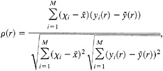
where M is the total number of meshes, χ̄ is the mean of χi, and ӯ(r) is the mean of yi(r). ρ(r) is calculated for coda Q−1 at four different frequencies (1.5, 3, 6, and 12 Hz) and three different lapse time windows—namely, 15–30, 20–45, and 30–60 sec measured from the origin time. As shown in Figs. 1–3, the autocorrelation functions are similar among different frequencies but clearly depend on the selected time window. The longer and later time window gives the slower decay in the autocorrelation with the distance separation. If we define the distance at which the correlation first comes close to 0 as the coherence distance, the average coherence distance is ≈135 km for the time window 30–60 sec, 90 km for the window 20–45 sec, and 45 km for the window 15–30 sec.
The above observation offers strong support to the assumption that coda waves are composed of S to S back-scattering waves, because the distances traveled by S waves with a typical crustal S wave velocity of 3.5 km/sec in half the lapse time 60, 45, and 30 sec are, respectively, 105, 79, and 53 km, which are close to the corresponding coherence distance—namely, 135, 90, and 45 km. In other words, the coda Q−1 measured from a time window represents the seismic attenuation property of the earth’s crust averaged over the volume traversed by the singly back-scattering S waves.
Ouyang and Aki (45) constructed maps of coda Q−1 for various frequencies and time windows using the enormous digital data from the Southern California Seismic Network, now available at the Southern California Earthquake Center data center.
To construct a map of coda Q−1, I first assign each coda Q−1 measurement at the midpoint between the station and the
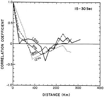
FIG. 1. Spatial autocorrelation function of coda Q−1 at various frequencies measured from the time window 15–30 sec in southern California obtained by Peng (44).
earthquake epicenter. I then average coda Q−1 measurements for midpoints lying within a 0.2°×0.2° region and plot the average value at the center of this region. Fig. 4 shows an example of such a map for the center frequency 12 Hz and the coda window 20–30 sec from the origin time. The values of the averages are represented by different sizes of dots, with larger dots for larger coda Q−1, corresponding to averaged coda Q−1 (10−3) within a range as indicated on the right. Coda Q−1 measurements made from 8931 seismograms were used to construct the map shown in Fig. 4. These seismograms are from 2446 earthquakes recorded at 161 seismic stations. The hypocentral distances are shorter than 35 km in order to meet the condition that the coda window starts at the lapse time later than twice the S wave arrival time. The time window of 20–30 sec corresponds to the sampling region of radius 30–45 km.
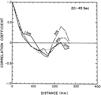
FIG. 2. Spatial autocorrelation function of coda Q−1 at various frequencies measured from the time window 20–45 sec in southern California obtained by Peng (44).
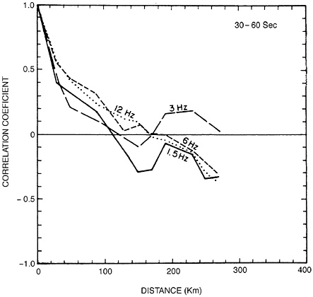
FIG. 3. Spatial autocorrelation function of coda Q−1 at various frequencies measured from the time window 30–60 sec in southern California obtained by Peng (44).
The map shows that the regional average of coda Q−1 for 12 Hz is 1.4×10⁻³. The geographic variation is rather small; 50% of the sites are within the range 1.2−1.5×10⁻³. There is a systematically low Q−1 value along the peninsular range, sandwiched between NW-SE trending high Q−1 zones. This pattern is remarkably similar to the map of P velocity at a depth of 20 km obtained by Hu et al. (46) by polarization inversion, and high velocity corresponds to high Q (low Q−1), and low velocity corresponds to low Q. The peninsular range also shows high isostatic anomaly, indicating high density according to Griscom and Jachens (47). The above correlation suggests that the coda Q−1 may reflect the material properties in the lower crust.
Temporal Change in Coda Q
Chouet (48) was the first to observe a significant temporal change in coda Q at Stone Canyon, California, which could not be attributed to changes in instrument response or in the epicenter locations, focal depths, or magnitudes of earthquakes used for the measurement. The change was associated with neither the rainfall in the area nor the occurrence of any particular earthquake but showed a weak negative correlation with the temporal change in a seismicity parameter called b value (49). The b value is defined in the Gutenberg-Richter formula log N=a−bM, where N is the frequency of earthquakes with magnitude greater than M.
Numerous studies made since (see ref. 50 for a critical review of early works) revealed that the temporal correlation between coda Q−1 and seismicity is not as simple as the spatial correlation described in the preceding section.
In a number of cases (51–56), coda Q−1 shows a peak during a period of 1–3 years before the occurrence of a major earthquake. A similar precursory pattern showed up also before the 1989 Loma Prieta earthquake in central California and the Landers earthquake in southern California (57). From the study of coda Q−1 over a period of >50 years for both central and southern California, Jin and Aki (57) had to conclude that the coda Q−1 precursor is not reliable, because a similar pattern sometimes is not followed by a major earthquake, and some major earthquakes were not preceded by the pattern.
A rather surprisingly consistent observation made by these studies is that coda Q−1 tends to take a minimum value during the period of high aftershock activity (51, 52, 55) except for the recent Northridge earthquake (45). Furthermore, Tsukuda (58) found in the epicentral area of the 1983 Misasa earthquake that a period of high coda Q−1 from 1977 to 1980 corresponds to a low rate of seismicity (quiescence). These observations suggest that the temporal change in coda Q−1 may be related primarily to creep fractures in the ductile part of the lithosphere rather than in the shallower brittle part.
Several convincing cases were made also for the temporal correlation between coda Q−1 and b value. The result was at first puzzling because the correlation was negative in some cases (49, 53, 59) and positive in other cases (10, 58). To resolve this puzzle, Jin and Aki (10) proposed the creep model, in which creep fractures near the brittle-ductile transition zone of the lithosphere are assumed to have a characteristic size in a given seismic region. The increased creep activity in the ductile part would then increase the seismic attenuation and at the same time produce stress concentration in the upper brittle part favoring the occurrence of earthquakes with magnitude Mc corresponding to the characteristic size of the creep fracture. Then, if Mc is in the lower end of the magnitude range from which the b value is evaluated, the b value would show a positive correlation with coda Q−1, and if Mc is in the upper end the correlation would be negative.
The creep model is consistent with the observed behaviors of coda Q−1 during the periods of aftershocks and quiescence mentioned earlier. Another support for the deeper source of the coda Q−1 change comes from the observed coincidence
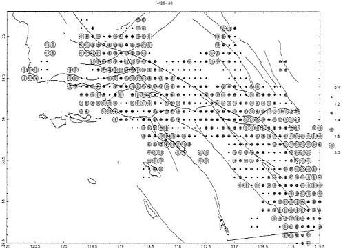
FIG. 4. The average coda Q−1 for midpoints (of the epicenter and the receiver) lying within a 0.2°×0.2° region for frequency 12 Hz and time window 20–30 sec. Larger circles correspond to greater coda Q−1 as indicated on the right (in 10−3).
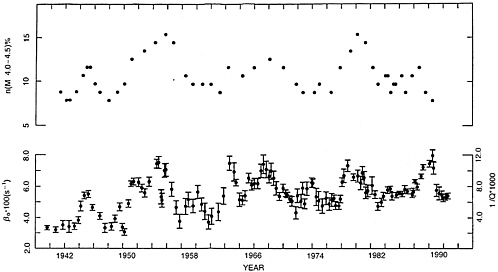
FIG. 5. Comparison between temporal variations of πfQc−1 (f is ≈2 Hz) and fractional frequency of earthquakes with magnitude 4.0<M< 4.5, for central California from Jin and Aki (11).
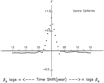
FIG. 6. Cross-correlation function between the two time series shown in Fig. 5.
between a large increase in coda Q−1 in southern California during 1986 and 1987 (10, 44) and the increase in electrical conductivity in the same region (60), which is attributed to the lower crust.
If the creep model is correct, the strongest correlation should be found between coda Q−1 and the rate of occurrence of earthquakes with Mc, and the correlation should always be positive. Indeed, Jin and Aki (11) found a remarkable positive correlation between coda Q−1 and the fraction of earthquakes in the magnitude range Mc< M < Mc+0.5 for both central and southern California. Fig. 5 shows the result for central California where the appropriate choice of Mc is 4.0. The correlation is highest (0.84) for the zero time lag and decays symmetrically with the time shift as shown in Fig. 6. A very similar result is obtained for southern California where the appropriate choice of Mc is 3.0. The correlation is again the highest (0.81) at the zero time lag.
Thus, my current working hypothesis is that the temporal change in coda Q−1 reflects the activity of creep fractures in the ductile part of the lithosphere. The ductile part of the lithosphere is larger than the brittle part. The deformation in the ductile part is the source of stress in the brittle part. Although it was found that the coda Q−1 precursor is not reliable, the study of spatial and temporal variation in coda Q−1 may still be promising for understanding the loading process that leads to earthquakes in the brittle part.
Discussion
The characteristic magnitude Mc attributed to the characteristic scale length of creep fracture in southern California is 3.0, which corresponds to the fault length of a few hundred meters. The closeness of this length to the fault zone width estimated from trapped modes suggests a generic relation between them.
Our creep model may be relevant for understanding some of the intriguing precursory phenomena. For example, the decrease in b value coincident with the increase in coda Q−1 before the Tangshan earthquake of 1976 (53) may be attributed to the activated creep fracture in the ductile crust with scale length corresponding to a Mc value of 4–5, which increased the stress in the brittle part of the crust.
As mentioned earlier, the overall self-similarity governing earthquakes with source dimension from 10 cm to 100 km requires a discrete hierarchy of characteristic scale lengths. Recently, Sornette and Sammis (61) reported a logarithmic periodicity in the precursory seismicity before the Loma Prieta earthquake of 1989. The Renormalization Group equation which leads to the logarithmic periodicity is discrete. One jumps from one time to another by a finite amount, implying the existence of a discrete hierarchy of characteristic scales. We may be at a threshold of building a truly physical theory of earthquake prediction based on the well-defined structure of the seismogenic zone.
This work was supported by the Southern California Earthquake Center under National Science Foundation Cooperative Agreement EAR-8920136 and U.S. Geological Survey Cooperative Agreement –14–08–0001–A0899 and in part by Department of Energy Grant DE-FG03–87ER13807.
1. Abercrombie, R.E. & Leary, P.C. (1993) Geophys. Res. Lett. 20, 1511–1514.
2. Aki, K. (1967) J. Geophys. Res. 72, 1217–1232.
3. Berckhemer, H. (1962) Gerlands. Beitr. Geophys. 72, 5–26.
4. Chouet, B., Aki, K. & Tsujiura, M. (1978) Bull. Seismol. Soc. Am. 68, 49–79.
5. Rautian, T.G., Khalturin, V. I., Martinov, V.G. & Molnar, P. (1978) Bull Seismol. Soc. Am. 68, 749–792.
6. Papageorgiou, A.S. & Aki, K. (1983) Bull Seismol. Soc. Am. 73, 953–978.
7. Hanks, T.C. (1982) Bull Seismol. Soc. Am. 72, 1867–1880.
8. Okubo, P.G. & Aki, K. (1987) J. Geophys. Res. 92, 345–355.
9. Aki, K. (1987) J. Geophys. Res. 92, 1349–1355.
10. Jin, A. & Aki, K. (1989) J. Geophys. Res. 94, 14041–14059.
11. Jin, A. & Aki, K. (1993) J. Geodyn. 17, 95–120.
12. Li, Y.G., Aki, K., Adams, D., Hasemi, A. & Lee, W.H.K. (1994) J. Geophys. Res. 99, 11705–11722.
13. Leary, P.C., Li, Y.-G. & Aki, K. (1987) Geophys. J.R.Astron. Soc. 91, 461–484.
14. Li, Y.-G. & Leary, P.C. (1990) Bull. Seismol. Soc. Am. 80, 1245–1271.
15. Li, Y.-G., Leary, P.C., Aki, K. & Malin, P.E. (1990) Science 249, 763–766.
16. Johnson, A.M., Fleming, R.W. & Cruikshank, K.M. (1994) Bull Seismol. Soc. Am. 84, 499–510.
17. Li, Y., Aki, K., Chin, B.-H., Adams, D., Beltas, P. & Chen, J. (1995) Seismol. Res. Lett. 66, 39.
18. Li, Y.-G., Henyey, T.L. & Leary, P.C. (1992) J. Geophys. Res. 97, 8817–8830.
19. Mooney, W.D. & Meissner, R. (1992) in Continental Lower Crust, eds. Fountan, D.M., Arculus, R. & Kay, R.W. (Elsevier, Amsterdam), pp. 45–79.
20. Sabine, W.C. (1922) Collected Papers on Acoustics (Harvard Univ. Press, Cambridge, MA).
21. Aki, K. (1969) J. Geophys. Res. 74, 615–631.
22. Rautian, T.G. & Khalturin, V. I. (1978) Bull. Seismol. Soc. Am. 68, 923–948.
23. Herraiz, M. & Espinosa, A.F. (1987) PAGEOPH 125, 499–577.
24. Su, F., Aki, K. & Biswas, N.N. (1991) Bull. Seismol. Soc. Am. 81, 162–178.
25. Su, F., Aki, K., Teng, T., Zeng, Y., Koyanagi, S. & Mayeda, K. (1992) Bull Seismol. Soc. Am. 82, 580–602.
26. Aki, K. (1980) Phys. Earth Planet. Inter. 21, 50–60.
27. Mayeda, K., Koyanagi, S., Hoshiba, M., Aki, K. & Zeng, Y. (1992) J. Geophys. Res. 97, 6643–6659.
28. Aki, K. & Chouet, B. (1975) J. Geophys. Res. 80, 3322–3342.
29. Tsujiura, M. (1978) Bull. Earthquake Res. Inst. 53, 1–48.
30. Aki, K. (1992) Bull Seismol. Soc. Am. 82, 1969–1972.
31. Zeng, Y. (1993) Bull. Seismol. Soc. Am. 83, 1264–1277.
32. Aki, K. (1981) in Identification of Seismic Sources—Earthquake or Underground Explosion, eds. Husebye, E.S. & Mykkeltveit, S. (Reidel, Dordrecht, The Netherlands), pp. 515–541.
33. Frankel, A. & Clayton, R.W. (1986) J. Geophys. Res. 91, 6465– 6489.
34. Matsunami, K. (1991) Phys. Earth Planet. Inter. 67, 104–114.
35. Shang, T. & Gao, L.S. (1988) Sci. Sin. Ser. V 31, 1503–1514.
36. Aki, K. (1991) Phys. Earth Planet. Inter. 67, 1–3.
37. Wu, R. (1985) Geophys. J.R.Astron. Soc. 82, 57–80.
38. Gao, L.S., Lee, L.C., Biswas, N.N. & Aki, K. (1983) Bull. Seismol. Soc. Am. 73, 377–390.
39. Zeng, Y., Su, F. & Aki, K. (1991) J. Geophys. Res. 96, 607–619.
40. Hoshiba, M, Sato, H. & Fehler, M. (1991) Paper Meteorol. Geophys. 42, 65–91.
41. Hoshiba, M. (1993) J. Geophys. Res. 98, 15809–15824.
42. Jin, A., Mayeda, K., Adams, D. & Aki, K. (1994) J. Geophys. Res. 99, 17835–17848.
43. Singh, S.K. & Herrmann, R.B. (1983) J. Geophys. Res. 88, 527–538.
44. Peng, J.Y. (1989) Thesis (Univ. Southern California, Los Angeles).
45. Ouyang, H. & Aki, K. (1994) Eos 75, 168 (abstr.).
46. Hu, G., Menke, W. & Powell, C. (1994) J. Geophys. Res. 99, 15245–15256.
47. Griscom, A. & Jachens, R.C. (1990) San Andreas Fault System, California (U.S. Geological Survey, Reston, Va), Professional Paper 1515, pp. 239–260.
48. Chouet, B. (1979) Geophys. Res. Lett. 6, 143–146.
49. Aki, K. (1985) Earthquake Prediction Res. 3, 219–230.
50. Sato, H. (1988) PAGEOPH 126, 465–498.
51. Gusev, A.A. & Lemzikov, V.K. (1984) Vulk. Seismol. 4, 76–90.
52. Novelo-Casanova, D. A, Berg, E., Hsu, H. & Helsley, C.E. (1985) Geophys. Res. Lett. 12, 789–792.
53. Jin, A. & Aki, K. (1986) J. Geophys. Res. 91, 665–673.
54. Sato, H. (1986) J. Geophys. Res. 91, 2049–2061.
55. Faulkner, J. (1988) Thesis (Univ. of Southern California, Los Angeles).
56. Su, F. & Aki, K. (1990) PAGEOPH 133, 23–52.
57. Jin, A. & Aki, K. (1993) J. Geodyn. 17, 95–120.
58. Tsukuda, T. (1988) PAGEOPH 128, 261–280.
59. Robinson, R. (1987) PAGEOPH 125, 579–596.
60. Madden, T.R., LaTorraca, G.A. & Park, S.K. (1993) J. Geophys. Res. 98, 795–808.
61. Sornette, D. & Sammis, C.G. (1995) J. Phys. (Paris), in press.


