(NAS Colloquium) Earthquake Prediction: The Scientific Challenge (1996)

This paper was presented at a colloquium entitled “Earthquake Prediction: The Scientific Challenge,” organized by Lean Knopoff (Chair), Keiiti Aki, Clarence R.Allen, James R.Rice, and Lynn R.Sykes, held February 10 and 11, 1995, at the National Academy of Sciences in Irvine, CA.

(premonitory seismicity patterns/dynamics of seismicity/chaotic systems/instability)

V.I.KEILIS-BOROK

International Institute of Earthquake Prediction Theory and Mathematical Geophysics, Russian Academy of Sciences, Warshavskoye shosse 79, kor 2, Moscow 113556, Russia

ABSTRACT An earthquake of magnitude M and linear source dimension L(M) is preceded within a few years by certain patterns of seismicity in the magnitude range down to about (M−3) in an area of linear dimension about 5L−10L. Prediction algorithms based on such patterns may allow one to predict ≈80% of strong earthquakes with alarms occupying altogether 20–30% of the time-space considered. An area of alarm can be narrowed down to 2L-3L when observations include lower magnitudes, down to about (M−4). In spite of their limited accuracy, such predictions open a possibility to prevent considerable damage. The following findings may provide for further development of prediction methods: (i) long-range correlations in fault system dynamics and accordingly large size of the areas over which different observed fields could be averaged and analyzed jointly, (ii) specific symptoms of an approaching strong earthquake, (iii) the partial similarity of these symptoms worldwide, (iv) the fact that some of them are not Earth specific: we probably encountered in seismicity the symptoms of instability common for a wide class of nonlinear systems.

Commonly known are five major stages of earthquake prediction, which are usually distinguished. They differ in characteristic time intervals for which an alarm is declared. The background stage provides a map of maximal possible magnitudes and a map of average recurrence time for strong earthquakes of different magnitudes. The other four stages are as follows: long-term (tens of years), intermediate-term (years), short-term (months to weeks), and immediate (days and less). A smaller time interval in present predictions does not necessarily mean a smaller area of alarm where a strong earthquake has to be expected. Possibility of prediction has been explored separately for different stages and, with rare exceptions, their connection is not yet achieved. Here we review the intermediate-term stage.

A new understanding of the earthquake prediction problem and the whole dynamics of seismicity has crystallized over the past decade: the seismically active lithosphere has become regarded as a hierarchical nonlinear (chaotic) dissipative system (e.g., see refs. 1–3). The simplest source of nonlinearity of this system is abrupt triggering of an earthquake when the stress exceeds the strength of a fault. Other powerful sources of nonlinearity are provided by a multitude of the processes controlling the distribution of strength within the lithosphere. Among such processes are nonlinear filtration of fluids (4), stress corrosion, caused by surface-active fluids (5, 6), dissolution of rocks (6), buckling, microfracturing, phase transformation of the minerals, etc. Except for rather special cases, none of these mechanisms predominates to such an extent that the others can be neglected. In the time scale relevant to intermediate-term earthquake prediction, these mechanisms seem to make the lithosphere a chaotic system; this is an inevitable conjecture, but it is not yet proven in a mathematical sense.

Predictability of a chaotic process may be achieved in two ways. First, such process often follows a certain scenario; recognizing its beginning one would know the subsequent development. Second, a chaotic process may become predictable, up to a limit, after an averaging. Most of the results described below are obtained in the second way. It was found that the approach of a “strong” earthquake may be indicated by certain patterns in an earthquake sequence; they are called premonitory seismicity patterns and are used in prediction algorithms reviewed here.

A test of prediction algorithms is crucially important, since they are inevitably adjusted retrospectively. The algorithms discussed here were tested first by applying them to the regions or time periods not involved either in the design of the algorithm or in the fitting of adjustable parameters. The ultimate test is the advance prediction. We review here only such prediction methods that are formally defined so that their performance can be tested and statistical significance can be evaluated. A methodology for such evaluation is suggested (7).

The search of premonitory seismicity patterns in observed and in computer-simulated seismicity revealed four of their basic features, which are important for understanding the earthquake prediction problem. In hindsight, they are obvious, being common for many nonlinear systems. For seismology, they are hardly news either, as they correspond to many well-known traits of the dynamics of seismicity, such as the Gutenberg-Richter relation, the Omori law, and migration of seismicity (8). Nevertheless, these features are the new paradigms in earthquake prediction research where they are often overlooked. We outline them here as a background for the discussion of prediction algorithms in the next section.

(i) Long-Range Correlations. The generation of an earthquake is not localized around its source. A flow of earthquakes is generated by a system of blocks and faults rather than each earthquake by a single fault. Accordingly, the signal of an approaching earthquake may inconveniently come not from a narrow vicinity of the incipient source but from a much wider area; its linear dimension at intermediate-term stage is at least 5L(M)−10L(M), with M being the magnitude of the incipient earthquake and L(M) the characteristic length of its source. Moreover, according to ref. 9, this dimension can reach

≈100L: the Parkfield earthquakes with a magnitude of ≈6 are preceded by a rise of activity in as far as the Great Basin or the Gulf of California. Such an area may include different types of faults. Many examples for different regions worldwide can be found (10–13). Other evidence and possible mechanisms of long-range correlations are discussed in the last section.

(ii) Premonitory Phenomena. Before a strong earthquake, the earthquake flow in a medium magnitude range becomes more intense and irregular; earthquakes become more clustered in space and time and the range of their correlation probably increases (12, 13). These symptoms may be interpreted as an increased response of the lithosphere to excitation (possibly provided by consecutive earthquakes themselves); such a response is symptomatic of a critical state in many other nonlinear systems. Some of these symptoms are formally defined in the next section.

(iii) Similarity. In robust definition, the normalized premonitory phenomena are identical in the magnitude range of at least M≥4.5 and for a wide variety of neotectonic environments (12–14), which include subduction zones, transform faults, intraplate faults in the platforms, induced seismicity near artificial lakes, and rock bursts in mines. This similarity is limited and on its background the regional variations of premonitory phenomena begin to emerge.

(iv) The Non-Earth-Specific Nature of Some Premonitory Phenomena. Many premonitory seismicity patterns are found in the models of exceedingly simple design. Some of such models, consisting of lattices of interacting point elements, are totally free of Earth-specific (or even solid-body-specific) mechanisms (15–17); other models retain only the simplest mechanism-friction (18–21). A stochastic model suggested in ref. 22 goes a long way toward explaining swarms, quiescence, foreshocks, and mainshocks as a coordinated sequence.

The algorithms reviewed here are based on a common general scheme of data analysis and on premonitory seismicity patterns with similar scaling and normalization. We outline these common features first.

Scheme of Data Analysis. The scheme of data analysis (Fig. 1) can be summarized as follows:

1. Strong earthquakes are identified by the condition M≥ M₀. M₀ is the given threshold chosen in such a way that the average time interval between strong earthquakes is suffi

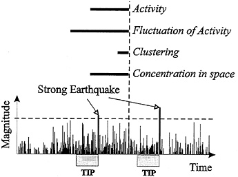
FIG. 1. General scheme of prediction. Vertical lines show earthquake sequence in an area. Several traits of this sequence are defined in sliding time windows shown by horizontal bars. TIPs (alarms) are recognized by one or several such traits.

2. ciently large in the area considered. The intervals (M₀, M₀+ 0.5) may be analyzed separately.

3. Prediction is aimed at determination of a time of increased probability (TIP) that is the time interval within which a strong earthquake has to be expected.

4. A seismic region under investigation is overlaid by areas whose size depends on M₀. In each area, the sequence of earthquakes is analyzed. We determine its robust averaged traits, which are useful for prediction (the most commonly considered traits are indicated in Fig. 1). These traits are depicted by functions of time t defined in the sliding time windows with a common end t. We search for the functions whose values have different distributions inside and outside the TIPs. One or several of such functions could be used for prediction; a combination of precursors may be useful for prediction even if some of them show unsatisfactory performance when used separately. A variety of premonitory seismicity patterns was found in such a way.

Obviously this scheme is open for inclusion of other traits and other data, not necessarily seismological ones.

Major Common Characteristics. Major common characteristics of premonitory patterns considered here include the following:

1. Robustness. We have to look for the patterns common in a wide variety of regions and magnitude ranges as well as within sufficiently long time periods; otherwise the test of prediction algorithms would be practically impossible. Accordingly, premonitory patterns are given robust definitions in which the diversity of circumstances is averaged away while some predictive power is retained.

2. Time scale. The earthquake flow is averaged over time intervals a few years long and duration of alarms is about the same. These intervals do not depend on M₀, while according to the Gutenberg-Richter relation the earthquakes with smaller magnitudes occur more frequently; the average time between the earthquakes of magnitude M is proportional to 10^BM.* This is not a contradiction, since the Gutenberg-Richter law refers to a given region, the same for all magnitudes, while premonitory patterns are defined for an area with a linear dimension proportional to 10^aM0. The average time between the earthquakes in such an area would be proportional to 10(B−av)M₀ where v is the fractal dimension of the cloud of the epicenters. The existing estimations of parameters B (≈1), a (0.5−1), and v (1.2−2) do not contradict the hypothesis that the expression in brackets is close to 0 as if the earthquakes with different magnitudes have about the same recurrence time in their own cells. Still, for some premonitory patterns the time scale may depend on M₀ (23).

3. Normalization. Normalization of an earthquake flow is necessary to ensure that a prediction algorithm can be applied with the same set of adjustable parameters in the regions with different seismicity. In the studies reviewed here, an earthquake flow is normalized by the minimal magnitude cutoff M_min? defined by one of the two conditions: M_min=(M₀−a) or Ñ(M_min)=b, Ñ being the average annual number of earthquakes with magnitude M≥M_min; parameters a and b are common for all areas. If the second condition is applied, the intensity of the earthquake flow considered is the same in different areas, while M_min may be different.

I now describe the prediction algorithms; the first one is defined in greater detail, for illustration.

Algorithm M8 (13) was designed by retrospective analysis of seismicity preceding the greatest (M≥8) earthquakes world-

wide, hence its name. The scheme of prediction described above (Fig. 1) is implemented by this algorithm in the following way:

1. The territory considered is scanned by overlapping circles with the diameter D(M₀). A set of such circles, considered for prediction of Californian earthquakes with M≥7, is shown in Fig. 2A.

2. Within each circle, the sequence of earthquakes is considered with aftershocks eliminated {t_i, m_i, h_i, b_i(e)}, i=1, 2… Here t_i is the origin time, t_i≤t_i+1; m is the magnitude, h_i is focal depth, and b(e_i) is the number of aftershocks during the first e days. The sequence is normalized by lower magnitude cutoff M_min(Ñ), with a standard value of Ñ.

3. Several functions of time t characterizing this sequence are computed in the sliding time windows (t−s, t) and magnitude range M₀>M_i≥M_min(Ñ). These functions include

1. N(t), the number of the main shocks.

2. L(t), the deviation of N(t) from the long-term trend.

   

   N_cum(t) is the total number of the main shocks with M≥M_min from the beginning of the sequence t₀ to t.

3. Z(t), concentration of the main shocks estimated as the ratio of the average diameter of the source l to the average distance between them r. The following coarse estimations of r and l are assumed: r~N^−1/3, l~N⁻¹·Σ(t), where Σ(t)= Σ_i 10^d(Mi−f), and M_min≤M_i≤M₀−g; the value of d is chosen in such a way that each summand is proportional to the linear dimension of the source (in practice, to the cubic root of energy, E^1/3). A more refined estimation of Z has been considered in ref. 24.

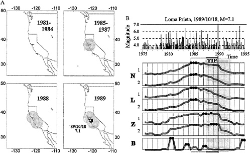
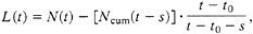
FIG. 2. Advance prediction by algorithm M8 of the Loma Prieta, California, earthquake, 1989, M=7.1. (A) Areas of alarms. The territory was scanned by eight overlapping circles. TIPs were diagnosed in the darkened circles. Star shows the epicenter of the Loma Prieta earthquake. Solid polygon shows the reduced area of alarm; it is determined in retrospection by applying algorithm Mendocino Scenario described below. (B) Diagnosis of the TIP in the third from she bottom circle. Very large values of functions (dots) are concentrated in a 3-year interval, 1985–1987 (light rectangle). TIP was declared for the next 5 years (darker rectangle). Other explanations are given in the text.

4. B(t)=max_{i}{b_i}, the maximal number of aftershocks (a measure of earthquake clustering); the earthquake sequence {i} is considered in the time window (t−s′, t) and in the magnitude range (M₀−p, M₀−q).

5. Each of the functions N, L, Z is calculated for Ñ=20 and Ñ=10. As a result, the earthquake sequence is given a robust averaged description by seven functions: N, L, Z (twice each) and B.

6. Very large values are identified for each function using the condition that they exceed Q percentiles (i.e., they are higher than Q% of the encountered values).

7. An alarm or TIP is declared for 5 years, when at least 6 of 7 functions, including B, become very large within a narrow time window (t−u, t). To make a prediction more stable, this condition is required for two consecutive moments, t and t+0.5 years.

Standard Parameters. The following standard values of parameters indicated above are fixed in the algorithm M8^‡: D(M₀)={exp(M₀−5.6)+1}° in degrees of meridian (this is 276, 560, and 1333 km for M₀=6, 7, and 8, respectively), s=6 years, s′=1 year, g=0.5, p=2, q=0.2, u=3 years, Q=75% for B and 90% for the other 6 functions.

Obviously, the magnitude scale used in this and other algorithms described here should not saturate within the magnitude range considered; otherwise computation of the function becomes meaningless. Accordingly, maximal magnitudes indicated in the catalog are used; MS usually is taken for larger magnitudes and mb for smaller ones. The use of only the mb scale, which saturates at about mb=6, renders invalid the “test of algorithm M8” in ref. 25.

An example of prediction by algorithm M8 is given in Fig. 2 . Shown at the top of Fig. 2B is the sequence of the main shocks in the third from the bottom circle in Fig. 2A. Seven functions describing the earthquake flow are plotted below; indexes 1 and 2 correspond to Ñ=10 and 20, respectively. Very large values are indicated by the solid circles. The start of the TIP (July 1987) is indicated by a vertical line. Loma Prieta earthquake, California, 1989, M=7.1, occurred 28 months later. Note that in the adjacent circle the TIP started in 1985. A more detailed case history of this prediction (made in advance) is described in ref. 26.

Performance. Algorithm M8 was first applied retrospectively (13) with prefixed parameters to the following 12 regions not considered in its development (the values of M₀, defining a strong earthquake, are indicated in brackets).

Circum Pacific belt. Central America [8], Kamchatka-Kuril Island [7.5], Japan-Taiwan [7.5], South America [7.5], and Western US [7.5 and 7].

Alpine-Himalayan belt. The Lake Baikal and the Stanovoy range [6.7], the Caucasus [6.5], the Pamir and Tien Shan [6.5], Eastern Tien Shan [6.5], Western Turkmenia [6.5], the Apennines [6.5], and the area of induced seismicity near Koyna reservoir [4.9].

The time intervals from 9 to 40 years long, all ending around 1985, were considered in different regions, depending on availability of data.

An experiment in advance prediction (27, 28) started in about 1985 for the Circum Pacific belt [8 and 7.5], western United States [7.0], the seven above-mentioned regions of the Alpine-Himalayan belt, and Lesser Antilles [6]. The breakdown of predictions may be summarized in Table 1.

Algorithm CN (12, 29) was designed by retrospective analysis of seismicity patterns preceding the earthquakes with M≥6.5 in California and the adjacent part of Nevada, hence its name. The essence of this algorithm can be summarized as follows.

1. Areas of investigation are selected taking into account the spatial distribution of seismicity.

2. Within each area we consider the earthquakes with the average annual number Ñ=3 (after elimination of aftershocks). As compared with Ñ=20 in algorithm M8 this gives a higher magnitude cutoff M_min.

3. The sequence of earthquakes is described by 9 functions. Three of them—N, Z, and B—are similar to the ones defined above, although with different values of the numerical parameters. Other functions depict the share of relatively higher magnitudes in the sequence considered, the different variations of this sequence in time, and the average value of source areas, where the slip (or rupture) took place.

4. Following the pattern recognition routine (30), these functions are coarsely discretized so that we distinguish only large, medium, and small values divided by 2/3 and 1/3 percentiles or large and small values divided by 1/2 percentile.

5. The alarms (TIPs) are determined by certain combinations—pairs or triplets—of these discretized functions; these combinations were found by applying the pattern recognition algorithm called subclasses (30). Qualitatively, a TIP is diagnosed when earthquake clustering is high, seismicity is irregular, high and growing, and the increase of seismicity was

6. preceded by a quiescence. Examples of prediction by algorithm CN are given in Fig. 3.

Performance. Algorithm CN was first tested retrospectively with prefixed parameters for the following 21 regions (12).

Circum Pacific belt. Northern and Southern California [6.4], the Gulf of California [6.6], Cocos plate margins [6.5], and adjacent to the belt Lesser Antillean arc [5.5].

Alpine-Himalayan belt. The area of intermediate-depth earthquakes in Vrancea, East Carpatheans [6.4], the Pamir [6.5], the Tien Shan [6.5], the Baikal [6.4], Central Italy [5.6], the Caucasus [6.4], Kangra, Nepal and Assam regions in the Himalayas [6.4], Krasnovodsk, Elburz and Kopet Dag areas [6.4], and the Dead Sea rift [5.0].

Low seismicity regions. Northern and Southern Appalachians [5.0], Brabant-Ardennes [4.5].

The earthquake catalogs available allowed one to consider time intervals from 12 to 22 years in each region, except 32 years in Italy and 45 years in California. Sixty strong earthquakes occurred in all the regions during these intervals. Of them 50 (83%) occurred during the TIPs and 10 were missed. TIPs in a region occupy on an average 27% of the time, from 2 to 4 years per earthquake (except 6–8 years in the southern part of Dead Sea rift, Kopet Dag, and Vrancea).

An experiment in advance prediction for all these regions was subsequently carried out for 3–12 more years in a region (31). The breakdown of predictions is as follows:

strong earthquakes M₀≤M≤M₀+0.5 M>M₀+0.5

total/predicted 11/8(73%) 11/4(36%)

The duration of a TIP was from 1 to 2 years per earthquake but 6 years in Nepal. We see that prediction by algorithm CN is more reliable for strong earthquakes, which occur on an average once in 7–10 years (Ñ=0.15−0.1); prediction of stronger earthquakes should probably be made separately, in larger areas. This breakdown is not made for the retrospective test, since the magnitudes were often rounded up to 0.5 during the corresponding time intervals.

On the whole, algorithm CN gets 2/3 of strong earthquakes within the TIPs, occupying 1/3 of the time. In subduction zones, performance of this algorithm is poor, although the 9 functions, mentioned above, do have different distributions within and outside of the TIPs. It seems that other combinations of functions have to be used for subduction zones.

Algorithm Mendocino scenario (32) is designed to solve the following problem: given a TIP diagnosed for certain territory U at the moment T, we have to find within U a smaller area V where the predicted strong earthquake has to be expected. To apply this algorithm, we need a reasonably complete catalog of

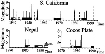
FIG. 3. Strong earthquakes and TIPs diagnosed by algorithm CN (12). Vertical lines show moments of strong earthquakes, dashed lines indicate failures to predict. Solid, hatched, and open bars show correct, false, and current TIPs.

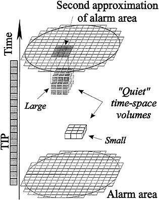
FIG. 4. Reduction of alarm area by applying the Mendocino scenario algorithm (32). Explanations are given in the text.

earthquakes with magnitudes M ≥ (M₀–4), which is a much lower threshold than in algorithms M8 and CN. This algorithm was designed by retrospective analysis of seismicity prior to the Eureka earthquake (1980; M=7.2) near Cape Mendocino in California, hence its name. Its essence can be summarized as follows (Fig. 4).

(i) Territory U is scanned by small squares of s×s size. Let (i, j) be the discretized coordinates of the centers of the squares.

(ii) Within each square (i, j) the number of earthquakes n(i,j,k), aftershocks included, is calculated for consecutive short time windows u months long starting from the time t₀= (T—6 years) onward, to allow for the earthquakes that contributed to the TIP’s diagnosis; k is the sequence number of a time window. In this way the time-space considered is divided into small boxes (i, j, k) of the size (s×s×u).

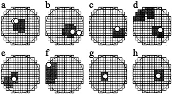
FIG. 5. Applications of Mendocino scenario algorithm (28). Circles and dark polygons show alarm areas obtained respectively by M8 and Mendocino scenario algorithms. Small open circles show actual epicenters of strong earthquakes. In each case M₀=7.5 and the diameter D(M₀) of the circle is 853 km. Strong earthquakes: (a) Santa Cruz Island, 11/28/1985 and 12/21/1985, M=7.6. (b) New Guinea, 02/08/1987, M=7.6 and 10/16/1987, M=7.7. (c) Costa Rica, 04/22/1991, M=7.6. (d) Landers, California, 06/28/1992, M=7.6. (e) Guam Island, 08/08/1993, M=8.2. (f) Fiji, 03/09/1994, M=7.6. (g) Shikotan Island, 10/04/1994, M=8.3. (h) Tonga, 04/07/1995, M=8.0.

(iii) Quiet boxes are singled out for each square; they are defined by the condition that n(i, j, k) is below Q percentile.

(iv) The clusters of q or more quiet boxes connected in space or in time are identified. Area V is the territorial projection of these clusters, as illustrated in Fig. 4. The standard values of parameters adjusted for the case of the Eureka earthquake are as follows: u=2 months, Q=10%, q=4, and s=3D/16, D being the diameter of the circle used in algorithm M8.

A detailed description of the Mendocino Scenario has been given in ref. 32.

Performance. The Mendocino Scenario with prefixed parameters was first applied in retrospect (32) to 17 areas of the TIPs U: 12 areas in the Circum Pacific belt, 4 in the Tien Shan, and 1 in Armenia. Later on 16 more areas U with values of M₀ from 6 to 8 were analyzed (28); the results are illustrated in Fig. 5. The breakdown of predictions is given in Table 2.

The reduced areas of alarm V were 4–14 times smaller than the original areas U, 7 times on an average, but four epicenters were missed. In case when the area V is not found, the alarm continues for the whole area U. Sometimes an area V closely outlines the source of the subsequent strong earthquake (33), which may be the limit of accuracy for intermediate-term prediction.

Consider a strong earthquake with magnitude M₁ and occurrence time t₁. The problem is to predict whether the next strong earthquake with magnitude M₂≥(M₁−a) will occur before the time (t₁+T) within distance R(M₁) from the epicenter of the first earthquake; this may be a strong aftershock or the next strong main shock. To solve this problem, analyze the catalog of the aftershocks of the first earthquake during the first s days and the catalog of earthquakes during S years before it, both for magnitudes above M₁−m. The aftershocks are counted within the same distance R(M₁); the preceding earthquakes are counted within a larger distance CR.

The Algorithm. The algorithm for such predictions was found by a retrospective analysis of 21 Californian earthquakes with M≥6.4 (34). It can be briefly described as follows:

1. Seven characteristics of the sequence of the aftershocks are calculated, reflecting the number of the aftershocks, the total area of their sources, their maximal distance from the main shock, and the irregularity of this sequence. One more characteristic is the number of earthquakes in the time interval (t₁−S, t₁−S′) preceding the first strong earthquake. As in the algorithm CN, we distinguish only coarse values of each characteristic, large and small or large, medium and small.

2. Prediction is made in two steps.

1. If the number of the aftershocks is below a threshold D), the next strong earthquake is not expected within the above time and distance whatever other characteristics.

2. If this number is D or more, 8 characteristics listed above are considered. The algorithm of prediction was determined by using the pattern recognition algorithm called Hamming distance (38). Qualitatively, the occurrence of the next strong earthquake is predicted in the case when the number of the aftershocks is large, their sequence is highly irregular in time, they are concentrated closely to the epicenter of the main shock, and the activity preceding the first strong earthquake is low. A detailed description of this algorithm is given in ref. 34. The following standard values of numerical parameters were chosen: a=1, R(M₁)=0.03×10^0.5M1 km, C=1.5, T=1.5 years, m= 3, s=40 days, S=5 years, S′=90 days, and D=10.

Performance. This algorithm was tested with prefixed parameters in the following 9 regions (the minimal considered values of M₁ are indicated in brackets): California [6.4], the Balkans [7.0], the Pamir and Tien Shan [6.4], the Caucasus [6.4], Iberia and Maghrib [6.0], Italy [6.0], the Baikal and the Stanovoy range [5.5], Turkmenia [5.5], and the Dead Sea rift [5.0]. The breakdown of predictions is given in Table 3.

The rate of failures to predict (wrong No) is particularly low. Two current alarms have not expired yet.

One may note the case history of the prediction made after the Landers earthquake in California, 6/28/1992, M₁=7.6. It was predicted (36) that an earthquake with M ≥ 6.6 will occur at the distance up to R [7.6]=199 km within 1.5 years, so that the alarm expired on 12/28/93. The subsequent Northridge earthquake, M=6.6, occurred within this radius, but 19 days after the expiration of the alarm, so that the prediction was counted above as a false alarm. The applications of this algorithm in subduction zones are so far unsuccessful.

It is not clear yet whether some single premonitory pattern may compete in prediction with the algorithms described above. We shall enumerate here the patterns which are formally defined and therefore can be tested.

(i) Pattern Σ. Pattern Σ (23) is defined as the sum of the source areas in the earthquakes of medium magnitudes. This sum is coarsely estimated by the function Σ(t) with parameter d chosen in such a way that each summand is roughly proportional to E^2/3. An alarm is declared when this sum rises closely to the source area of a single earthquake of magnitude M₀. This is the first reported premonitory pattern featuring worldwide similarity and long-range correlations.

(ii) Burst of Aftershocks. Burst of aftershocks or pattern B (7, 39, 40) is defined as a main shock in a medium magnitude range with a large number of aftershocks, b_i≥C. So far this is the only premonitory seismicity pattern for which statistical significance in a strict sense is established (7).

(iii) Seismic Flux. Seismic flux is defined as a spatiotemporal distribution of seismicity smoothed by the magnitude-dependent Gaussian kernels (41). This smoothing is introduced to eliminate the coarse discretization of prediction algorithms in which an earthquake may be either counted in or not depending on a slight change of the hypocenter, or the magnitude, or the occurrence time. According to ref. 41, strong earthquakes are often preceded by a sharp extremum of seismic flux.

(iv) Other Formally Defined Premonitory Patterns. Other patterns include the swarms of the main shocks (42–44), the reversal of territorial distribution of seismicity that is activation of relatively quiet faults and quiescence on relatively active faults (45), the rise of seismic activity (10, 15, 23, 46), and the seismic quiescence (17, 47, 48). The last two patterns are not mutually exclusive, since they take place in different areas and time intervals. Less substantiated so far but sufficiently well defined are the following premonitory phenomena: increase of the range of spatial correlation in the earthquake flow (49), and log-periodic variations of the earthquake flow on the background of its exponential rise (16, 46, 50).

(v) Events Time Scale. Of particular promise is an analysis of precursors with time measured in the number of the earthquakes within a certain magnitude range (51). This time scale allows one to make a uniform analysis of foreshocks, main shocks, and aftershocks.

With exception of pattern B the rate of successes and errors for single patterns is yet little explored.

Performance of Prediction Algorithms. On average, the algorithms discussed above provide for the prediction of ≈80% of strong earthquakes in a given region with alarms occupying from 20% to 30% of space-time. This can be done on the basis of earthquake catalogs, routinely available in most of the regions. With more complete catalogs, the areas of alarm may be substantially reduced in the second approximation at the cost of additional failures to predict. So far, this performance was mainly evaluated in retrospective studies, although adjustable parameters were chosen a priori; preliminary results of decisive tests—by advance predictions—are encouraging.

There are serious limitations in this performance. The areas covered by alarms are large (in the first approximation) and the rate of false alarms is substantial. In the prediction of the next strong earthquake to come, its magnitude is estimated with low accuracy (≥M₁−1) and the first 10 or 40 days are not considered. Nevertheless, considerable damage may be prevented by such predictions, if their formulation is specific (though not necessarily precise) and if it includes the probability of a false alarm (e.g., see refs. 52 and 53).

Analysis of Model-Generated Seismicity. Analysis of model-generated seismicity confirms that the algorithms described above tap rather general symptoms of subcritical state. Algorithms CN and M8 were successfully applied to the earthquake sequences generated by a numerical two-dimensional block model (19) consisting of a brick wall of 20 blocks. All the functions characterizing an earthquake sequence in algorithm CN were successfully tested on a model consisting of interacting elastic discs.

At least two premonitory patterns depicting the raise of seismic activity have been found first in lattice-type models and after that in the observed seismicity. These patterns are the active zone size (21) and the upward bend of the Gutenberg-Richter relation for higher magnitudes (15). A similar premonitory change of this relation was found first in microfracturing of steel, with fracture size from 0.01 to 3 mm, and after that in seismicity, in the magnitude range from 3 to 6.5 (54).

Why Is a Stalemate in Earthquake Prediction Efforts Often Reported in Contradiction to the Studies Reviewed Here? In the author’s opinion, such a stalemate is due to the too biased search of possible precursors and it may be overcome if only there is an awareness that:

1. Non-local precursors are possible.

2. An averaging of observations is necessary: it is well known that a sure way not to predict a chaotic process is to consider it in a too fine detail.

3. Other stages of earthquake prediction besides background and immediate ones are important to prevent damage.

On Nonlocal Precursors. They are not the only manifestations of long-range correlations in the dynamics of seismicity. Other manifestations covering even larger distances include migration of seismicity along active faults up to the distances of 10³ km (8), correlation of the strongest earthquakes worldwide with perturbations of the Chandler wobble and Earth’s rotation (55), and alternate rises of seismicity in distant areas [such areas may be separated by hundreds of kilometers for

seismicity in magnitudes 5 range (9) and are even spread worldwide (56) for higher magnitudes].

Nevertheless, in earthquake prediction research long-range correlations are often regarded as counterintuitive, probably on the ground that in a wide class of simple elastic models redistribution of stress and strain after an earthquake would be confined to the vicinity of its source (Saint Venant principle). This argument is not applicable to a media with microinhomogenuities, including the lithosphere, where the loss of strength (damage) and the change of stress propagate not by entirely elastic mechanisms (e.g., see ref. 57). Moreover, redistribution of stress may be not relevant to this argument, since the earthquakes involved in long-range correlations may not trigger each other but reflect an underlying large-scale process such as microfluctuations in the movement of tectonic plates (9) or of crustal blocks within fault zones (18), migration of fluids (4), and perturbation of the ductile layer beneath the seismically active zone (58). Accordingly, there is no reason to look for premonitory phenomena only near an incipient fault break.

Unexplored Possibilities. Unexplored possibilities to develop the next generation of prediction algorithms seem to emerge, supported by the models reproducing the dynamics of seismicity (e.g., see refs. 2, 3, and 15–22), by abundance of relevant observations still not explored with adequate scaling and apart from that by a large collection of failures to predict, false alarms and successful predictions (e.g., see refs. 12, 13, 27, 28, 31, and 37). The algorithms described here may not use the most optimal sets of premonitory patterns and of the values of adjustable parameters, so that both sets can be possibly optimized. More fundamental possibilities can be enumerated as follows.

1. To consider premonitory phenomena separately inside and outside the potential nucleation zones of strong earthquakes. Such zones are formed around some fault junctions (30). Thus, as suggested in (59), some false alarms can be identified by high activity near these junctions.

2. To use for prediction the kinematic and geometric incompatibilities of the movements in a fault system (60, 61), reflecting its instability as a whole. In this way one may integrate the data on seismicity, creep, strain, GPS, and possibly on the migration of fluids.

3. To integrate different stages of prediction, following the singular experience of prediction of the Haicheng earthquake in China, 1976 (62).

While the performance of the algorithms described here is modest, only a small fraction of the wealth of unexplored possibilities has been made use of.

This paper was written when I was a visiting professor in the Department of the Earth, Atmospheric, and Planetary Sciences, Massachusetts Institute of Technology. I am very grateful to V. Kossobokov, I.Rotwain, M.Simons, F.Press, T.Jordan, A.Gabrielov, P.Molnar, Ch.Marone, and L.Knopoff for discussions, important suggestions, and highly relevant preprints. Ms. Z.Oparina provided patient and competent help in preparation of the manuscript. The studies reviewed in this paper were partly supported by the following grants: International Sciences Foundation (MB3000; MB3300), U.S. National Science Foundation (EAR 94 23818), International Association for the Promotion of Cooperation with Scientists from the Independent States of the Former Soviet Union (INTAS-93–809), Russian Foundation for Basic Research (944–05–16444a), and United States Geological Survey (under the Cooperation in Environment Protection, area IX).

1. Keilis-Borok, V.I. (1990) Rev. Geophys. 28, 19–34.

2. Turcotte, D.L. (1992) Fractals and Chaos in Geophysics (Cambridge Univ. Press, Cambridge, U.K.).

3. Newman, W.I., Gabrielov, A. & Turcotte, D.L., eds. (1994) Nonlinear Dynamics and Predictability of Geophysical Phenomena (Geophysical Monograph Series, IUGG-Am. Geophys. Union, Washington, DC).

4. Barenblatt, G.M., Keilis-Borok, V.I. & Monin, A.S. (1983) Dokl Akad. Nauk. SSSR 269, 831–834.

5. Gabrielov, A.M. & Keilis-Borok, V.I. (1983) PAGEOPH 121, 477–494.

6. Traskin, V.Yu. (1985) in Physical and Chemical Mechanics of Natural Dispersed Systems (Moscow Univ., Moscow), pp. 140– 196.

7. Molchan, G.M., Dmitrieva, O.E., Rotwain, I.M. & Dewey, J. (1990) Phys. Earth Planet. Inter. 61, 128–139.

8. Vilkovich, E.V. & Shnirman, M.G. (1982) Comput. Seismol 14, 27–37.

9. Press, F. & Allen, C. (1995) J. Geophys. Res. 100, 6421–6430.

10. Knopoff, L., Levshina, T., Keilis-Borok, V.I. & Mattoni, C. (1996) J. Geophys. Res. 101, 5779–5796.

11. Keilis-Borok, V. L (1982) Tectonophysics 85, 47–60.

12. Keilis-Borok, V.I. & Rotwain, I.M. (1990) Phys. Earth Planet. Inter. 61, 57–72.

13. Keilis-Borok, V.I. & Kossobokov, V.G. (1990) Phys. Earth Planet. Inter. 61, 73–83.

14. Kossobokov, V.G., Rastogi, B.K. & Gaur, V.K. (1989) Proc. Indian Acad. Set. Earth Planet. Sci. 98, No. 4, 309–318.

15. Narkunskaya, G.S. & Shnirman, M.G. (1994) Computational Seismology and Geodynamics (Am. Geophys. Union, Washington, DC), Vol. 1, pp. 20–24.

16. Newman, W.I., Turcotte, D.L. & Gabrielov, A. (1995) Phys. Rev. E 52, 4827–4835.

17. Ogata, Y. (1992) J. Geophys. Res. 97, 19845–19871.

18. Primakov, I.M., Rotwain, I.M. & Shnirman, M.G. (1993) Mathematical Modelling of Seismotectonic Processes in the Lithosphere for Earthquake Prediction Research (Nauka, Moscow), pp. 32–41.

19. Gabrielov, A.M., Levsina, T.A. & Rotwain, I.M. (1990) Phys. Earth Planet. Inter. 61, 18–28.

20. Shaw, B.E., Carlson, J.M. & Lander, J.S. (1992) J. Geophys. Res. 97, 479.

21. Kossobokov, V.G. & Carlson, J.M. (1995) J. Geophys. Res. 100, 6431–6441.

22. Yamashita, T. & Knopoff, L. (1992) J. Geophys. Res. 97, 19873– 19879.

23. Keilis-Borok, V.I. & Malinovskaya, L.N. (1964) J. Geophys. Res. 69, 3019–3024.

24. Romashkova, L.L. & Kossobokov, V.G. (1996) Computat. Seismol. 28, in press.

25. Habermann, R.E. & Creamer, F. (1994) Bull. Seismol. Soc. Am. 84, 1551–1559.

26. Keilis-Borok, V.I., Knopoff, L., Kossobokov, V.G. & Rotwain, I.M. (1990) Geophys. Res. Lett. 17, 1461–1464.

27. Healy, J.H., Kossobokov, V.G. & Dewey, J.W. (1992) A Test to Evaluate the Earthquake Prediction Algorithm M8 (USGS Open-File Report 92–401).

28. Kossobokov, V.G. & Romashkova, L.L. (1995) IUGG XXI General Assembly (July 2–14, 1995, Boulder, Colorado), Abstracts Week A, SA31F-7, A378 (abstr.).

29. Keilis-Borok, V.I., Knopoff, L., Rotwain, I.M. & Allen, C. (1988) Nature (London) 335, 690–694.

30. Gelfand, I.M., Guberman, Sh. A., Keilis-Borok, V.I., Knopoff, L., Press, F., Ranzman, E.Ya., Rotwain, I.M. & Sadovsky, A.M. (1976) Phys. Earth Planet. Inter. 11, 227–283.

31. Novikova, O.V. & Rotwain, I.M. (1996) Doklady RAN, in press.

32. Kossobokov, V.G., Keilis-Borok, V.I. & Smith, S.W. (1990) J. Geophys. Res. 95, 19763–19772.

33. Kossobokov, V.G., Healy, J.H., Dewey, J.W. & Tikhonov, I.N. (1994) EOS Transactions 75 (AGU Fall Meeting addendum) S51F-11.

34. Vorobieva, I.A. & Levshina, T.A. (1994) Computational Seismology and Geodynamics (Am. Geophys. Union, Washington, DC), Vol. 2, pp. 27–36.

35. Vorobieva, I.A. & Panza, G.F. (1993) PAGEOPH 141, 25–41.

36. Levshina, T. & Vorobieva, I. (1992) EOS, Trans. Amer. Geophys. Un. 73, 382.

37. Vorobieva, I.A. (1995) Computational Seismology 28.

38. Gvishiani, A.D., Zelevinsky, A.V., Keilis-Borok, V.I. & Kosobokov, V.G. (1980) Comput. Seismol. 13, 30–43.

39. Keilis-Borok, V.I., Knopoff, L. & Rotwain, I.M. (1980) Nature (London) 283, 259–263.

40. Molchan, G.M. & Rotwain, I.M. (1983) Comput. Seismol. 15, 56–70.

41. Khohlov, A.V. & Kossobokov, V.G. (1993) Mathematical Modelling of Seismotectonic Processes in the Lithosphere for Earthquake Prediction Research (Nauka, Moscow), pp. 42–45.

42. Caputo, M., Gasperini, P., Keilis-Borok, V.I., Marcelli, L. & Rotwain, I.M. (1977) Annali di Geofisica (Roma), Vol. 30, No. 3, 4, pp. 269–283.

43. Caputo, M., Console, R., Gabrielov, A.M., Keilis-Borok, V.I. & Sidorenko, T.V. (1983) Geophys. J.R.Astr. Soc. 75, 71–75.

44. Keilis-Borok, V.I., Lamoreaux, R., Johnson, C. & Minster, B. (1982) in Earthquake Prediction Research, ed. Rikitake, T. (Elsevier, Amsterdam).

45. Shebalin, P., Girarden, N., Rotwain, I.M., Keilis-Borok, V.I. & Dubois, J. (1996) Phys. Earth Planet. Inter., in press.

46. Bufe, C.G., Nishenko, S.P. & Varnes, D.J. (1994) PAGEOPH 142, 83–99.

47. Wyss, M. & Habermann, R.E. (1988) PAGEOPH 126, 319–332.

48. Wiemer, S. & Wyss, M. (1994) Bull. Seismol. Soc. Am. 84, 900–916.

49. Prozorov, A.G. & Schreider, S.Yu. (1990) PAGEOPH 133, 329–347.

50. Sornette, D. & Sammis, C.G. (1995) J. Phys. I France.

51. Schreider, S.Yu. (1990) Phys. Earth Planet. Inter. 61, 113–127.

52. Keilis-Borok, V.I. & Primakov, I. (1994) Proc. of the Intl. Scientific Conf. EUROPROTECH (UDINE, May 6–8, 1993), pp. 17–46.

53. Molchan, G.M. (1994) Computational Seismology and Geodynamics (Am. Geophys. Union, Washington, DC), Vol. 2, pp. 1–10.

54. Botvina, L.R., Rotwain, I.M., Keilis-Borok, V.I. & Oparina, I.B. (1995) Doklady RAN 345, 809–812.

55. Press, F. & Briggs, P. (1975) Nature (London) 256, 270–273.

56. Romanowicz, B. (1993) Science 260, 1923–1926.

57. Barenblatt, G.I. (1993) in Theoretical and Applied Mechanics, eds. Bodner, E.R., Singer, J., Solan, A. & Hashin, Z. (Elsevier, Amsterdam), pp. 25–52.

58. Aki, K. (1996) Proc. Natl. Acad. Sci. USA 93, 3740–3747.

59. Rundkvist, D.V. & Rotwain, I.M. (1994) in Theoretical Problems of Geodynamics and Seismology (Nauka, Moscow), pp. 201–245.

60. Gabrielov, A.M., Keilis-Borok, V.I. & Jackson, D. (1996) Proc. Natl. Acad. Sci. USA 93, 3838–3842.

61. Minster, J.B. & Jordan, T.H. (1984) in Tectonics and Sedimentation Along the California Margin: Pacific Section, eds. Crouch, J.K. & Bachman, S.B. (Academic, San Diego), Vol. 38, pp. 1–16.

62. Ma, Z., Fu, Z., Zhang, Y., Wang, C., Zhang, G. & Liu, D. (1990) Earthquake Prediction: Nine Major Earthquakes in China (Springer, New York).