(NAS Colloquium) Earthquake Prediction: The Scientific Challenge (1996)

This paper was presented at a colloquium entitled “Earthquake Prediction: The Scientific Challenge,” organized by Leon Knopoff (Chair), Keiiti Aki, Clarence R.Allen, James R.Rice, and Lynn R.Sykes, held February 10 and 11, 1995, at the National Academy of Sciences in Irvine, CA.

(probability/significance/likelihood/simulation/Poisson)

DAVID D.JACKSON

Southern California Earthquake Center, University of California, Los Angeles, CA 90095–1567

ABSTRACT Requirements for testing include advance specification of the conditional rate density (probability per unit time, area, and magnitude) or, alternatively, probabilities for specified intervals of time, space, and magnitude. Here I consider testing fully specified hypotheses, with no parameter adjustments or arbitrary decisions allowed during the test period. Because it may take decades to validate prediction methods, it is worthwhile to formulate testable hypotheses carefully in advance. Earthquake prediction generally implies that the probability will be temporarily higher than normal. Such a statement requires knowledge of “normal behavior”— that is, it requires a null hypothesis. Hypotheses can be tested in three ways: (i) by comparing the number of actual earthquakes to the number predicted, (ii) by comparing the likelihood score of actual earthquakes to the predicted distribution, and (iii) by comparing the likelihood ratio to that of a null hypothesis. The first two tests are purely self-consistency tests, while the third is a direct comparison of two hypotheses. Predictions made without a statement of probability are very difficult to test, and any test must be based on the ratio of earthquakes in and out of the forecast regions.

Hypothesis testing is an essential part of the scientific method, and it is especially important in earthquake prediction because public safely, public funds, and public trust are involved. However, earthquakes occur apparently at random, and the larger, more interesting earthquakes are infrequent enough that a long time may be required to test a hypothesis. For this reason, it is important to formulate hypotheses carefully so that they may be reasonably evaluated at some future time.

The simplest definition of earthquake prediction involves specification in advance of the time interval, region, and magnitude range in which a future earthquake is predicted to occur. To be meaningful, all of these ranges should be defined in such a way that any future earthquake could be objectively judged to be either inside or outside the range. In addition, some definition should be given for the “location” of an earthquake, since an earthquake does not occur at a point, and the region should be specified in three dimensions, because deep earthquakes may be different in character from shallow earthquakes. An example of a testable earthquake prediction is as follows:

“An earthquake with moment magnitude equal to or greater than 6.0 will occur between 00:00 January 1, 1996, and 00:00 January 1, 1997, with hypocenter shallower than 20 km, within the latitude range 32.5 degrees N and 40.0 degrees north, and within the longitude range 114 W to 125 W. The moment magnitude shall be determined from the most recent version of the Harvard Central Moment tensor catalog as of July 1, 1997, and the hypocenter shall be determined by the most recent version of the Preliminary Determination of Epicenters (PDE) catalog as of July 1, 1997. All times are Greenwich Mean Times.”

This definition illustrates the difficulty of giving even a simple definition of a predicted event: there are different magnitude scales, different listings of hypocenters, and different time zones. If these are not specified in advance, one cannot objectively state that some future earthquake does or does not satisfy the prediction. An earthquake that meets the definition of a predicted event may be called a qualifying earthquake. In the discussion to follow, I will usually drop the adjective; the term earthquake should be interpreted as a qualifying earthquake. The example illustrates another problem: the prediction may not be very meaningful, because the area is fairly large (it includes all of California) and fairly active. The occurrence of an earthquake matching the prediction would not be very conclusive, because earthquakes satisfying the size and location conditions occur at the rate of about 1.5 per year. Thus, a single success of this type would not convincingly validate the theory used to make the prediction, and knowing the background rate is important in evaluating the prediction. One can then compare the observed earthquake record (in this case, the occurrence or not of a qualifying earthquake) with the probabilities for either case according to a “null hypothesis,” that earthquakes occur at random, at a rate determined by past behavior. In this example, we could consider the null hypothesis to be that earthquakes result from a Poisson process with a rate of r=1.5/yr; the probability that at least one qualifying earthquake would occur at random is

What can be said if a prediction is not satisfied? In principle, one could reject the prediction and the theory behind it. In practice, few scientists would completely reject a theory for one failure, no matter how embarrassing. In some cases, a probability is attached to a simple prediction; for the Parkfield, California, long-term prediction (1), this probability was taken to be 0.95. In such a case the conclusions that can be drawn from success depend very much on the background probability, and only weak conclusions can be drawn from failure. In the Parkfield case, the predicted event was never rigorously defined, but clearly no qualifying earthquake occurred during the predicted time interval (1983–1993). The background rate of Parkfield earthquakes is usually taken to be 1/22 yr; for t= 10 yr, p₀=0.37. Thus, a qualifying earthquake, had it occurred, would not have been sufficient evidence to reject the Poissonian null hypothesis. Most scientists involved in the

Parkfield prediction have responded to the failed prediction by modifying the parameters, rather than by abandoning the entire theory on which it was founded.

Some predictions (like Parkfield) are intended to be terminated as soon as they are satisfied by a qualifying earthquake, while others, such as those based on earthquake clustering, might be “renewed” to predict another earthquake if a qualifying earthquake occurs. Thus, when beginning an earthquake prediction test, it is helpful to describe in advance any conditions that would lead to a termination of the test.

Suppose there are P predictions, either for separate regions, separate times, separate magnitude ranges, or some combination thereof. To simplify the following discussion, we refer to the magnitude-space-time interval for each prediction as a “region.” Let p_0j, for (i=1,…, P), be the random probabilities of satisfying the predictions in each region, according to the null hypothesis, and let c_i for (i=1,…, P), be 1 for each region that is “filled” by a qualifying earthquake, and 0 for those not filled. Thus, c_i is 1 for each successful prediction and zero for each failure. According to this scheme only the first qualifying earthquake counts in each region, so that implicitly the prediction for each region is terminated as soon as it succeeds. A reasonable measure of the success of the predictions is the total number of regions filled by qualifying earthquakes. The probability of having as many or more successes at random is approximately that given by the Poisson distribution

[2]

where λ is the expected number of successes according to the null hypothesis. The choice of the rate parameter λ requires some care. If multiple events in each region are to be counted separately, then λ is simply the sum of the rates in the individual regions, multiplied by the time interval. If, instead, only the first earthquake within each region counts, then λ is the sum of the probabilities, over all regions, of success during the time interval t. The difference between the two approaches is small when all rates are small, so that there is very little chance of having more than one event in a region. The difference becomes important when some of the rates are high; in the first approach, the sum of the rates may exceed P/t, whereas this is prohibited in the second approach because each region may have only one success. The first approach is appropriate if the physical hypothesis predicts an enhanced rate of activity that is expected to continue after the first qualifying event in each region. The second approach is more appropriate when the hypothesis deals only with the first event, which changes the physical conditions and the earthquake rates. An advantage of the second approach is that it is less sensitive to treatment of aftershocks. Under the first approach, aftershocks must be specifically included in the prediction model or else excluded from the catalog used to make the test. Whether aftershocks are explicitly predicted or excluded from the catalog, the results of the test may be very sensitive to the specific algorithm used to predict or recognize aftershocks.

Eq. 2 is approximate, depending on λ being large compared to one. There are also a few other, more subtle, assumptions. A more robust, but also approximate, estimate of the probabilities may be obtained by simulation. Assume the second approach above, that the prediction for each region is either no earthquake, or at least one. Draw at random a large number of simulated catalogs, also represented by c_i for (i=1,…, P). For each catalog, for each region, draw a random number from a uniform distribution between 0 and 1; if that random number is less than p_0j, then c_i=1; otherwise, c_i=0. For each synthetic catalog, we count the number of successes and compile a cumulative distribution of that number for all synthetic catalogs. Then the proportion of simulated catalogs having N or more events is a good estimate of the corresponding probability. Simulation has several advantages: it can be tailored to specific probability models for each zone, it can be used to estimate other statistics as discussed below, and its accuracy depends on the number of simulations rather than the number and type of regions. Disadvantages are that it requires more computation, and it is harder to document and verify than an analytic formula like Eq. 2.

The “M8” prediction algorithm of Keilis-Borok and Kossobokov (2) illustrates some of the problems of testing prediction hypotheses. The method identifies five-year “times of increased probabilities,” or TIPs, for regions based largely on the past seismic record. Regions are spatially defined as the areas within circles about given sites, and a lower magnitude threshold is specified. TIPs occur at any time in response to earthquake occurrence; thus, the probabilities are strongly time dependent. The method apparently predicted 39 of 44 strong earthquakes over several regions of the world, while the declared TIPs occupied only 20% of the available space-time. However, this apparently high success rate must be viewed in the context of the normal seismicity patterns. Most strong earthquakes occur within a fairly small fraction of the map, so that some success could be achieved simply by declaring TIPs at random times in the more active parts of the earth. A true test of the M8 algorithm requires a good null hypothesis that accounts for the spatial variability of earthquake occurrence. Constructing a reasonable null hypothesis is difficult because it requires the background or unconditional rate of large earthquakes within the TIP regions. However, this rate is low, and the catalog available for determining the rate is short. Furthermore, the meaning of a TIP is not explicit: is it a region with higher rate than other regions, or higher than for other times within that region? How much higher than normal is the rate supposed to be?

An earthquake prediction hypothesis is much more useful, and much more testable, if probabilities are attached to each region. Let the probabilities for each region be labeled p_j, for j=1 through P. For simplicity, I will henceforth consider the case in which a prediction for any region is terminated if it succeeds, so that the only possibility for each region is a failure (no qualifying earthquake) or a success (one or more qualifying earthquakes). In this case, several different statistical tests are available. Kagan and Jackson (3) discuss three of them, applying them to the seismic gap theory of Nishenko (4). Papadimitriou and Papazachos (5) give another example of a long-term prediction with regional probabilities attached.

(i) The “N test,” based on the total number of successes. This number is compared with the distributions predicted by the null hypothesis (just as described above) and by the experimental hypothesis to be tested. Usually, the null hypothesis is based on the assumption that earthquake occurrence is a Poisson process, with rates determined by past behavior, and the test hypothesis is that the rates are significantly higher in some places. Two critical values of N can be established. Let N₁ be the smallest value of N, such that the probability of N or more successes according to the null hypothesis is less than 0.05. Then the null hypothesis can be rejected if the number of successes in the experiment exceeds N₁. Let N₂ be the largest value of N, such that the probability of N or fewer successes according to the test hypothesis is less than 0.05. Then the test hypothesis can be rejected if N is less than or equal to N₂. If N₁ is less than N₂, then there is a range of possible success counts for which neither hypothesis can be rejected. According to classical hypothesis testing methodology, one does not

accept the test hypothesis unless the null hypothesis is rejected. This practice is based on the notion that the null hypothesis is inherently more believable because of its simplicity. However, there is not always uniform agreement on which hypothesis is simpler or inherently more believable. The method presented here gives no special preference to the null hypothesis, although such preference can always be applied at the end to break ties. If N₁ exceeds N₂, there will be a range of possible outcomes for which both hypotheses may be rejected.

(ii) The “L test,” based on the likelihood values according to each distribution. Suppose as above that we have P regions of time-space-magnitude, a test hypothesis with probabilities pj, and a null hypothesis with probabilities p_0j. Assuming the test hypothesis, the joint probability for a given outcome is , where is the probability of a particular outcome in a given region. This is more conveniently represented in its logarithmic form . Here there are only two possibilities for each region, and the outcome probability is p_j for a success and 1−p_j for a failure. The log-likelihood function can then be represented by

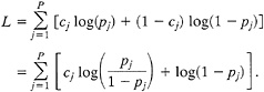
[3]

Under a few simple assumptions, L will be normally distributed with a mean and variance readily calculable from Eq. 3. Alternatively, simulated catalogs c_j may be constructed as described above, and the distribution of L may be estimated by the simulated sample distribution. The hypothesis test is made by comparing the value of L, using the actual earthquake record, with the distribution of simulated catalogs. If L for the actual catalog is less than 95% of the simulated values, then the hypothesis should be rejected. The L test may be applied to both the test hypothesis and the null hypothesis separately. Either, neither, or both might be rejected.

(iii) The “R test,” based on the ratio of the likelihood value of the test hypothesis to that of the null hypothesis. The log of this ratio is

[4]

R is the difference between two log-likelihood functions, with the test hypothesis having the positive sign and the null hypothesis the negative sign. Thus, positive values favor the test hypothesis, and negative values favor the null hypothesis. The hypothesis test involves calculating the distributions of R for the test hypothesis (that is, assuming that c_j is a sample of the process with probabilities p_j), and for the null hypothesis (assuming the c_j correspond to p_j). The log-likelihood ratio will be normally distributed if the log-likelihood functions for both the test and null hypotheses, calculated using Eq. 3, are normally distributed. Alternatively, the distributions may be calculated as follows: First, generate simulated catalogs using the probabilities p_j. Then compute the log-likelihood ratio for each catalog using Eq. 4 and compute the sample distribution of log-likelihood values. Now generate a suite of simulated catalogs using p_0j, the probabilities for the null hypothesis. For each of these, calculate R from Eq. 4 and compute their distribution. Again, two critical values may be calculated. Let R₁ be the least value of R, such that less than 5% of the catalogs simulated using the null hypothesis have a larger value of R. Then the null hypothesis can be rejected with 95% confidence if the actual value of R exceeds R₁. Let R₂ be the largest value of R, such that 5% or less of the catalogs simulated using the test hypothesis have a smaller value of R. Then the test hypothesis can be rejected with 95% confidence if the actual value of R is less than R₂. As in the other tests, either, neither, or both of the two hypotheses may fail the test.

Let us now revisit the topic of predictions in which no probability is given for the test hypothesis. These might be interpreted as identifying regions for which the probability of an earthquake is larger than that for other regions or in which the ratio of probability according to the test hypothesis to that of the null hypothesis is especially high. These predictions are often discussed in terms of a trade-off curve, in which the fraction of earthquakes predicted is compared to the fraction of space-time for which “alarms” are active. As more of time-space is covered by predictions, more earthquakes will be successfully predicted. Success of a prediction scheme is measured by comparing it with a hypothetical scheme which occupies the same proportion of space-time. An optimum threshold can be calculated if costs can be assigned to maintaining a state of alert and to unpredicted earthquakes. However, if probabilities are given for each region, then a prediction scheme can be tested using all of the probabilities, and there is no need to establish a threshold for declaring alerts. This separates the problem of testing scientific hypotheses from the policy problem of how to respond to predictions.

Predictions based on subdividing magnitude-time-space into regions have the disadvantage that probabilities may differ strongly from one region to another, so the success or failure of a hypothesis may depend strongly on small errors in location or magnitude estimates. Furthermore, earthquakes that occur just outside the boundaries of a high probability region pose a strong temptation to bend the boundaries or adjust the earthquake data. Statistical procedures should account for uncertainty in measurement and for imperfect specificity in stating hypotheses. One way to achieve these goals is to formulate hypotheses in terms of smaller regions, allowing for some smoothing of probability from one region to another. In fact, many prediction hypotheses lend themselves to description in terms of continuous variables, such as functions of distance from previous earthquakes or locations of geophysical anomalies. Let us consider a refinement of the “region” concept to include infinitesimal regions of time-space, in which p_j=∧ (x_j, y_j, t_j, m_j) dx dy dt dm. Here dx, dy, dt, and dm are small increments of longitude, latitude, time, and magnitude, respectively. The function ∧ is often referred to in the statistical literature as the “conditional intensity,” but I will use the notation “conditional rate density” to avoid confusion with the seismic intensity. The term “conditional” is used because earthquake prediction usually refers to a temporal increase in earthquake likelihood inferred from the existence of some special geophysical circumstance. If dx dy dt dm is made arbitrarily small, then 1−p_j approaches 1, and log(1−p_j) approaches −pj. After some algebra, we then obtain

[5]

where N is the number of earthquakes that actually occurred, N' is the total number of earthquakes predicted by the test hypothesis, and N′₀ is the total number of earthquakes predicted by the null hypothesis. The sum is over those earthquakes that actually occurred.

A consequence of shrinking the regions to an infinitesimal size is that there is no longer any reason to distinguish between the first and later earthquakes in a region; all of the regions are so small that the probability of a second event in a given box is also infinitesimal. Another consequence is that aftershocks must be dealt with carefully. No longer is it possible to assume that they will be unimportant if we consider only the first

qualifying earthquake in a region. Now it is virtually certain that the aftershocks from an earthquake in one region will occur in another. One way to deal with aftershocks is to use a declustered catalog in making the test. Another is to build aftershock prediction into both the test and null hypotheses. Kagan and Knopoff (6) offer an algorithm for modeling the probability of earthquakes following an earlier quake. Testing a hypothesis on “new data”—that is, using a hypothesis formulated before the occurrence of the earthquakes on which it is tested—now requires that the hypothesis be updated very quickly following a significant earthquake. Rapid updating presents a practical problem, because accurate data on the occurrence of important earthquakes may not be available before significant aftershocks occur. One solution is to specify in advance the rules by which the hypothesis will be updated and let the updating be done automatically on the basis of preliminary information. A more careful evaluation of the hypothesis may be carried out later with revised data, as long as no adjustments are made except as specified by rules established in advance.

Introducing aftershocks into the model makes it more difficult to compute confidence limits for the log-likelihood ratio than would otherwise be the case. Because the rate density may change dramatically at some time unknown at the beginning of a test period, it is very difficult to compute even the expected numbers of events analytically unless the aftershock models are very simple.

Rhoades and Evison (7) give an example of a method, based on the occurrence of earthquake swarms, in which the prediction is formulated in terms of a conditional rate density. They are currently testing the method against a Poissonian null hypothesis in New Zealand and Japan. They update the conditional rate calculations to account for earthquakes as they happen. As discussed above, it is particularly difficult to establish confidence limits for this type of prediction experiment.

A fair test of an earthquake prediction hypothesis must involve an adequate null hypothesis that incorporates well-known features of earthquake occurrence. Most seismologists agree that earthquakes are clustered both in space and in time. Even along a major plate boundary, some regions are considerably more active than others. Foreshocks and aftershocks are manifestations of temporal clustering. Accounting for these phenomena quantitatively is easier said than done. Even a Poissonian null hypothesis requires that the-rate density be specified as a function of spatial variables, generally by smoothing past seismicity. Choices for the smoothing kernel, the time interval, and the magnitude distribution may determine how well the null hypothesis represents future seismicity, just as similar decisions will affect the performance of the test hypothesis. In many areas of the world, available earthquake catalogs are insufficiently complete to allow an accurate estimate of the background rate. Kagan and Jackson (8) constricted a global average seismicity model based on earthquakes since 1977 reported in the Harvard catalog of central moment tensors. They determined the optimum smoothing for each of several geographic regions and incorporated anisotropic smoothing to account for the tendency of earthquakes to occur along faults and plate boundaries. They did not incorporate aftershock occurrence into their model, and the available catalog covers a relatively short time span. In many areas, it may be advantageous to use older catalogs that include important large earthquakes, even though the data may be less accurate than that in more recent catalogs. To date, there is no comprehensive treatment of spatially and temporally varying seismicity that can be readily adapted as a null hypothesis.

Binary (on/off) predictions can be derived from statements of conditional probability within regions of magnitude-time-space, which can in turn be derived from a specification of the conditional rate density. Thus, the conditional rate density contains the most information. Predictions specified in this form are no more difficult to test than other predictions, so earthquake predictions should be expressed as conditional rate densities whenever possible.

I thank Yan Kagan, David Vere-Jones, Frank Evison, and David Rhoades for useful discussions on these ideas. This work was supported by U.S. Geological Survey Grant 1434–94-G-2425 and by the Southern California Earthquake Center through P.O. 566259 from the University of Southern California. This is Southern California Earthquake Center contribution no. 321.

1. Bakun, W.H. & Lindh, A.G. (1985) Science 229, 619–624.

2. Keilis-borok, V.I. & Kossobokov, V.G. (1990) Phys. Earth Planet. Inter. 61, 73–83.

3. Kagan, Y.Y. & Jackson, D.D. (1995) J. Geophys. Res. 100, 3943–3959.

4. Nishenko, S.P. (1991) Pure Applied Geophys. 135, 169–259.

5. Papadimitriou, E.E. & Papazaehos, B.C. (1994) J. Geophys. Res. 99, 15387–15398.

6. Kagan, Y.Y. & Knopoff, L. (1987) Science 263, 1563–1567.

7. Rhoades, D.A. & Evison, F.F. (1993) Geophys. J. Int. 113, 371–381.

8. Kagan, Y.Y. & Jackson, D.D. (1994) J. Geophys. Res. 99, 13685–13700.