
Appendix B
Modeling
RATIONALE
In Chapters 4-8, which describe time-dependent gravity, we discuss a number of geophysical processes and their effects on the geoid. We attempt to assess whether those effects would be detectable with the generic missions described in Chapter 2. In this Appendix we describe the methods and geophysical models used to address these questions.
To determine whether the effects of a geophysical process are large enough to be detected, we first estimate the geoidal perturbation caused by that process. Suppose the process perturbs the gravitational potential at co-latitude θ and longitude ϕ by the amount δV(θ, ϕ). The resulting geoid anomaly is given by N(θ, ϕ)=δ V(θ, ϕ)/g, where g is the gravitational acceleration at the Earth's surface and is approximately g = GM/a2. With the notation shown in (Al 1), the geoid perturbation has the form
(B1)
where clm and slm are dimensionless coefficients and Hl,m,n are defined in (A5).
Once we have computed the clm and slm for a specific geophysical process (see B2 below), we construct the degree amplitudes, ![]() and compare them against the expected degree amplitude uncertainties described in Chapter 2 above. For several processes (e.g., post-glacial rebound, oceanographic fluctuations, changes in ground and surface water/snow/ice), the degree amplitude of the signal stands well above the degree amplitude uncertainties of generic SST and SSI missions at low degrees, indicating that those processes are readily detectable with those missions.
and compare them against the expected degree amplitude uncertainties described in Chapter 2 above. For several processes (e.g., post-glacial rebound, oceanographic fluctuations, changes in ground and surface water/snow/ice), the degree amplitude of the signal stands well above the degree amplitude uncertainties of generic SST and SSI missions at low degrees, indicating that those processes are readily detectable with those missions.
A degree amplitude comparison, however, is not always the most meaningful way to assess the resolving power of a mission. For example, the effects of processes with well-known spatial patterns could be detected, even though the degree amplitude is smaller than the expected satellite uncertainties. In that case, we can fit the spatial pattern of the geoid to the data to obtain the amplitude. This approach involves expanding the geoid pattern as a sum of spherical harmonics, and then fitting an overall amplitude of that sum to the spherical harmonic coefficients determined from the satellite data. Since the satellite errors for the individual coefficients are likely to be uncorrelated, the formal error for the fitted amplitude tends to
decrease as 1/√N, where N is the number of coefficients that make important contributions to the spatial pattern.
There are many processes where the spatial pattern can be approximated as a uniform mass change over a surface disc of known radius. In those cases, it is convenient to pose the issue in a somewhat different (though equivalent) form, and ask how well a satellite gravity mission can determine the change in surface mass averaged over the disc. As discussed in Chapter 2 and Appendix A, however, a gravity mission can provide a better result if the averaging kernel is a Gaussian weighting function over the entire Earth, with a full-width half maximum equal to the disc's diameter (rather than equal to 1 across the disc and 0 outside of it).
CALCULATIONS
It is straightforward to calculate the geoid perturbation caused by an arbitrary surface mass distribution with mass/area = σ(θ, ϕ). The geoid perturbation is defined as the gravitational potential due to this mass, divided by g (= 9.8 m/s2; the unperturbed gravitational acceleration at the Earth's surface). By expanding σ into spherical harmonics, finding the gravitational potential from each individual harmonic, and then arranging the result into the form (B1), we obtain
(B2)
where kl is the load Love number of degree l, ρave is the average density of the Earth (5517 kg/m3), and i = √( - 1). The Love number kl is included to represent the instantaneous elastic response of the solid Earth to the applied load. The Earth's non-elastic response, which is not included in (B2), depends on the time history of the load and is important only for loads that change at temporal scales of many centuries and longer. The only such loads considered in this report are large-scale continental ice sheets. The computation of the Earth's visco-elastic response to slow changes in the ice sheets is difficult, and must be done separately.
The result (B2) can be used to estimate degree amplitudes ![]() from an assumed mass distribution, which can then be compared with the expected satellite degree amplitudes. B2 can also be used to construct accuracy-versus-resolution estimates for a surface mass disc. To accomplish this, we expand the surface mass distribution in a form equivalent to the geoid expansion (B1):
from an assumed mass distribution, which can then be compared with the expected satellite degree amplitudes. B2 can also be used to construct accuracy-versus-resolution estimates for a surface mass disc. To accomplish this, we expand the surface mass distribution in a form equivalent to the geoid expansion (B1):
(B3)
where ρw is the density of water (assumed to be 1000 kg/m3), and is included in (B3) so that ![]() and
and![]() are dimensionless coefficients describing the spherical harmonic expansion of the surface mass expressed in the thickness of an equivalent mass of water. This is a useful measure of surface mass, because most of the surface processes for which accuracy-versus-resolution results are useful involve changes in water, ice, or snow.
are dimensionless coefficients describing the spherical harmonic expansion of the surface mass expressed in the thickness of an equivalent mass of water. This is a useful measure of surface mass, because most of the surface processes for which accuracy-versus-resolution results are useful involve changes in water, ice, or snow.
The orthogonality properties of the Hl,m,n (see A6) can be used to infer from (B3) that
(B4)
So, by comparing (B4) with (B2), we conclude that
(B5)
Equation (B5) can be used to transform geoid expansion coefficients clm and slm to mass expansion coefficients, and to construct degree amplitudes of the mass distribution in equivalent water thickness Several figures in the text (e.g., Figures 4.5, 4.6, 7.3, and 8.1) compare the mass degree amplitudes estimated by using assumed mass distributions in (B4), with the expected mass degree amplitudes of the satellite errors, which were computed using (B5) and the estimates of the geoid degree amplitudes described in Chapter 2. These comparisons are fundamentally equivalent to comparisons of the geoid degree amplitudes, and are included above only because the mass anomaly is often of greater direct interest than the geoid when interpreting the observations.
The mass degree amplitudes of the satellite errors can be used to estimate the accuracy-versus-resolution of the generic satellite missions. We use the geoid degree amplitudes described in Chapter 2, transform them to mass degree amplitudes using (B5), and use the results to estimate accuracy-versus-resolution as described in Appendix A, except that here we do not apply the constraint that the degree amplitude error not exceed the EGM96 error, since the EGM96 model does not provide information on the time-dependent gravity field. We do, however, use the GPS degree errors in constructing the SGG and SGGE accuracy-versus-resolution estimates, whenever the GPS degree errors are smaller than the SGG degree errors (see Chapter 2). The results are shown in Figures B.1-B.4. These figures are similar to the results shown in Figures 2.7 and 2.10, except that Figures B.1-B.4 are for surface mass, in water-equivalent thickness.
The degree amplitude and accuracy-versus-resolution results described in Chapter 2 are pertinent to 90-day geoid averages. Many of the time-dependent processes considered in this report are dominated by components that vary on seasonal or longer time scales. We use the 90-day uncertainty estimates to infer uncertainties of annually-varying and secular terms in the geoid by assuming that those terms would be least-squares fitted to the 90-day values. Using our estimates for the co-variance matrix of 90-day values, we can infer the uncertainties we would obtain for each individual temporal term using standard statistical arguments (see, for example, section 15.6 of Press et al., 1992). For example, if we were simultaneously to fit cos (wt), sin(wt), t, and a constant term to N days of data (where w = 1 cycle per year), we would obtain uncertainties for both the cos (wt) and sin(wt) terms equal to sv(2*90/N), where s is the 90-day uncertainty. Our uncertainty for the secular term would be approximately (s/N) v (12/N), in units of s/day. These transformations are used when estimating the annually-varying and secular components of the satellite degree amplitudes, both for the degree amplitude figures and for the accuracy-versus-resolution figures in the text.
SPECIFIC APPLICATIONS
These accuracy-versus-resolution results are particularly useful for estimating what changes in the thickness of disc-shaped mass anomalies can be resolved. Examples of disc-shaped anomalies considered in this report are the Antarctic drainage into the east side of the Ross Ice Shelf (estimated from Bentley and Giovinetto, 1991); seasonal, interannual, and secular changes in the Antarctic and Greenland ice masses (the non-secular variability was estimated from Bromwich et al., 1993, 1995, and the secular trend was estimated from the IPCC limits described by Warrick et al., 1996); continental glacier systems (ice-thickness changes from Meier, 1984); certain atmospheric processes, such as mid-latitude cyclones and large-scale precipitation events (with temporal and spatial scales taken from Holton, 1979); and individual aquifers and river drainage systems.
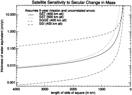
FIGURE B.1 Accuracy versus resolution for secular variations in the thickness of a disc of water, for four generic missions. We assumed a 5-year mission at an altitude of 400 km, which is probably realistic for SST and SSI, but is decidedly too long for an SGG mission, even at 400-km altitude. We denote the extended SGG mission as SGGE. The results here are used throughout the text to estimate the accuracies with which these missions could constrain various geophysical processes.
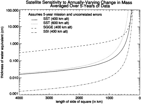
FIGURE B.2 Accuracy versus resolution for an annually-varying change in the thickness of a disc of water, averaged over 5 years, for four generic missions. The mission altitudes and durations are the same as in Figure B.1.
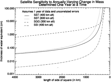
FIGURE B.3 Accuracy versus resolution for an annually-varying change in thickness of a disc of water, averaged over 1 year of data, for four generic missions. We assumed a 1-year mission and a 300-km altitude for SGG, since that is the most probable altitude for such a mission. We also include results for an SST mission at 600-km altitude to demonstrate the effects of an increase in altitude.
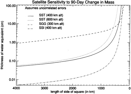
FIGURE B.4 Accuracy versus resolution for each 90-day value of the thickness of a disc of water for four generic missions. The mission altitudes are the same as in Figure B.3, but the values are calculated for a 90-day mission.
On the other hand, several important surface loads have geometries that cannot be characterized as discs. In those cases, we compute the geopotential coefficients by using estimates of the surface mass density as a function of latitude and longitude (i.e., s(θ, ϕ)) in (B2). Examples of these processes include global sea-level rise, oceanographic disturbances, atmospheric pressure variations, and continental water storage. The global sea-level rise was computed using the 5-minute topography of ETOPO-5 from Smith (1993) to determine the ocean/continent boundary. Oceanographic disturbances, such as deep ocean circulation, were determined using salinity, temperature, and sea-surface height from the Los Alamos POP general circulation model described by Dukowicz and Smith (1994), with model integration results provided by Frank Bryan at the National Center for Atmospheric Research. The effects of atmospheric pressure variations were calculated using the archived analysis fields of the National Centers for Environmental Prediction (formerly the National Meteorological Center) and ECMWF. Finally, temporal changes in continental water storage were calculated using a global soil-moisture data set from 1979-1993, generated as described by Huang et al. (1996) for a longer time period over the United States alone.
Finally, some processes, such as post-glacial rebound, cannot be represented as surface loads and their effects on the geoid must be modeled separately. Post-glacial rebound was modeled using the ICE-3G Pleistocene ice model of Tushingham and Peltier (1991) and the viscous-load Green's functions of Han and Wahr (1995). The viscous Green's functions were also used to estimate the visco-elastic response of the Earth to possible changes in Antarctic and Greenland ice since the Pleistocene. For example, we assumed that the Antarctic ice sheet has been melting at a steady rate (usually taken to be equivalent to 1 mm/yr of global sea-level rise) from time T in the past, until the present. We constructed a series of such models for different values of T. We then used the visco-elastic decay times and Green's functions from Han and Wahr (1995) to estimate the Earth's present-day visco-elastic response to each of these past changes in ice load. This allowed us to assess the problems of separating the effects of present-day changes in ice from the effects of the Earth's visco-elastic response to past events.


