
7
Sea-Level Change
Climate models used to study the effects of atmospheric greenhouse gases predict an overall increase in the global temperature during the next century of 1 to 3.5° C (Warrick et al., 1996). An increase of this magnitude could have numerous catastrophic effects, not the least of which would be caused by a substantial rise in global sea level due to a combination of melting glaciers and polar ice sheets and thermal expansion of sea water (Box 7.1).
Tide-gauge data show that sea level is already rising at a rate of between 1.0 and 2.5 mm/yr averaged over the past century (Warrick et al., 1996). The sources of this sea-level rise are not well understood, however. Estimates of various effects are included in Table 7.1. Most of the likely mechanisms involve the transfer of mass from the continents to the ocean basins. This mass redistribution would cause a secular perturbation in the geoid. The thermal expansion effect, however, involves no horizontal transfer of mass and so has no associated geoidal signal.
Satellite observations of time-dependent gravity could constrain changes in global sea-level in two ways. First, they could help identify the continental sources of water transferring into the ocean, through monitoring of the mass of ice sheets, continental glaciers, and groundwater aquifers. Second, they could be used to help identify the thermal-expansion component of sea-level rise by using the observations to solve directly for the mass increase in the ocean. These applications are discussed below.
THERMAL EXPANSION OF THE OCEANS
By comparing satellite gravity observations with tide-gauge or altimeter results over the time-span of the mission, it should be possible to discriminate between a mass influx, which affects both sea level and gravity, and thermal expansion, which affects only sea level. The contribution of thermal expansion to global sea-level rise is estimated to be between 0.2 and 0.7 mm/yr averaged over this century (Table 7.1). To improve the determination of this component, a gravity satellite would need the capability to detect a sea-level rise with an accuracy on the order of a few tenths of a mm/yr. This would constrain the total mass influx more closely for each year that the gravity data are available. Separating the relative contributions among the four sources listed in Table 7.1 will also require a gravity mission of some years.
Figure 7.2 shows the predicted secular geoid perturbation caused by a 1 mm/yr rise in sea level, assuming that the rise is due entirely to an increase in water mass (the geoid in Figure 7.2 changes over the continents because a spatial constant has been removed from the output at each time step: i.e., the mass of the Earth, as a whole, is assumed to be conserved). Note that the geoid amplitudes are small, no more than a few hundredths of a mm/yr. The signal caused by a rise of a few tenths of a mm/yr would be smaller still. This will be a difficult signal to detect.
|
Box 7.1 Impact of Global Sea-Level Rise A large fraction of the Earth's total population resides close to sea level, and few societies would remain unscathed by the global agricultural and industrial effects of a rise of sea level by I m or more. Half of the world's megacities (population >8 million) are located near sea level with a total yea 2000 population exceeding 150 million, and these constitute but a small fraction of the ports and communities that thrive globally on coastal commerce, agriculture, and industry. An estimated 46 million people per year are at risk of flooding due to storm surges, and a l-m rise in sea level would raise that number to 118 million people per year (IPCC, 1996). A rise in sea level has its greatest effects on low-lying regions that slope gently inland (e.g., Florida and Indonesia with 15% of the world's coastlines) or are on the flood plains of large river systems (eg., Rhine, Ganges, Nile, Mekong). In these areas, a rise in sea level triggers landward transgression of the coastline and subsurface incursion into fresh water reservoirs, resulting in a loss of arable land. By the year 2100, a 1-m rise in sea level could lead to land loss ranging from 0.05% in Uruguay, 1.0% in Egypt, 6% in The Netherlands, and 17.5% in Bangladesh to 80% in the Marshall Islands (IPCC, 1996). In the United States, it has been estimated that a rise in sea level by 1 m would drown 20-85% of coastal wetlands and would result in coastal encroachment of up to 7,000 square miles, an area the size of Massachusetts (Titus et al., 1991). The loss of coastal ecosystems would also have negative effects on tourism, infrastructure, freshwater supplies, biodiversity, and fisheries. In Blackwater National Wildlife Refuge of the Chesapeake Bay, for example, sea-level rise has resulted in the inundation of a significant fraction of marshland (Figure 7.1), altering the ecological balance of the area With regard to infrastructure, more than 90% of all power stations in the United States are located close to the coasts; so also are many industrial complexes, to he within easy reach of harbors and raw materials. For many nations, economic losses caused by sea-level rise could exceed 10% of their Gross Domestic Product (IPCC, 1996). The social impact of large communities migrating inland and the economic costs of increased sea-level defenses are likely to have adverse effects throughout coastal societies. The current global sea-level trend is a rise of approximately 0.2 m/century, but it is possible that this could be accelerated by a factor of 3-5 by global warming trends, although smaller rates of acceleration are more likely. Current rates, if they remain constant, are slow enough to permit appropriate societal responses to sea-level rise. However, an acceleration by a factor of 5 would affect low-lying areas at rates that would require more immediate remedial action by coastal societies, so early detection of an acceleration is an important planning requirement. |
TABLE 7.1 Estimated Ranges of Likely Contributions to Sea-Level Rise, Averaged over the Past 100 Years (from Warrick et al., 1996)
|
Contribution |
Rate of Increase or Decrease (mm/yr) |
|
Thermal expansion |
0.2 to 0.7 |
|
Antarctica |
-1.4 to 1.4 |
|
Greenland |
-0.4 to 0.4 |
|
Glaciers and small ice caps |
0.2 to 0.5 |
|
Surface and groundwater |
-0.5 to 0.7 |
The degree amplitudes from a 1 mm/yr rise in sea level do exceed (slightly) the 5-year, 400-km SST-mission uncertainties for l < 6 (see Figure 7.3). Because the pattern of the geoid signal is well known in this case (shown in Figure 7.2), it might be possible to obtain a useful estimate for the amplitude of this effect by fitting that pattern to the satellite data. Using the uncertainties described in Chapter 2, we find that data from the 5-year SST mission would provide a 1-sigma error on the mass contribution to sea level of about 0.1 mm/yr. The results obtainable with an SSI mission would have even smaller formal errors—the effects of a 1 mm/year change in sea-level rise above the SSI errors at degrees all the way up to 1 = 20
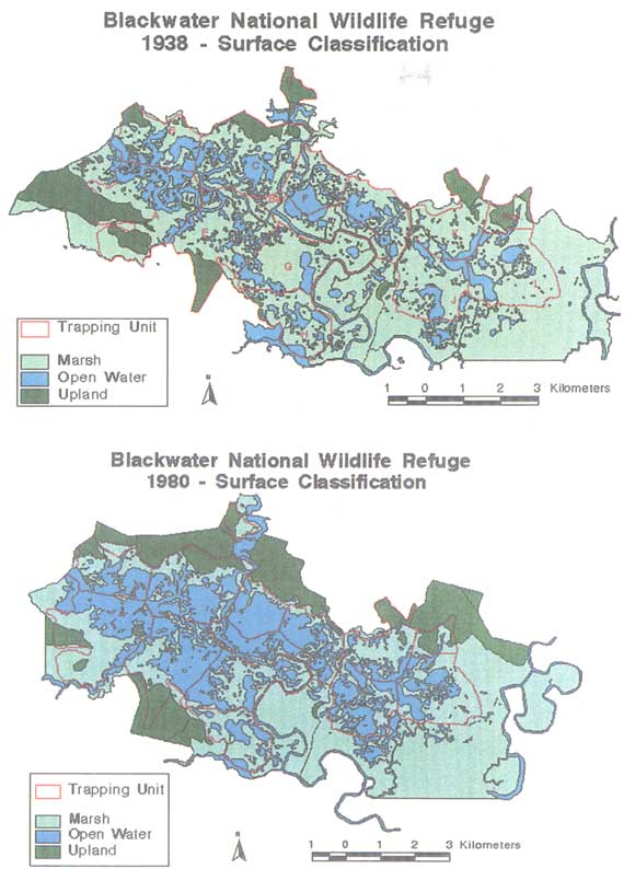
FIGURE 7.1 Changes in marsh and upland (higher ground) land types in Blackwater National WildlifeRefuge, Chesapeake Bay, Maryland due, in part, to sea-level rise. From 1938 to 1980,an average of 17.3 hectares/yr of marsh was inundated. Figure based on aerial photography and prepared under the auspices of NOAA's Coastal Change Analysis Program. Courtesy of C. Stevenson, University of Maryland Center for Environmental and Estuarine Studies.
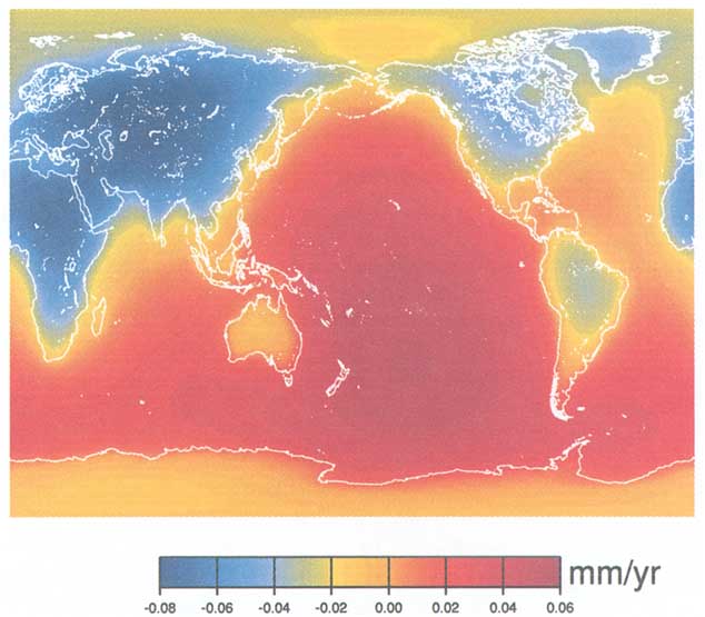
FIGURE 7.2 The secular change in the geoid caused by a 1 mm/yr rise in global sea level, assuming that sea-level rise is due entirely to an increase in water mass. The spatial mean is set to zero, consistentwith the assumption that the Earth as a whole conserves mass.
(Figure 7.3, bottom panel). But problems of separating the global sea-level signal from the effects of other secular geophysical signals are likely to limit the sea-level accuracies to about 0.1 mm/yr in any case. (An SGG mission, even the extended-duration SGGE mission, is not sufficiently accurate at low degrees to be useful for this application.) An accuracy of 0.1 mm/yr could, indeed, be useful in separating the thermal expansion effects from the effects of an increase in mass, provided that the total global sea-level rise has been measured to this same high accuracy using some other technique (satellite altimetry, for example), during the same time period. Note that any conclusions obtained from this study would be based on data from the limited time-span of a satellite mission (nominally assumed throughout this report to be about five years) and might not reflect true long-term trends. A long-term monitoring capability would be desirable.
In addition to providing information on global and regional sea-level rise, satellite gravity data could be used to study changes on basin scales. For example, sea level in the North Atlantic is believed to have risen by 3 cm between 1994 and 1995, with much of the increase occurring over a few months (Figure 7.4)
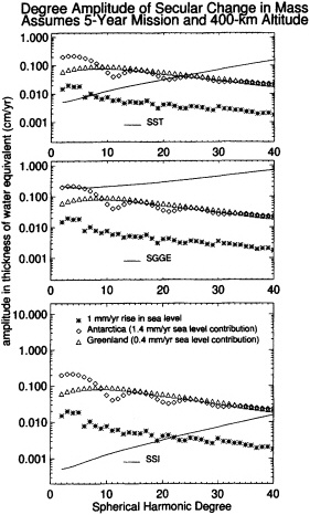
FIGURE 7.3 The degree amplitudes for secular fluctuations in geoid, compared with the expected uncertainties for 5-year SST, SGGE, and SSI missions at 400-km altitude. The geophysical processes considered here include post-glacial-rebound (for the entire globe: North America, Scandinavia, Greenland, and Antarctica; and assuming a lower-mantle viscosity of 10.E21 Pa-sec); present-day changes in Antarctic and Greenland ice, at a level to cause a global sea-level change of 1.4 mm/yr for Antarctica and 0.4 mm/yr for Greenland, which are the upper bounds from Warrick et al. (1996); and a 1 mm/yr change in global sea level, assuming that this is entirely due to the transport of mass between the oceans and continents.
(Carton and Miller, 1997). This increase, which should be readily detectable by an SST or SSI mission (cf. Figure B.3 in Appendix B), was associated with an anomalous warming of surface temperatures and changes in the structure of the thermocline. For identifying the causes of such basin-scale anomalies, a vitally needed piece of information is the relative contribution of thermal expansion compared with an overall increase in mass. Thus again, satellite measurements of the increase in mass would be invaluable in sorting out the causes of sea-level rise.
ICE MASS BALANCE
The masses of glaciers, ice caps, and ice sheets (the term ''ice sheet" is reserved for the vast ice covers of Antarctica and Greenland) vary temporally through the exchange of water with the oceans. These ice bodies on land can shrink in two ways—by excess melting and liquid water runoff and by breaking off as icebergs. In either case the mass lost soon reaches the ocean. Conversely, ice bodies can gain mass only by an excess of snowfall on their surfaces; the moisture source is evaporation from the oceans. Thus, the measurement of the total mass balance (deviation from constant mass through time) of the ice on land is a direct, though partial, measure of the changes of water mass in the oceans.
There are two important advantages of gravity measurements for large-scale mass-balance studies. The first is that, since gravity depends simply on mass, changes in gravity provide a direct measure of ice-mass balance that is independent of changes in the mean density of the ice bodies, which can change with time. Secondly, gravity serves as an automatic integrating tool, thus obviating the huge difficulty that glaciologists face in extrapolating results from field studies in a few areas to much larger regions, especially to the entirety of the vast ice sheets. For both these reasons, glaciologists eagerly await future satellite-gravity missions.
Contributions from the Greenland and Antarctic Ice Sheets
Currently, the large-scale mass balances of Greenland and Antarctica are poorly known. Estimates of their contributions to the global sea-level rise during this century are in the range of ± 1.4 mm/yr for Antarctica and ± 0.4 mm/yr for Greenland (Table 7.1)—not even the sign is known. Both upper bounds correspond to geoid amplitudes of 2.0 to 2.5 mm/yr, spread over the respective ice sheets.
Figure 7.3 shows the degree amplitudes of a uniform change in mass of each sheet, assuming the
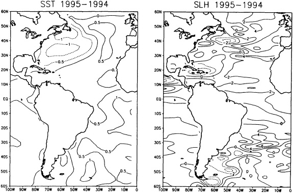
FIGURE 7.4 Observed change in annual averaged sea level in cm (right-hand panel) and sea-surface temperature in degrees C (left-hand panel) for 1995 relative to 1994. The warm El Niño conditions of the tropical Pacific have receded, causing sea level to drop. In the eastern North Atlantic, a warming of sea-surface temperature is reflected in a rise of sea level.
mass changes are equal to the upper bounds cited by Warrick et al. (1996). These results include the effects of the Earth's elastic response to the changes in ice load, as described in Appendix B. Note that the results rise well above the uncertainties for a 5-year SST mission at values of l below 25 (corresponding to half-wavelengths greater than 800 km), and for a 5-year SSI mission at values of l below 40 (half-wavelengths greater than 500 km). Approximating Antarctica and Greenland as squares about 3500 km and 1300 km on a side, respectively, we estimate from Figure B.1 that a 5-year, 400-km altitude SST mission would be sensitive to changes in the overall mass of Greenland and Antarctica to an accuracy corresponding to better than 0.01 mm/yr of sea-level rise for each ice sheet. (The water thickness results from Figure B.1 can be converted to sea level by multiplying by the ratio of the ice sheet area to the area of the world's oceans.) A 5-year SSI mission would be about an order of magnitude more sensitive.
It is important to note, however, that there are ambiguities in interpreting gravity signals over ice sheets because of problems in separating the effects of ice-sheet changes from the effects of isostatic rebound, interannual variations in snow accumulation rates, and atmospheric pressure. These problems are discussed in turn below.
Isostatic Rebound
It is difficult to distinguish between effects of present-day changes in ice-sheet mass and effects of the Earth's visco-elastic response to changes in ice mass over the past few hundred to several thousand years, particularly in Antarctica. In principle, one could correct for the isostatic uplift by measuring it on exposed rock. Although most of Antarctica is ice-covered, there are many exposures in the extensive Transantarctic Mountains, which cut through the continent from the Atlantic to the Pacific (Figure 7.5). Hence a campaign of GPS measurements along the Transantarctic Mountains (and some nuna-
taks elsewhere) to determine uplift rates would be a valuable undertaking. Accuracies on the order of 1-2 mm/yr (taking into account the poorer geometry and increased ionosphere delays in polar regions) should be attainable with five years of continuous GPS measurements. (Tectonic uplift rates in the Transantarctic Mountains could be as large as 1 mm/yr [Behrendt et al., 1991], but are more likely no more than a few tenths of a millimeter per year [Fitzgerald, 1994].) This corresponds to an uncertainty in the secular gravity signal that is equivalent to about 4 mm/yr of ice, or about 0.15 mm/yr of global sea-level rise. The problem is, however, that crustal uplift rates measured for the Transantarctic Mountains, which occupy only a small fraction of the total area of Antarctica, would likely not be representative of the average uplift rates for the entire continent. It is thus probable that the best use of such GPS measurements would be to help assess independent models of the rebound, which would then be used to remove the effects at all locations.
Rebound models in their current state of development would not suffice to solve the problem. Uncertainties in the Earth's viscosity profile and the time evolution of the Antarctic ice sheet correspond to uncertainties on the order of 30 mm/yr in present-day thickness changes of the Antarctic ice sheet, which is equivalent to about 1.2 mm/yr of global sea-level change. At first glance, this result suggests that a gravity mission would not improve the global sea-level change estimates of Warrick et al. (1996). However, it is likely that a dedicated gravity mission would lead to a solution for secular changes in the gravity field over northern Canada that would greatly improve our knowledge of the Earth's viscosity profile (see Chapter 5). In that case, the main source of uncertainty in the Antarctic visco-elastic change would be the detailed time evolution of the Antarctic ice sheet itself. The level of that uncertainty would depend on the Earth's viscosity profile. If the lower-mantle viscosity is 4.5 × 10²¹ Pa-sec or smaller, the uncertainty in the Antarctic contribution to present-day sea-level rise would probably be on the order of 0.6 mm/yr, with about equal contributions from uncertainties in the Pleistocene ice history and estimates of what the mass balance might have been over the past several hundred to several thousand years. At larger values of lower-mantle viscosity (e.g., 20 × 1021 Pa-sec or greater), the Earth would respond more slowly to past changes in ice, and the total uncertainty might be reduced to 0.3 mm/yr or smaller. Uncertainty estimates this small would indeed lead to improved estimates of the Antarctic contributions to sea-level change, though any such result would be representative of the ice sheet for only the relatively brief duration of the satellite mission.
Snow-Accumulation Rates
Another interpretation difficulty arises from the consideration of interannual variations in the rate of snow accumulation on the ice-sheet surfaces (Figure 7.5). Here the problem is not in determining the change in mass of the ice sheets, but in distinguishing between changes in the mass of the solid ice, which can occur only by ice-dynamic processes with time scales of decades to millennia and which, consequently, are of the greatest interest in terms of secular changes in sea level, and ephemeral changes associated with a few years of higher-than-normal or lower-than-normal snowfall rates. It is not well known how large the average variability in snowfall might be over an entire ice sheet, but on a more local scale an average interannual variability of 25% has been estimated for Antarctica (Giovinetto, 1964); a similar figure is likely for Greenland. (The interannual variability in outflow is much less than this because outflow is principally by solid ice discharge into the ocean.) Even if interannual variations were uncorrelated from year to year, which is climatologically unlikely, this would yield an error in estimating the secular change in ice mass from a 5-year mission that would be on the order of 10% of the annual mass input, or approximately 18 mm of ice, equivalent to 0.6 mm/yr of sea-level change, for Antarctica, and 70 mm of ice (0.3 mm/yr sea-level equivalent) for Greenland. An error of this magnitude would be a serious hindrance in determining the true, long-term contribution of the ice sheet to sea-level change.
Fortunately, this error can be reduced in two ways. The first is by the calculation of broadly averaged snowfall rates from the atmospheric-moisture-flux divergences over the ice sheets determined from atmospheric numerical analyses that incorporate satellite-based soundings of water vapor and winds over the surrounding oceans, as well as regular rawinsonde observations from a small number of surface stations. Meteorologists expect that by the year 2000 the total input can be known to ± 10% for Antarctica and a few percent for Greenland (D.H. Bromwich, personal communication). Furthermore, a substantial portion of the uncertainties would be systematic, i.e., not varying from year to year. Thus the error in the interannual differences from a long-term mean could be less than 10% of the total input; if it were half that, the combined error for Antarctica and
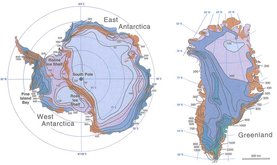
FIGURE 7.5 Map of the ice sheets, showing mean annual accumulation rates in kg/m2 yr. The contourinterval is 100 kg/m2 yr, with additional contours at 50 kg/n 150 kg/m2 yr in Antarctica (left). Colors change at accumulation rates of 100, 200, and 400 kg/m2 yr in Antarctica and 100, 200, 500, and 9900 kg/m2 Greenland Brown zones are mountainous regions with extensive exposed rock. The Transantarctic Mountains cut across Antarctica between the South Pole and the two great ice and divide the continent into East Antarctica and West Antarctica. The latitude lines provide the scale for Antarctica—10° of latitude equals 1100 km. Note that the s Antarctica and Greenland differ by about a factor of two; Greenland is comparable in size to East Antarctica.
Greenland could be reduced to 10 mm/yr of ice (0.3 mm/yr in sea level).
Secondly, the gravity measurements themselves can help determine the interannual variations, at least for the period of the mission. According to our calculation, geoid amplitudes could well vary by 1 mm or more over both Antarctica and Greenland (Figure 1.2), if average interannual thickness changes, in water equivalent, were about 18 mm for Antarctica and 70 mm for Greenland. We conclude from Figure B.2 that an SST mission at an altitude of 400 km could in principle resolve these thickness variations to an accuracy of about 0.3 mm and 1.0 mm for Antarctica and Greenland, respectively. For a nominal SSI mission, those numbers are 0.08 mm for Antarctica and 0.1 mm for Greenland, but in actuality the accuracy will be less, because the gravity signal of the ice sheet is contaminated by the signal from the surrounding ocean and by the atmospheric pressure over the ice sheet itself. We estimate, using the annually-varying geoid predicted from the ocean general circulation data described in Chapter 4, that the oceanic effects could limit the accuracy in determining interannual changes in snowfall to about 2 mm (0.07 mm of sea level) for Antarctica and about 10 mm (0.04 mm of sea level) for Greenland. This still would represent a great improvement over current methods of determining changes in snowfall over time. We consider the effect of atmospheric pressure next.
Atmospheric Pressure
Yet another problem arises, particularly in Antarctica, from the fact that the gravity satellite will sense the mass of the atmosphere as well as the masses of the ice sheet and the solid Earth. The mean atmospheric pressure over the ice sheet (which reflects the overlying mass) must be determined from a very small number of measuring points; consequently there may be an error as large as 1 mbar (about equal to 10 mm of ice or 0.3 mm of sea-level equivalent) in evaluating annual averages. This could be a relatively static error, however, so it would not notably affect a calculation of secular change rates. There still remains a random-error component, which is on the order of a millibar on annual averages (Chen et al., 1997; D.H. Bromwich, personal communication), hence presumably is less than 0.5 mbar (5 mm of ice; 0.2 mm of sea level) with respect to secular change rates. The uncertainties in mean pressures can best be reduced by extending the number of automatic weather stations over the Antarctic surface and assuring that data from them are available and used in mean-pressure calculations. The situation is less serious in Greenland because Greenland is smaller and contains a better distribution of weather stations.
Complementarity with Satellite Laser Altimetry
Estimates of mass balance could be further improved if the present-day changes in the heights of the ice sheets could be determined separately using laser altimeter measurements from an orbiting satellite—specifically, NASA's planned Laser Altimetry Mission. For a given mass increase, the surface height changes would be in the ratio of 1:3.5:10 for isostatic uplift, changes in solid ice, and changes in snow accumulation at the surface, respectively, because the source of mass change in each of those cases is characterized by a different mean density. If the cause were atmospheric pressure changes there would be no change in height at all (the response of the ice to pressure fluctuations is negligible). It follows that measurements of both change in height and change in gravity should, in principle, make it possible to distinguish between uplift and changes in mass of the ice sheet. NASA's planned Laser Altimetry Mission, carrying a laser altimeter in a 94° orbit with a nominal lifetime of 4 years, is designed to detect mean surface-height changes to better than 10 mm/yr; an accuracy of a few mm/yr in mean height change over large areas probably will be attained. An accuracy of 3 mm/yr, combined with the satellite gravity measurements, would make it possible to calculate the contribution of the ice sheet to sea-level change at the 0.1 mm/yr level. Neither satellite gravity nor satellite laser altimetry has that capability alone—the two types of measurement are strongly complementary. (The laser altimeter measurements are subject to most of the same uncertainties about causes as the gravity measurements, but with different sensitivities. Without better knowledge of the isostatic-rebound and snowfall-variation effects, such as could be obtained using satellite gravity, estimates from laser altimetry of the ice sheet contributions to sea level would probably be on the order of 0.2 mm/yr.)
Drainage Systems Within Ice Sheets
Ice sheets are complex composites of individual drainage systems or basins, some of which are characterized by fast-moving, low-gradient ice streams bordered by slowly flowing ice, some by huge outlet glaciers through peripheral mountain ranges, and some by broad expanses of open sheet flow with only small, local glaciers. Although from a direct societal standpoint the total mass balance of the ice on land is the most relevant quantity to measure, from a glaciological standpoint it is equally important to measure the mass
changes in individual drainage systems within the ice sheets, because they are the basic dynamic units; glaciologists can only learn how to predict future changes in ice-sheet mass balance by understanding the dynamics of these basic units. A complicating factor is that the dynamic behavior of a particular drainage system may be nearly independent of the dynamic behavior of even its nearest neighbors.
The ice sheets are so large that satellite gravity can provide a valuable approach to the study of subdivisions like individual drainage systems as well as entire ice sheets. For example, the mass of ice in the large drainage system that empties into the east side of the Ross Ice Shelf is suspected to have fluctuated dramatically in the past because of unstable dynamic behavior, including a rapid retreat at the end of the last ice age that may even be continuing at present, albeit at a reduced rate. Our gravity model indicates that secular changes in the thickness of this drainage system, which could be as large as 50 mm/yr of water equivalent, could cause a geoid change of up to 0.7 mm/yr over an approximate square of 600 km on a side. Using the method described in Appendix B for determining the resolving power of the different generic missions, we conclude that a 5-year SST mission flying at an altitude of 400 km could determine the secular change in ice thickness in this region to an accuracy of about 4 mm/yr. The determination of secular changes in the masses of this and other large drainage systems would allow models of ice-sheet dynamics to be tested.
Unfortunately, the same problems arise with the interpretation of gravity changes over a drainage system as with the interpretation of changes over the encompassing ice sheet as a whole, and the same approaches to alleviating those problems mostly apply. There is a special situation to note with respect to isostatic rebound, however. Isostatic rebound models, such as those based on the ICE4G model of Peltier (1994), that incorporate the results of analyses of ice-sheet dynamics, show an isostatic rebound rate on the east side of the Ross Ice Shelf in West Antarctica that is much greater than the Antarctic average because of the major modeled ice-sheet retreat there at the end of the last ice age. Modeled rebound rates greater than 10 mm/yr extend widely and the maximum rate is over 15 mm/yr. It is no coincidence that the highest modeled uplift rates are focused on the regions where the greatest likelihood of rapid change from a glaciological perspective exists today—it is the same high glaciological sensitivity of concern today that presumably led to large changes in ice mass in these areas in the past. As a 15 mm/yr rebound rate is gravitationally equivalent to an ice-thickness change of about 60 mm/yr, even a large glaciological imbalance could be obscured by ongoing isostatic uplift.
Fortunately, the Transantarctic Mountains cut through the regions showing large modeled uplift rates, so GPS surveys in those mountains of the type recommended above would provide an excellent check on the models. Furthermore, because the rates of change that might be attributed to either changing ice mass or isostatic rebound are so large, this region is particularly well suited to testing by comparing results from a gravity satellite with those from a satellite-borne laser altimeter.
Contributions from Glaciers
Satellite gravity could also be used to study secular, interannual, and seasonal changes in the mass balance of ice and snow in regions characterized by a concentration of a large number of glaciers and ice caps. These systems are important for inferring sea-level change because, even though their masses are much smaller than those of the ice sheets, they are capable of much more rapid response to climate change. Consequently, they may at present be contributing at least as much to sea-level change as the ice sheets (cf. Table 7.1).
An example of a large glacial system that could change sufficiently in mass to be detected by a gravity satellite is the system of glaciers that runs from the Kenai Peninsula in southern Alaska down along the Coastal Ranges of the Yukon and British Columbia. This region is characterized by unusually heavy snowfall, particularly in the winter; field observations suggest that the thickness of the glaciers varies annually with an amplitude of about 2.5 m water equivalent (Meier, 1984). This would produce a geoid signal that varies annually by as much as 20 mm over the region (an area equivalent to a square about 300 km on a side) (Figure 1.2). For comparison, we estimate from Figure B.2 that a 5-year SST mission at 400-km altitude could resolve such a system to an accuracy of about 0.5 m of water (about 1/5 of the total effect). For the nominal SSI mission, the accuracy is much better—about 5 mm (see Appendix B for a description of how these accuracies were estimated). The secular trend in this system could total about 0.4 m/yr of water equivalent (Meier, 1984), causing a geoid perturbation with an amplitude of 2-3 mm/yr over the same 300-km spatial scale. This could be resolvable with a 5-year, 400-km altitude SST mission to an accuracy of about 20 cm/yr water equiv-
alent, which is good enough to be useful for constraining the secular trend. For the SSI mission, the accuracy becomes 2 mm/yr. Although this glacier system is likely to have the largest annually-varying signal of any system around the world, there are other large glacier systems that could have comparable secular effects.
These estimates for the detection of the seasonal changes in glaciers are somewhat misleading, because there is also a large wintertime snowfall on the surrounding non-glaciated region and there is no good way of knowing what proportion of the seasonal signal to attribute to snow on the glaciers. A gravity mission would provide the total seasonal signal over the entire glaciated and non-glaciated region, which would help constrain estimates of the seasonal snowfall in the region. (Seasonal snow is not a problem on ice sheets because the area of exposed land is so small compared with the area of the ice sheet.)
CONCLUSIONS
-
The sources of global sea-level rise (measured by tide gauges to be between 1.0 and 2.5 mm/yr over the last century) are not well understood. Most of the likely mechanisms involve mass redistribution from the continents to the oceans; gravity measurements can give unique insights through the continual monitoring of geoid changes, not only on global scales, but also on regional and basin scales. From an SST type mission (5-yr mission assumed), accuracy of perhaps a tenth of a mm/yr is attainable.
-
The measurement and interpretation of changes in Greenland and Antarctica is a complex issue, given the complex nature of the phenomena involved: secular changes in ice-sheet mass, post-glacial rebound, interannual variability in snowfall, and the effect of atmospheric pressure trends.
-
Post-glacial rebound could be partly separated from ice changes using a network of GPS receivers on the land surface, numerical models of rebound that use improved determinations of mantle viscosity provided by the gravity mission, and comparisons with satellite laser altimetry.
-
Separation of interannual mass changes from true secular changes will be aided greatly by the continually improving calculations of mass input to the ice-sheet surfaces from measurements of moisture-flux divergence around the perimeters of the ice sheets.
-
The removal of pressure effects over Antarctica will become more effective as the number of automatic weather stations in the interior of the continent increases.
-
Gravity measurements would be most effective in combination with the observations planned for NASA's Laser Altimeter Mission. Together, an accuracy of 0.1 mm/yr in the determination of the contribution of the ice sheets to sea-level change should be attainable.
-
-
Satellite gravity measurements are capable of yielding valuable information about the mass balance of individual drainage systems within the Antarctic ice sheet, as well as of the ice sheet as a whole. Glaciologists could use such information to test models of ice dynamics, which are essential to the prediction of future sea-level change.
-
Satellite gravity could be used to study secular, interannual, and seasonal changes in the mass balance of ice and snow in regions characterized by a concentration of a large number of glaciers and ice caps. A prime example is the glacier system that runs from the Kenai Peninsula in southern Alaska down to the coastal ranges of the Yukon and British Columbia.
-
The need for long time series strongly favors SST- or SSI-type missions. SGG missions do not have enough accuracy at low degrees, nor do they have sufficient mission length.


