
Appendix A
Spherical Harmonics: Degree Variances, Wavelengths, Upward Continuation, Anomalous Potentials, Signal and Error Spectra, and Gaussian Averages
A.1 SPHERICAL HARMONIC EXPANSIONS OF GRAVITATIONAL POTENTIALS
In geodesy, the Earth's gravitational field is commonly expressed as an expansion in spherical harmonic functions. These functions arise when Laplace's equation (the fundamental differential equation of gravity) is solved in spherical coordinates. Gravitational potentials satisfy Laplace's equation in regions of free space, that is, where densities are zero; thus the spherical harmonic expansion of the Earth's gravity field is a useful device for describing the field outside the Earth, such as is felt by orbiting satellites. (One assumes that the entire mass of the atmosphere lies below the satellite for this purpose.)
The derivation of the spherical harmonics can be found in many books (e.g., Heiskanen and Moritz, 1967; MacRobert, 1967; Jackson, 1975; Sansone, 1991), so we merely sketch the pertinent results here. Choose a polar coordinate system with r the radial distance from the origin, θ the angular distance from the (''north") pole (the colatitude), and ϕ the longitude. Let V(r, θ,ϕ) be a gravitational potential satisfying Laplace's equation
(A1)
with the boundary conditions that it be finite and single valued for 0 ≤ θ ≤ π, 0 ≤ ϕ ≤ 2π, and that V → 0 as r → ∞. Define
(A2)
for non-negative integers m. Define the associated Legendre functions Pl,m(x) for integer l ≥ 0, integer m with 0 ≤ m ≤ l, and x in -1 ≤ x ≤ 1 by
(A3)
This definition is that of MacRobert (1967); some authors (e.g., Jackson, 1975) include a factor of (-1)m. Define normalization constants Al,m as
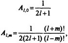
(A4)
then the "geodetically normalized surface spherical harmonics" (hereafter, "spherical harmonics") of degree I and order m may be defined as
(A5)
with n= 1,2 and the understanding that when m = 0, Hl,0,1(θ, ϕ) = (Al,o)−½Pl (cosθ) and Hl,0,2 is not used; thus, for a given l there are 2l + 1 spherical harmonics. The spherical harmonics so defined form an orthonormal set over the surface of a sphere, which means that
(A6)
The set is complete under the inner product norm, so that any function f(θ, ϕ) whose square is integrable over the surface of the unit sphere can be approximated by an expansion in spherical harmonics in such a way that the mean squared error of the infinite series expansion vanishes.
The solid spherical harmonic
(A7)
satisfies Laplace's equation (A1) and the boundary conditions, and therefore so also will the sum
(A8)
where al,m,bl,m are constant coefficients, provided that the infinite sum converges uniformly and sufficiently rapidly to permit term-by-term differentiation in (A1). For the twice differentiable functions such as V, such convergence has been established. Proofs can be found in Sansone (1991). In writing (A8) b1,o appears, although Hl,o,2 is not used; this is for convenience of notation. In what follows, such a coefficient should be taken to be zero.
If a gravitational potential is expanded in the form (A8), then the coefficients al,m, bl,m have the rather awkward dimensions of potential per unit length(l+l). In order to avoid this, geodesy uses a scaled version of (A8) which makes the constants dimensionless:
(A9)
Here, G is the Newtonian gravitational constant, M is the total mass of the Earth, and a is the equatorial semi-axis of the ellipsoid chosen as the reference shape of the Earth. The sum starts at l = 2 because the degree-one terms are made to vanish by taking the origin at the center of mass of the Earth. The degree-
zero term, GM/r, is explicitly factored out of the sum; it represents the potential of a spherically symmetric mass distribution. The remaining terms in the sum have coefficients cl,m,sl,m which are dimensionless fractions of the spherically symmetric potential on the surface r = a.
A.2 DEGREE VARIANCES
From the above it can be shown that the spherical harmonics Hl,m,n (θ,ϕ) have m zeros on meridians in π radians of longitude and l — m zeros on parallels in π radians of colatitude; thus the degree l ≥ 0 counts the total number of zero crossings in any hemisphere bounded by a meridian plane, while the order 0 ≤ m ≤ l counts how many of those zero crossings are along meridians. The (θ,ϕ) coordinates of a point on the sphere depend on what point has been chosen as the pole (θ = 0) and what half-plane has been chosen as the prime meridian (ϕ = 0). Therefore, the coefficients in a spherical harmonic expansion of a function depend on the choice of coordinates. However, there is a quantity, ![]() , called the "degree variance" and defined by
, called the "degree variance" and defined by
(A10)
which is constant for all choices of the coordinate system.
A.3 WAVELENGTH RELATED TO HARMONIC DEGREE
Physical properties that depend on distance but not on direction turn out to depend on 1 but not m, for the same reasons that the degree variances depend on 1 but not m. Although the spherical harmonics are functions on a two-dimensional surface, in discussions of isotropic phenomena it is convenient to characterize them by a one-dimensional "wavelength" λ1. Since Hl,m,n(θ, ϕ) has l zeros in π radians, λ1 istaken to be 2πa/l, where a is the semi-major axis of the Earth's reference ellipsoid or an average value for the radius of the Earth. This works out to λl ≅ (40,000 km)/l.
A.4 ATTENUATION WITH ALTITUDE
According to Newton's inverse-square law for the gravitational force, gravity fields decay with distance away from their sources. It turns out that this decay is dependent on wavelength, so that for any given distance away from the source, short-wavelength anomalies are attenuated more strongly than long-wavelength anomalies. The amount of attenuation depends on both the wavelength of the anomaly and the distance from the source. If V(a)(θ, ϕ) is the gravitational potential on the surface r = a with coefficients cl,m, sl,m
(A11)
then the gravitational potential on the surface r = a + h is
(A12)
Thus a satellite orbiting the Earth at an altitude h above the Earth's surface is affected by a constituent of the potential with harmonic degree l less strongly than it would be at the surface, the amplitude being reduced by a factor [a/(a+h)](l+1). These factors are shown in Figure 2.1. Because of the form of the r dependence in (A9) and the fact that differentiating (A9) introduces a factor 1 /r, the attenuation factor for first derivatives of the potential, such as gravity anomalies, is [a/(a+h)](l+2), and for second derivatives, such as gravity gradients, it is [a / (a +h)](l+3). These factors may be approximated by a simpler formula for large harmonic degree l, corresponding to wavelengths λ<< a (that is, less than a few hundred kilometers): the attenuation factor then is approximately e−2ph/l for both potentials and their derivatives.
The attenuation with altitude has important consequences for satellite gravity missions. A satellite orbiting the Earth at some altitude h above the surface experiences an attenuated version of the gravity field on the surface of the Earth. The measurements made by that satellite must be downward continued (amplified by the reciprocals of the attenuation factors) to produce a gravity field on the surface, and in so doing, measurement errors are amplified. Thus there is a critical wavelength, usually approximately equal to h, such that wavelengths much longer than the critical can be resolved while wavelengths much shorter than the critical cannot.
A.5 ANOMALOUS POTENTIALS AND "KAULA'S RULE"
In this report we are interested in anomalies in the Earth's gravity field and their expansions in spherical harmonics. It is therefore convenient to distinguish several kinds of gravitational potentials. Let V be the potential of the Earth's gravitational attraction, and W be equal to V plus a term accounting for the effect of the Earth's rotation; W is the potential of the field felt by an observer on the surface of the rotating Earth, whereas V is the potential of the field felt by a satellite, that is, not rotating with the Earth. Define a reference ellipsoidal shape with a standard ellipsoidal potential, U, including the effects expected from the Earth's ellipticity and rotation. Then we define the anomalous potential T= W−U. This is the potential of the anomalous gravitational attractions, which are those parts of the gravity field not accounted for by the ellipsoidal shape of the Earth or its rotation. Some authors call T the "disturbing potential," rather than the "anomalous potential." We prefer the latter term, because in celestial mechanics the former term is used to denote all terms in V with the exception of GM/r; these terms cause satellite orbits to depart from Keplerian ellipses.
Because of the rotation of the Earth and its ellipsoidal rather than spherical shape, the c2,0 coefficients in the spherical harmonic expansions of U, V, and W are of the order 10−3. All the other coefficients are much smaller, of the order 10−5 or less. Because this large effect is accounted for in the definition of the reference potential U, the c2,0 coefficient in the expansion of the anomalous potential T is as small as the other coefficients. If we form the degree variances ![]() of the coefficients in the expansion of T for the Earth, then we find that σl, the square root of the degree variance, has a magnitude approximated by the formula:
of the coefficients in the expansion of T for the Earth, then we find that σl, the square root of the degree variance, has a magnitude approximated by the formula:
(A13)
This rule of thumb is known as "Kaula's rule" because it was deduced by Kaula (1966) from studies of the covariance of surface gravity anomalies (Kaula, 1959, 1963). It appears in this report as an example
of the expected degree variance spectrum of the static gravity anomaly field, and provides an upper bound on the uncertainties in spherical harmonic coefficients at high degrees. This upper bound is used to estimate the total uncertainty in a gravity or geoid anomaly.
A.6 DEGREE AMPLITUDE SPECTRA
A graph of ![]() , versus l is called a "degree variance spectrum," while a graph of σl, versus l is called a "degree amplitude spectrum." Several kinds of spectra are shown in this report. Signal spectra represent the amplitude of expected signals in the Earth's gravity field. The static field amplitudes are based on the degree variances of the anomalous potential
, versus l is called a "degree variance spectrum," while a graph of σl, versus l is called a "degree amplitude spectrum." Several kinds of spectra are shown in this report. Signal spectra represent the amplitude of expected signals in the Earth's gravity field. The static field amplitudes are based on the degree variances of the anomalous potential ![]() , and are shown as the expected dimensionless amplitude, σ1, the expected geoid height anomaly amplitude, aσl, and the expected gravity-anomaly amplitude, (GM/a2)(l−l) σ1. We also show error spectra that are analogous quantities derived from the estimated degree variances of the uncertainties in the anomalous potential coefficients expected for various missions or gravity field models.
, and are shown as the expected dimensionless amplitude, σ1, the expected geoid height anomaly amplitude, aσl, and the expected gravity-anomaly amplitude, (GM/a2)(l−l) σ1. We also show error spectra that are analogous quantities derived from the estimated degree variances of the uncertainties in the anomalous potential coefficients expected for various missions or gravity field models.
A.7 ERRORS IN OBSERVABLES RELATED TO ERRORS IN THE GRAVITY FIELD
In Chapter 2 of this report we estimate the resolving power of various satellite gravity missions. Our estimates are obtained under the assumption that the power spectral density (PSD) of the errors in the observable is white and that the orbit distributes the errors isotropically over the surface of a sphere. Under these assumptions, equations given by Jekeli and Rapp (1980) and a chosen mission duration can be used to obtain the degree variances of the observable on a sphere at satellite altitude.
When a random variable is isotropically distributed over the surface of a sphere, the expected covariance between the error at a point P and the error at another point Q depends only on Ψ, the angular distance between P and Q, and does not depend on the location of P or the direction from P to Q. In such a case, the relationship between the degree variances of the errors ![]() and the covariance function C(Ψ) is
and the covariance function C(Ψ) is
(A14)
Rummel and van Gelderen (1995) discuss further the properties of isotropic distributions as used in geodesy.
We approximate the SST and SSI missions by assuming the two spacecraft are in the same orbit but separated by an angle δ. The observable is ![]() , the "range rate," the time derivative of the line-of-sight distance between the two spacecraft. We obtain the degree variances of the
, the "range rate," the time derivative of the line-of-sight distance between the two spacecraft. We obtain the degree variances of the ![]() range rate, (
range rate, (![]() ), by the method of Jekeli and Rapp (1980), and then relate it to the degree spectrum of the gravity potential coefficient errors,
), by the method of Jekeli and Rapp (1980), and then relate it to the degree spectrum of the gravity potential coefficient errors, ![]() , by
, by
(A15)
For the error estimates given here we assumed that δ would be two degrees.
An SGG mission will measure second derivatives of the gravity potential at the spacecraft altitude. We approximate the errors in the gravity field obtained in such a mission by assuming that the dominant source of gravity-field error is the error in the second radial derivative of the potential, Vrr. We obtain the degree
variances of the radial gravity gradients at satellite altitude, ![]() (Vrr), by the method of Jekeli and Rapp (1980), and then relate it to the degree variances of the gravity potential coefficient errors,
(Vrr), by the method of Jekeli and Rapp (1980), and then relate it to the degree variances of the gravity potential coefficient errors, ![]() by
by
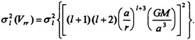
(A16)
A.8 ACCURACY VERSUS RESOLUTION IN GAUSSIAN-WEIGHTED AVERAGES OVER A SPHERICAL CAP
We follow Jekeli (1981) in using a spherical approximation to an isotropic Gaussian convolution filter (weighted average) as follows. Define the weight function
(A17)
where again Ψ is the angular distance between two points on the sphere, and α is a positive constant. The leading constant in (A17) normalizes the weight function so that its integral over the surface of a sphere is one. The parameter α is analogous to the reciprocal of the variance in a Gaussian weight function, for when Ψ is small we have
(A18)
The angle at which the weight function has one half of its maximum amplitude, Ψ½, is
(A19)
and the resolution length appearing on the horizontal axis of many figures in this report is √πR Ψ½ where R is the mean radius of the Earth. This resolution length is the side of a square having the same area as a spherical cap of radius Ψ½
In order to form Gaussian-weighted averages from degree variances, we need the Legendre expansion of the weight function. Define βl by
(A20)
so that
(A21)
Now, to form the resolution accuracy estimate, let be the degree variances of the errors in the spherical harmonic coefficients of the gravity field. These are adjusted, as explained in Chapter 2, so that if the degree variance of the error from a satellite mission exceeds the degree variance of the signal in the
gravity field, the signal in the gravity field is used instead. The root-mean-square accuracy of the Gaussian-averaged geoid height, egeoid, is given by
(A22)
and the root-mean-square accuracy of the Gaussian-averaged gravity anomaly, egravity, is given by
(A23)
where the sums can be safely truncated at a finite limit L that depends on a. We found that, for the range of resolution lengths considered here, L = 1900 was sufficient.


