Research Required to Support Comprehensive Nuclear Test Ban Treaty Monitoring (1997)

Assessment of the seismic monitoring of a CTBT requires working definitions of the threshold level in terms of seismic magnitude, and several discriminants depend on accurate determination of the seismic magnitude (in one or more frequency ranges). For example, one of the most successful and proven teleseismic methods to discriminate seismic events is the classical m_b: M_s comparison, for which explosions have a significantly smaller surface wave magnitude (M_s, measured from the peak long-period surface wave amplitude at a period of about 20 seconds) than an earthquake with the same body wave magnitude (m_b, measured from the peak short-period P-wave amplitude, typically near a period of 0.5–1.0 seconds. The effectiveness of this discriminant is attributable to the difference in the characteristic dimensions of the two sources: an earthquake ruptures over a plane which is large in size relative to the cavity created by an underground explosion. One can also think of this source difference in terms of the time function excitation, which tends to be long for earthquakes and short and impulsive for explosions. Important contributions to this discriminant also come from the inefficient excitation of Rayleigh waves from an isotropic source and the rebound of the explosion cavity which produces a peak in the amplitude spectrum.

Significant challenges have arisen as the monitoring community has attempted to extend this and related teleseismic discrimination methods to smaller events recorded at regional distances: the relative source dimensions change, fewer stations record signals from the events, the paths are more variable and complex, and the complexity introduces differences in numbers and characteristics of the signals (e.g., frequency content and amplitude). These differences require definitions of source magnitude that are (1) consistent with the teleseismic estimates for large events that are recorded both regionally and teleseismically; (2) are applicable in those cases where only regional stations detect signals; and (3) can be normalized from one region to the next. This appendix reviews the nature of seismic magnitudes along with more physically well-defined measures of source strength involving seismic moment and seismic wave energy derived from waveform modeling approaches.

The procedure for assigning magnitudes to seismic sources originated with Richter (1935), who used recordings made on a specific instrument

(the Wood-Anderson) to estimate the relative size of local earthquakes in southern California. He constructed an empirical standard curve that characterized the variation in observed amplitudes (log of the peak amplitude on any component) with distance from an event. This empirical curve was then used to reduce the measurement made at the actual epicentral distance of the seismometer to that expected for a seismometer at 100 km. This magnitude scale is known as M_L and is localized to southern California. Figure D.1 provides examples of the differences in signals from nuclear explosions and earthquakes at the Nevada Test Site (NTS) recorded at a broadband station in Pasadena, California (the signals are filtered to correspond to various classical instruments). The local magnitudes for these two events, averaged over the array of simulated Wood-Andersons from broadband stations in southern California, are M_L = 5.6 for the explosion (Kearsarge: the U.S. joint verification experiment [JVE] explosion) and 5.7 for the Yucca Mountain earthquake. Note that there is an order-of-magnitude larger surface wave for the earthquake compared to the explosion despite their comparable short period amplitudes that result in similar local magnitudes.

One of the most common measures of seismic source strength (m_b) is based on the P-wave amplitude. Essentially, a peak-to-peak amplitude (A) measurement is taken from the first 4 seconds of each record of a short-period vertical component recording or array beam along with an estimate of the period (T) of the peak motion. After A is corrected for the instrument amplification factor at that period, the body wave magnitude is calculated from the average of measurements at j stations: m_b^j = log₁₀ (Aj/Tj) + B(Dj) + Sj (j = 1, …, j). Here B(Dj) is an empirical correction factor for source depth and epicentral distance [conceptually, m_b can be calculated for stations at any distance, as long as the B(Dj) value is established for the particular phase being measured, such as Pn, P, or PKP], and Sj is an empirical station correction factor based on relative station amplitude patterns. Averaging observations is essential, given the large variance in magnitude measurements for a given event (for measurements without station corrections this varies over one full magnitude unit or more, as a result of heterogeneous propagation effects or azimuthal variations in the radiation patterns, and even when station corrections are used, there is a typical scatter of at least 0.3 unit of magnitude). Statistical methods can be used to allow for amplitude measurements that are off-scale or that are below the noise to give the most consistent relative magnitude determinations. As events of interest become smaller, the number of observations that contribute to their magnitude estimation decreases, and the associated uncertainty in magnitude value increases. The development of threshold estimates or discrimination techniques for small events must account for these factors.

Because explosions can be idealized as rapidly occurring isotropic pressure sources, they often produce strong impulsive, relatively simple P waves at teleseismic distances. Thus, one of the earliest methods for estimating explosion yields was based on relating m_b to yield empirically at teleseismic distances. Following the standard m_b versus yield approach (e.g., Dahlman and Israelson, 1977), known events with known yields are used to construct a curve (usually a straight line) relating m_b to yield. When m_b is measured for a new event, the curve is used to estimate the yield corresponding to that m_b.

Given the close cooperation between Russian and U.S. seismologists in past decades, yields are now known at the major test sites, and curves of m_b versus yield are well established for medium size underground explosions. Adushkin (1996) gives m_b (ISC) = 0.86 log W + 3.87 for the Nevada Test Site, and m_b (ISC) = 0.77 log W + 4.45 for the East Kazakhstan test site for well-coupled events with yields less than 150 kt. Note the large difference in m_b for 1 kt yield events: 3.87 versus 4.45. This results from a combination of source coupling and upper-mantle attenuation effects for each test site. The m_b (ISC) values are determined without any station corrections, but rely on relatively large numbers of stations, so data censoring effects are not likely to be too severe except for the largest and smallest events used to determine the above relationships.

Events with m_b < 4 are usually recorded only regionally, and in Adushkin's study these were calibrated against larger events for the same paths by assuming that the entire NTS area is a uniform source region. Thus, the B(D) corrections to m_b,

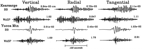
FIGURE D.1 Three-component broadband records for the Kearsarge Joint Verification Experiment at the Nevada Test Site and a Yucca Mountain earthquake near NTS recorded in Pasadena, California. Simulated short-period records for the events (derived from broadband measurements) are indicated as WASP. The amplitudes of the displacements for all records are noted in centimeters. Although there is an order-of-magnitude difference in the amplitude of the broadband data, M_L for the earthquake and the explosion are comparable (5.6 Kearsarge, 5.7 Yucca Mountain.) because of their similar short-period response (WASP). Source: D. Helmberger.

which are poorly constrained at regional distances, become less important since the station corrections for this well-calibrated source area absorb any offset. However, as pointed out by Adushkin (1996), the scatter in M_L (Berkeley) relative to NEIS m_b was -0.2 to +0.7 units for the 14 smallest shots considered, and this high variance is not explained. In general, measurements of m_b using regional phases have high variance.

A magnitude scale based on teleseismic surface waves was described by Gutenberg and Richter (1936) and developed more extensively by Gutenberg (1945). It used the amplitude of maximum horizontal ground displacement due to surface waves with periods around 20 seconds and is called

M_s. This scale was generalized by Bath (1967) to

where A is the peak-to-peak amplitude of the Rayleigh wave (amplitude measured in millimicrons on the vertical component) and D is epicentral distance in degrees.

The U.S. Geological Survey (USGS) NEIS uses this formula, but restricts measurement to the period range 18 < T < 22 seconds, and thus explicitly avoids regional Rayleigh waves (Airy phase) such as those displayed in Figure D.1, which have shorter predominant periods. The requirement of measurable 20-second-period Rayleigh wave arrivals is quite demanding for small events, particularly for isolated seismometers. As a result, conventional M_S is effectively restricted to events with m_b > 4.0–4.5. However, since the Rayleigh waves at Pasadena (PAS) for the NTS Kearsarge explosion look quite similar to those for lower-yield events (Woods et al., 1995), it appears viable to estimate M_S at all ranges if a stable correction for the signal period is made. This proves difficult because the strength of the regional Rayleigh waves depends on many factors: source type, source depth, local structure, and attenuation.

The approach taken for extending M_S to regional distances by Woods and Harkrider (1995) involves modeling the Rayleigh waves produced by NTS explosions at all distances by assuming a mixed path correction, essentially a local structure at NTS and a regional structure along the path to the station obtained from prior efforts of Stevens et al. (1982). The formalism of

Levshin (1985) is used, which treats the propagation of Rayleigh waves along a slowly varying inhomogeneous path as developed earlier by Woodhouse (1974). These approximations are used routinely in the Harvard Centroid-Moment Tensor (CMT) solutions. The Woods and Harkrider (1995) study determined an effective long-period seismic moment M ₀ first and then determines an equivalent teleseismic M_s. They report on 50 North American stations observing 190 NTS explosions where the regional events are on-scale for small events and not observed at some of the more distant stations. They obtain M_s = log M₀ + b, where b = 11.38 for NTS.

A similar study by Stevens for the Semipalatinsk, East Kazakhstan, test site involving primarily teleseismic data obtained b = 11.86. Thus, NTS appears less effective in producing surface wave amplitudes per unit of source strength M₀ or yield than does the Soviet test site. However, the difference in frequency content between explosions and earthquakes implied by the East Kazakhstan experiment suggests that m_b:M_s discriminants should be even more effective in central Eurasia than in the western United States.

Given the difficulties of estimating m_b from Pn for small events and recognizing that Lg signals are typically larger than Pn signals, Nuttli (1973) introduced the Lg magnitude scale m_b (Lg). The short-period Lg phase defined by Nuttli has an apparent velocity of about 3.5 km/s. The phase generally looks slightly dispersed in character as seen in Figure D.1 (Lg arrives about a minute after the first arrivals [Pn] in these observations). Nuttli assumed the Lg arrival to be formed from the superposition of higher-mode surface waves, and because superposition combines energy leaving the source at many different angles, it should require fewer measurements at fewer stations than m_b to suppress radiation pattern effects (Dainty, 1996). Nuttli picked the third largest amplitude in the window formed by velocities 3.2 to 3.6 km/s as representative of strength and reduced the measurement to a distance of 10 km similar to Richter's local magnitude approach. He defined m_b(Lg) = 5 + log₁₀ [A(10 km)/110], where A is measured in millimeters and corrected for attenuation by assuming a decay of A proportional to exp[-a (D × 10)] (see Douglas and Marshall, 1996, for a discussion).

The attenuation parameter a is estimated from the actual record directly, as discussed by Herrman (1980). Nuttli (1985) showed that NTS yields can be estimated remarkably well by applying this methodology to a few regional stations. The procedure has been repeated by Patton (1988) using some changes in definitions and yielded similar results. Thus, if a path can be calibrated well, this measure proves highly stable compared to m_b (Pn). Unfortunately, Lg is subject to path blockage caused by complexity in crustal structure in some regions.

Stable single-station estimates of magnitude made using the envelope of the 1 Hz Lg coda show promise for regional seismic monitoring (Mayeda, 1993). The Lg coda is generated by scattering, but decay of the Lg coda appears to be controlled by anelastic losses. Amplification effects near the recording stations and attenuation control the absolute amplitude, but the decay rate of the coda depends on the average medium properties of the crust sampled by the coda waves. Given limited calibration information from a region, coda magnitudes appear to provide high-precision estimates of magnitude using the data recorded at even one station.

The amplitude of the Lg coda is modeled by the equation:

where A_c(t) is the noise-corrected, time-dependent Lg coda amplitude; N contains both source and receiver effects; t is time in seconds, and a and b are constants representative of the medium from the path to the receiver (a and b are determined by fitting the shape of the curve to the noise-corrected amplitudes for the Lg coda). Given these values, the coda magnitudes are normalized to m_b(Lg) by assuming that log₁₀ (N = m_b(Lg) + constant, where the constant provides the station correction. Once the station correction is determined, the equation can be used to determine an estimate of m_b(Lg) for a new event, given the measurement of A_c(t) for that event.

The explosion monitoring methodology in current use has developed around the magnitude scales described above. Some efforts were conducted by ARPA during the mid-1980s to place yield estimation on a modeling basis, but uncertaintles in how to treat the surface interaction (pP) in the presence of spall, near-field attenuation, tectonic release, and so forth, proved too large to be competitive with the more direct empirical procedures (see Murphy, 1996). Large events, which provide many observations for averaging, allow meaningful comparison of explosion and earthquake sources, but near the monitoring threshold there will be few observations of each event. The assumption of averaging over many stations to remove source and path effects begins to break down when extensive averaging cannot be performed. Operational questions arise for smaller events: for example, should the station magnitude corrections determined by processing teleseismic signals be applied to observations at closer distances; should magnitude corrections be derived by systematically correcting for biasing effects of earthquake source orientation as suggested by Pearce (1996)?

An alternative to the empirical approach of estimating source strengths involves waveform modeling methodologies. Examples of routine earthquake processing with such approaches include Harvard's solutions for long-period body and surface waves (Dziewonski et al., 1981) and USGS moment tensors from teleseismic P waves (Sipkin, 1982). The former method uses a three-dimensional Earth model and locates the event as it finds the optimal source representation. The latter method relies on the NEIS location. Both approaches can provide globally complete focal mechanism solutions for events above m_b = 5.0–5.5, but various strategies allow similar routine source inversions to be made for smaller events using regional signals (e.g., Ritsema and Lay, 1993).

New analytical tools have been developed recently to estimate source parameters from broadband regional seismic data. Two kinds of regional waveform data are typically used for source estimation: surface waves (e.g., Patton, 1980; Patton and Zandt, 1991; Thio and Kanamori, 1995) and body waves (e.g. Wallace and Helmberger, 1982; Fan and Wallace, 1991; Fan et al., 1994; Dreger and Helmberger, 1993). Generally, body waves are less affected by shallow heterogeneities and are more stable than surface waves, although they have a lower signal-to-noise ratio due to their lower energy. There have been several inversion methods proposed recently using whole seismograms (Ritsema and Lay, 1993; Walter, 1993; Zhao and Helmberger, 1994; Nabelek and Xia, 1995). Most of these inversions are controlled mainly by surface waves, particularly because they are performed using long-period waveforms.

An exception is the "cut-and-paste" (CAP) method of Zhao and Helmberger (1994), which breaks broadband waveforms into Pnl and surface wave segments and inverts them independently. The source mechanism is obtained by applying a direct grid search through all possible solutions to find the global minimum of misfit between the observations and synthetics, allowing time shifts between portions of seismograms and synthetics to reduce the influence of poorly known structure. One advantage of the technique is that it proves insensitive to velocity models and lateral crustal variation. Source resolvability as a function of stations and components is discussed in Zhao and Helmberger (1994). Song et al. (1996) performed a detailed sensitivity study and showed that a single two-layered crustal model produces an adequate set of synthetics to fit most earthquakes in the western United States if time shifts are allowed. More detailed modeling may provide better fits and less shifting but has little effect on the resulting source parameter estimates. The inversion discussed above has been further stabilized by including absolute amplitudes and is fully automated on the TERRAscope data stream in southern California (Zhu and Helmberger, 1996).

Various comparisons of long-period surface wave magnitude (M_s or M₀) levels can be made

with short-period body waves [m_b, m_b(Pn), M_L] to assess characteristic spectral behavior of different source types. Of particular importance is the behavior seen at regional distances. A plot of M_L versus M₀ for a population of NTS explosions and western U.S. earthquakes is given in Figure D.2. The type of source was assumed to be known in determining M₀ values, so this is not a discrimination plot, but an indication of physical differences between the sources.

There is a significant separation of earthquake and explosions using this criterion, with no real overlap of the two populations although several earthquakes plot near the explosion region. This separation exists at all sizes. It appears that explosions and earthquakes follow separate respective scaling laws over a wide range of local magnitudes and moments. For earthquakes there is relatively simple scaling over seven and a half orders of magnitude. Earthquakes with a log moment below 13.0 nm were determined from local stations (D < 1¹) and would not be detectable at larger distances. They are included here to show the continuity of the linear scaling relationship between M_L and log M₀ for earthquakes.

There is significant scatter in both data sets. The amount of stress relieved by an earthquake is a function of the material properties of the source region and the shape of the surface over which the fault ruptures. Higher-stress drop events are richer in high-frequency energy; thus, the ratio of short-to long-period magnitude fluctuates somewhat from one earthquake to the next. The spectral signature of explosions is also known to depend on the emplacement medium. Explosions can also release ambient stress within the Earth's crust. This tectonic release creates a secondary seismic source that can modify the energy radiation pattern as well as the spectral character of the source. These effects can vary the short-to long-period magnitude ratio of explosions.

These differences of source spectra are quite similar to those presented by Patton and Walter (1993) for the well-calibrated region around the

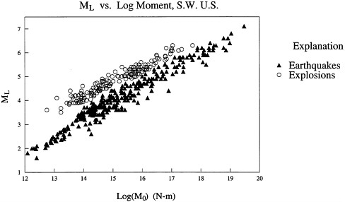
FIGURE D.2 Local magnitude versus event seismic moment (M₀) for earthquakes and explosions in the Southwestern United States. Source: D. Helmberger.

NTS in terms of m_b(Pn):M₀ and m_b(Lg):M₀ and the results presented earlier by Taylor et al. (1989) on regional m_b(m7.9):M_s. Some regional discriminants are designed to detect these source differences.

The initial stages of underground explosion monitoring were driven almost entirely by empirical relationships involving these magnitudes. It was noted 30 years ago that P waves from underground shots become quite simple at distance ranges beyond 30¹ (3300 km) and that the existing m_b (teleseismic body wave magnitude as introduced by Beno Gutenberg) was a convenient indicator of source strength. Consequently, m_b-yield relationships have been used to estimate yields globally with a long and ultimately successful history (Schlittenhardt, 1988) involving an instructive interplay between policy and technology. Similarly, surface wave magnitudes at teleseismic distances M_s were used to establish empirical M_s-yeild relationships. For well-coupled explosions in a tectonically active area such as NTS, the empirical relationship

where m_b is determined teleseismically from a large number of stations and W is yield in kilotons, proves quite effective (Murphy, 1996). Offsets in the regression line became obvious when comparing NTS data to those for explosions at the Amchitka test site (e.g., von Seggern and Blandford, 1972). Distinct differences in plots of m_b versus M_s for U.S. and Soviet tests were also easily recognized (e.g., Bache, 1982). These features were resolved after considerable scientific and policy debate by allowing for differences in upper-mantle attenuation levels. For example, yield estimates based on m_b for well-coupled underground explosions at the Semipalatinsk test site are well matched by

The m_b values are adjusted upward relative to NTS because of lower attenuation in the mantle under this site (e.g., Murphy, 1996). The two relationships given above were derived before their validation by JVE tests, which is considered to be one of the triumphs of the U.S. research and monitoring community.

Theoretical source models that have been developed to match observed seismic signals, such as the Mueller-Murphy model, prove quite effective at predicting teleseismic P-wave amplitudes in diverse media. For example, the m_b generated by events in clay-or water-filled cavities can be 0.5 magnitude units higher (factor of 3 greater amplitudes) than for normal hard rock sites, whereas a reduction of 0.5 unit is expected for events in dry porous media (Murphy, 1996).

Although spherical source models for explosions work well for explaining P waves, they do poorly in predicting the remaining portions of seismograms, especially at regional distances where measures of ML and Lg are made. The difficulty is that these observations are usually controlled by shear waves (see Figure D.1), which in principle are not excited by an explosion source. Shear wave excitation by explosions is partly explained by triggered tectonic release, but this is difficult to predict, especially in remote regions with no testing history. Tectonic release does appear to produce scatter in M_s for some test sites, which has made mb the more attractive measure of yield.

Much of the source strength research conducted by the seismic monitoring community has addressed events with yields greater than 100 kt relevant to the Threshold Test Ban Treaty (TTBT). These events have m_b values near 6 and are well recorded globally, typically with more than 30 stations reporting magnitude values at teleseismic distances where the paths travel deep in the Earth and avoid upper-mantle complexity. Although individual distance-corrected P-wave amplitudes at these ranges can vary by factors of 10, the network average magnitude tends to be quite stable when large numbers of observations are available. Station corrections and source region biases established empirically for large events can be applied to smaller events located near the larger ones as long as signals are detectable at the same stations. For yields of 1 kt, which have seismic magnitudes near 4.0, only a few teleseismic observations are usually available. This requires use of regional data to estimate mb. At regional

distances, amplitude-distance curves become highly variable, and they are unknown in the regions where many of the new IMS stations are being installed.

At regional distances it is possible to use empirical magnitude measures and to define station corrections similar to those at teleseismic ranges. However, regional distance signals have more complex propagation effects, and as a result, source strength estimation may be better performed by quantitative modeling procedures that synthesize complete seismic signals, explicitly accounting for propagation complexities, or use features such as the coda of the wave, which are less dependent on specific paths. Modern instrumentation, coupled with recent modeling techniques, allow complete long-period (>30-second) regional signals to be modeled down to magnitude 4.5–5.0 with simple velocity models (Ritsema and Lay, 1993), whereas shorter-period data (down to 5-second period) can be modeled for events as small as magnitude 3.5 in regions with well-determined velocity structures such as California (Zhu and Helmberger, 1996).