
E— Description of Age-Structured Simulation Model
Jie Zheng and Terry Quinn*
Each of the five data sets contains statistics from the fishery: reported catch, effort, and age composition. Survey data are summarized as a relative index along with survey age composition. Simulations were initiated in year -15 in a pristine population condition and ended in year 30. Fishery and survey data from years 1 to 30 were given to the analysts for stock assessment analyses. The population contains ages 1 to 15, where age 15 represents fish of 15 years age and older, although fish older than 15 are uncommon. Parameters are summarized in Tables E.1 and E.2.
In the description below, a denotes age and t denotes time. The age-structured model used to create simulated data sets has the following features:
- Natural Mortality Mt: This is a random variable drawn as an annual value from a uniform distribution ranging from 0.18 to 0.27; the natural mortality is constant over age.
- Growth: Mean weight at age follows an isometric von Bertalanffy curve
where W![]() = 5000 g, k = 0.3 per year, β1 = 3, and t0 = year 0.
= 5000 g, k = 0.3 per year, β1 = 3, and t0 = year 0.
|
3. |
Maturity: The maturity relationship is a logistic-shaped function The bm parameter is constant over the five data sets and equal to 1.65 per year. The am parameter is the age at 50% maturity and varies among data sets. Both the growth and the maturity relationships are based on true age. |
|
4. |
Spawner-Recruit Model: Spawning (S) is assumed to take place at the start of the year. Recruitment (R) is |
|
* |
Jie Zheng and Terry Quinn constructed the Excel model using committee specifications and created the simulated data sets using the Excel model. |
TABLE E.1 Summary of Simulated Population Parameters for the Five Data Sets
|
Parameter |
Data Set 1 |
Data Set 2 |
Data Set 3 |
Data Set 4 |
Data Set 5 |
|
Mt |
0.18-0.27 |
0.18-0.27 |
0.18-0.27 |
0.18-0.27 |
0.18-0.27 |
|
W |
5000 |
5000 |
5000 |
5000 |
5000 |
|
k |
0.3 |
0.3 |
0.3 |
0.3 |
0.3 |
|
β1 |
3 |
3 |
3 |
3 |
3 |
|
t0 |
0 |
0 |
0 |
0 |
0 |
|
am |
7 |
8 |
9 |
8 |
7 |
|
bm |
1.65 |
1.65 |
1.65 |
1.65 |
1.65 |
|
α |
3.8742 |
4.8276 |
6.1711 |
4.8276 |
3.8742 |
|
β |
4.54 × 10⁻³ |
4.53 × 10⁻³ |
4.82 × 10⁻³ |
3.23 × 10⁻³ |
2.27 × 10⁻³ |
|
σ |
0.6 |
1.0 |
0.9 |
0.7 |
0.8 |
|
ρ |
0.5 |
0.5 |
0.5 |
0.5 |
0.5 |
|
R0 |
800 |
1000 |
1200 |
1400 |
1600 |
|
Σ10 |
-1.0 |
-1.0 |
-1.0 |
-1.0 |
1.0 |
|
af (t = -15 to 20) |
5 |
5 |
5 |
5 |
5 |
|
bf (t = -15 to 20) |
0.8 |
0.8 |
0.8 |
0.8 |
0.8 |
|
af (t = 21 to 30) |
5 to 3 |
5 to 3 |
5 to 3 |
5 |
5 |
|
bf (t = 21 to 30) |
1.0 |
1.0 |
1.0 |
0.8 |
0.8 |
|
σf |
0.2 |
0.2 |
0.2 |
0.2 |
0.2 |
|
q0 |
0.01 |
0.01 |
0.01 |
0.01 |
0.01 |
|
q1 |
0.4 |
0.4 |
0.4 |
0.4 |
0.4 |
|
σq |
0.2 |
0.2 |
0.2 |
0.2 |
0.2 |
|
r (t = -15 to 0) |
0.0 |
0.0 |
0.0 |
0.0 |
0.0 |
|
r (t = 1 to 30) |
0.0135 |
0.0135 |
0.0135 |
0.0135 |
0.0135 |
|
E0 |
2738.2 |
2849.4 |
2922.8 |
3486.8 |
4150.3 |
|
E1 (t = -14 to 1) |
0.5 |
0.2 |
0.4 |
0.4 |
1.7 |
|
E1 (t = 2 to 30) |
0.68 |
0.65 |
0.8 |
0.8 |
0.3 |
|
Underreporting |
0% |
30% |
0% |
0% |
0% |
|
α' |
3.2322 |
3.2322 |
3.2322 |
3.2322 |
3.2322 |
|
β' |
3.3382 |
3.3382 |
3.3382 |
3.3382 |
3.3382 |
|
q*0 (t = 1 to 15) |
2.0 × 10⁻⁶ |
2.0 × 10⁻⁶ |
2.0 × 10⁻⁶ |
2.0 × 10⁻⁶ |
2.0 × 10⁻⁶ |
|
q*0 (t = 16 to 30) |
2.0 × 10⁻⁶ |
2.0 × 10⁻⁶ |
4.0 × 10⁻⁶ |
2.0 × 10⁻⁶ |
2.0 × 10⁻⁶ |
|
σ* |
0.3 |
0.3 |
0.3 |
0.3 |
0.3 |
- defined as abundance at age 1; thus, Rt = N1,t. Recruitment is assumed to follow a Beverton-Holt model with autocorrelated errors:
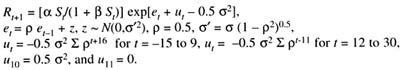
The error ε10 was set to be negative (-1) for declining data sets 1-4 and to be positive (1) for data set 5 (recovering
TABLE E.2 Summary of Reference Fishing Mortality and Effort and Associated Exploitable Biomass and Yield for the Five Data Sets
|
Parameter |
Data Set 1 |
Data Set 2 |
Data Set 3 |
Data Set 4 |
Data Set 5 |
|
F40% |
0.131 |
0.119 |
0.109 |
0.158 |
0.182 |
|
E40% |
980.14 |
817.08 |
914.46 |
1405.12 |
1598.84 |
|
B40% |
2596.32 |
2269.25 |
3183.21 |
3466.97 |
3416.25 |
|
Y40% |
289.22 |
229.61 |
295.45 |
464.35 |
521.31 |
|
FMSY |
0.196 |
0.158 |
0.151 |
0.252 |
0.280 |
|
EMSY |
1222.8 |
949.1 |
1096.37 |
1826.68 |
2024.99 |
|
BMSY |
1924.38 |
1819.5 |
2479.86 |
2476.98 |
2473.06 |
|
MSY |
312.20 |
240.46 |
315.18 |
512.68 |
563.53 |
|
FMSY1 |
0.297 |
0.225 |
0.208 |
0.252 |
0.280 |
|
EMSY1 |
2302.01 |
1722.76 |
1939.33 |
2740.02 |
3037.49 |
|
BMSY1 |
1410.40 |
1379.94 |
1911.31 |
2476.98 |
2473.06 |
|
MSY1 |
339.53 |
257.13 |
331.41 |
512.68 |
563.53 |
- stock) to force recruitment to be low for data sets 1-4 and high for data set 5. The above adjustments were done so that the expected value of recruitment follows the deterministic Beverton-Holt curve. Note that α and ut can be combined as αt = α exp(ut).
Parameters σ, α, β and R0 (pristine, initial recruitment in millions) vary among data sets.
- Population Abundance and Mortality Equations:
Abundance
Total mortality

Fishing mortality

where sa is selectivity, qt is catchability, and Et is fishing effort for the commercial fishery, described further below.
- Catch Equation: Fishing and natural mortality occur continuously throughout the year, so that catch (C) follows from the Baranov equation:

The catch for age 1 was small and reported as none.
|
7. |
Yield and Biomass: Yield (Y, catch in weight) and biomass (B, population size in weight) are obtained by multiplying catch and abundance (in numbers of fish) by average weight: |
|
8. |
Fishery Selectivity: One fishing gear was assumed for the simulation and the selectivity (S) for the fleet is a logistic function |
- For data sets 1-3,
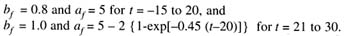
For data sets 4-5,
For all data sets, af is equal to its expected value plus a value randomly between -1 and 1.
|
9. |
Fishery Catchability: Catchability (q) was assumed to have a exponential time trend and an allometric dependence on biomass: for all data sets, where q0 = 0.01, q1 = 0.4, and t0 = 0. Parameter r = 0 and Bt = B |
|
10. |
Fishing Effort: Et = E0E1v, where v ranges from 0.75 to 1.25 randomly for all data sets, E0 is a constant fishing effort, and E1 is a constant. Both E0 and E1 were adjusted for different data sets to get desirable abundance trends over time. Reported effort is the true effort for all data sets. |
|
11. |
Reported Catch: Total reported catch equals (true catch) × (1 - underreporting %) × u, where u ranges from 0.97 to 1.03 randomly each year. Underreported total catch and total yield are 30% for data set 2 and 0% for all other data sets. Reported yield in biomass is determined from landing reports, not as the sum of catch-age times weight-age. Reported catch in numbers is also not affected by age composition. |
|
12. |
Survey Abundance: The survey occurs during a short period of time at the beginning of each year immediately after spawning, after recruitment, and before any mortality occurs. We follow the convention that birthdate is assigned at the beginning of each year just prior to spawning. The survey abundance index is calculated as |
|
13. |
Survey Selectivity: The selectivity for the survey gear is a gamma function where α' = 3.2322 and β' = 3.3382, resulting in s*3 = s*15 = 0.5 and *s7 = 1.0. |
|
14. |
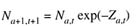
Survey Catchability: The survey catchability is a constant multiplied by a random variable: where q*0 = 0.000002 for t = 1 to 30, except for data set 3 for which q*0 = 0.000002 for t = 1 to 15 and q*0 = 0.000004 for t = 16 to 30. |
|
15. |
Sample Size for Age Composition: Simple random samples of age composition were taken from the catch (n = 500) and from the survey (n = 200). |
|
16. |
Ageing Error: Ageing error is the difference between the age reader's estimated age of a fish and its true |
- age. We assumed that a single reader aged all fish. Ageing error was generated with 0 bias at age 1, which increases linearly to -1 at age 15. The variation in ageing error was ~N(0,
 2), with a linear increase in standard deviation from = 0 for age 1 and = 2 for age 15. This resulted in a misclassification matrix (the age error matrix was provided to the analysts) whose elements are the probabilities pi,a that an individual of true age i is estimated to be age a.
 - Reference Fishing Mortality and Effort: Under the expected fishery selectivity and catchability in year 30, full-recruitment fishing mortality (F40%) and effort (E40%) in boat-days that reduce spawning biomass per recruit to 40% of the unfished level as well as the associated expected exploitable biomass (B40%) and yield (Y40%) in thousand metric tons, are given in Table E.2. Under the deterministic condition, full-recruitment fishing mortality (FMSY) and effort (EMSY) in boat-days at MSY (maximum sustainable yield), as well as the associated expected exploitable biomass (BMSY) and MSY in thousand metric tons are also given in Table E.2.
Full-recruitment fishing mortality (FMSY1) and effort (EMSY1) in boat-days at MSY and the associated expected exploitable biomass (BMSY1) and MSY in thousand metric tons were determined using the expected fishery selectivity and catchability in year 1 and deterministic conditions.


