Improving Fish Stock Assessments (1998)

Assessment methods generally are based on two types of mathematical models: (1) a model of the dynamics of the fish population under consideration, coupled with (2) a model of the relationship of observations to actual attributes of the entire fish population. These models are placed in a statistical framework for estimation of abundance and associated parameters and include assumptions about the kinds of errors that occur in each model and an assumption about the objective function* used to choose among alternative parameter values. These errors can be characterized broadly as either process errors or observational errors.

Process errors arise when a deterministic component of a population model inadequately describes population processes. Such errors can be found in the modeled relationships between recruitment (or year-class abundance) and parental spawning biomass and can occur as unpredictable variations in the age-specific fishing mortality rates of an exploited population from year to year. In contrast, observational errors arise in the process of obtaining samples from a fishery or by independent surveys. Decisions must be made regarding the type of probability distribution appropriate for each kind of error (e.g., normal, lognormal, or multinomial) and whether errors are statistically independent, correlated, or auto-correlated.

The form of the objective function chosen for parameter estimation is based on a likelihood function.† In the models reviewed in this report, the objective is to maximize the total log-likelihood function. The total log-likelihood is generally a weighted sum of log-likelihood functions corresponding to the different types of observations. It is often simplified to an analogous problem of minimization of weighted least squares.

This report concentrates on complex population models, although the committee acknowledges that less structured stock assessment approaches may be more appropriate for some fisheries, as described in Chapter 1. Examples include the use of linear regression models for some Pacific salmon species and multispecies trend analyses (Saila, 1993).

General types of population models include surplus production, delay-difference, age-based, and length-based models (see Chapter 5 for specific references and more detailed descriptions of the models used in this study). They rely on rates of change in biomass and productivity that can be calculated based on information about yield from fisheries, recruitment, and natural deaths. Detailed presentations of these models are given in Ricker (1975), Getz and Haight (1989), Hilborn and Walters (1992), and Quinn and Deriso (in press). Models of population change can be written as a differential equation

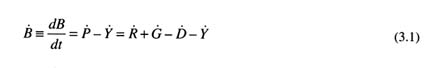
or, in words, the rate of change in biomass () equals productivity () minus yield (). The productivity of a population depends on the recruitment of progeny () and the growth () and death () of existing individuals. Barring time-dependent processes in Equation (3.1), equilibrium biomass and yield result only if some of the rates in Equation (3.1) are regulated by population densities; otherwise, the population can either increase or decrease without limit.

This type of model can be implemented with an instantaneous response (no lags) or 1-year difference equation approximation. These models have simple productivity parameters embedded and require no age or length data (Schaefer, 1954; Fletcher, 1978; Prager, 1994). Estimation is accomplished by fitting nonlinear model predictions of exploitable biomass to some indices of exploitable population abundance (usually standardized catch per unit effort, CPUE). The primary advantages of surplus production models are that (1) model parameters can be estimated with simple statistics on aggregate abundance and (2) the models provide a simple response between changes in abundance and changes in productivity. The primary disadvantages of such models are that (1) they lack biological realism (i.e., they require that fishing have an effect on the population within 1 year) and (2) they cannot make use of age- or size-specific information available from many fisheries. However, in some circumstances, surplus production models may provide better answers than age-structured models (Ludwig and Walters, 1985, 1989).

These models incorporate age structure and provide a method for fitting an age- or size-structured population model to data aggregated by age (Deriso, 1980; Schnute, 1985; Horbowy, 1992). Estimation can be accomplished by fitting nonlinear model predictions of aggregate quantities to CPUE, biomass indices, and/or recruitment indices. Delay-difference models are a special-case solution to a more general aggregate-matrix model made possible by the assumption of a particular age-specific growth model (the von Bertalanffy equation [Ricker, 1975]). These types of models share the advantages of surplus production models; additionally, the functional relationship between productivity and abundance accounts for both yield-per-recruit and recruit-spawner effects. Unlike production models, the parameters of delay-difference or aggregate-matrix models have direct biological interpretations, but they cannot make full use of age- or size-specific information. In addition, these models require the estimation of more initial conditions than production models, unless a simplifying assumption, such as an initial equilibrium condition, is made.

Age-based models use recursion equations to determine abundance of year classes as a function of several parameters (Fournier and Archibald, 1982; Deriso et al., 1985; Megrey, 1989; Methot, 1989, 1990; Gavaris, 1993). Relationships between spawning stock biomass and recruitment are not required but can be used. Because of the

flexible nature of such general models, integration of many aspects of the data collection process with the population model is feasible. Estimation can be accomplished by maximum likelihood or least-squares procedures applied to age-specific indices of abundance, age-specific catch, and other types of auxiliary information. The main advantage of these models is that they make almost full use of available age-specific information. The primary disadvantage is that such models require many observations and include many parameters, increasing the cost of using them. ADAPT, Stock Synthesis, and CAGEAN/Cansar* belong in this category. ADAPT is an age-structured assessment method based on least-squares comparison of observed catch rates (generally age specific) and those predicted by a tunable† virtual population analysis. Stock Synthesis is an age-structured assessment technique based on maximum likelihood methods, but with more flexibility to include auxiliary information and fitting criteria. Additional details about ADAPT and Stock Synthesis are provided in Chapter 5.

Models that integrate length and age data are more complicated than age-based models because growth must be specified to relate length to age (Fournier and Doonan, 1987; Schnute, 1987; Deriso and Parma, 1988; Methot, 1990; Sullivan, 1992). This specification is accomplished with a stochastic-growth or length-age matrix conversion. Age structure of these models can be either implicitly or explicitly represented. Because of the flexible nature of such general models, full integration of the data collection process with the population model is feasible. Estimation can be accomplished by maximum likelihood procedures applied to age- and size-specific indices of abundance, age- and size-specific catch, and other types of auxiliary information. The main advantage of this type of model is that it makes full use of both age- and size-specific information. The primary disadvantage is that such models may require many observations and include many parameters.

In terms of data demands and number of parameters, these methods rank as follows (from least to most intensive): production models -> delay-difference models -> size-based models -> age-based (or integrated) models -> length- and age-based (or fully integrated) models. As models become more data intense and complex, there is a decreasing chance of gross model misidentification, an increasing chance of misidentifying some model component, increasing biological realism, and increasing cost of data collection.

Any stock assessment model involves choices at two levels: (1) the structural model that will be used and (2) the parameter values to be used. The choice of models is usually based on past experience. For example, models that assume the stock is in equilibrium are now almost universally avoided because experience has indicated that this assumption is rarely true; equilibrium models tend to produce results that are biased toward optimistic assessments of a stock's productivity. Any model used in an assessment includes many parameters that are assigned based on data other than those used in the assessment. The following are some examples of such parameters:

1. Natural mortality rate is usually assigned a fixed value based on a relationship to maximum age of the species, growth rate, maximum size, or other demographic or life history information (Vetter, 1988).
2. The relationship between indices of abundance and true abundance is generally assumed to be linear (as explained in Chapters 2 and this chapter), and the slope is usually estimated as part of the stock assessment.
3. Recruitment variability is most commonly left unconstrained, but it may be constrained to some value estimated from other data or based on experience.
4. A specific functional form for the relationship between stock and recruitment may be chosen and its

4. parameters estimated jointly with abundance. Other sources of information about stock recruitment parameters can be included in the analysis, although this is not generally done.
5. Depensation* usually is assumed not to occur. Many assessment methods require no specification of this parameter.

If properly calibrated, fishery-independent trawl surveys can be used to estimate the absolute abundance of a fish population. Numbers at age a in year t (N_a,t) can be estimated as

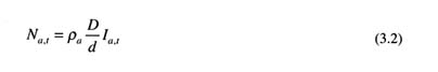
where ρ_a is the probability that a fish of age a in the path of the trawl is captured, D is the area of the survey stratum, d is the area swept by the trawl gear, and I_a,t is the survey index of numbers at age.

For fixed-gear recovery methods (e.g., longlines, pots, gillnets) it is not possible to estimate the area sampled, and even for trawl surveys it is difficult to estimate the probability of capture (ρ_a) accurately. In these cases, estimates from the survey data are assumed to measure relative abundance and are combined with other information about the fish population to estimate existing and past population sizes. In the ADAPT model's original form, the survey estimate of population numbers at age is assumed to be related to actual population numbers as

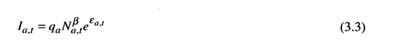
The parameter β is not defined in the model document, but is a commonly used form to express a nonlinear relationship between true abundance and a survey index; q_a represents the catchability of fish of age a to the survey gear and is assumed to be constant over time. The random component of the model (Σ_{a, t}) is assumed to be an independent, symmetrically distributed random variable with constant variance and a mean value of zero. This distributional assumption allows for the use of standard nonlinear least squares to estimate the model parameters (Gavaris, 1993). Recently, Myers and Cadigan (1995) developed a random-effects mixed model within a maximum likelihood framework to estimate the parameters of the ADAPT model. Their approach allows for a correlated within-year error structure for the survey data to deal with "year effects" in survey abundance-at-age estimates (see Smith and Page, 1996). The implicit parameters of Equation (3.3) that must be estimated, whatever the approach, are the fishing mortalities used to estimate N_a in the underlying VPA (virtual population, or cohort, analysis) of the ADAPT method from catch-at-age data (Mohn and Cook, 1993). Absolute abundance is sometimes derived by calculating the area swept by the gear and assuming that all animals in the path of the gear will be captured (i.e., the catchability equals 1). In reality, absolute abundance estimates may be under- or overestimates, depending on whether catchability is greater than 1 due to herding by the trawl gear or less than 1 because of escapement from the path of the trawl.

A different formulation is used in the Stock Synthesis method (Methot, 1990), which more naturally accommodates year effects in the surveys. Instead of fitting the model to age-specific abundance indices, the Stock Synthesis model treats the indices of overall stock abundance separately from the age composition of the survey catches. Thus, year effects affect only year-specific abundance indices and do not introduce correlations among the age-specific observations. The expected value for survey numbers in year t (I_t) for the Stock Synthesis model (Methot, 1990) is determined as

where q is catchability for fully-recruited ages, s_a is age specific availability or selectivity, and N_a,t is population abundance in numbers of fish in year t and age a. The survey can measure either relative (q 1) or absolute (q = 1) abundance. Note the correspondence with the ADAPT formulation in (3.3) by letting q_a = qs_a and β = 1.

In the Stock Synthesis method, variances from the log transform of survey abundance estimates are included, if available, directly in the survey index component of the log-likelihood expression. Therefore, the impact of optimizing the survey design on the resultant estimates from Stock Synthesis can be studied directly. Although there is the possibility of using inverse variance weighting in the nonlinear least squares in ADAPT, this is not usually done. However, bootstrap and Monte Carlo methods are available for linking variation in the survey estimates to variation in the resultant estimates from ADAPT (Restrepo et al., 1992; Smith and Gavaris, 1993b). Ultimately, sampling programs should be evaluated with respect to the precision of the quantities being used to estimate stock status.

The assumption of constant catchability and availability with age over time implied by the use of q_a in ADAPT and s_a in Stock Synthesis can be confounded by changes in both availability and catchability.

Fishery management involves decision-making in the presence of uncertainty. Fishery stock assessments should provide the quantitative support needed for managers to make regulatory decisions in the context of uncertainty. This support includes an evaluation of the consequences of alternative management actions. However, there is often considerable uncertainty that can be expressed as competing hypotheses about the dynamics and state of a fishery. The consequences of management actions may differ depending on which of these hypotheses is true. An appropriate means of providing quantitative support to managers in the presence of uncertainty is through the use of Bayesian statistical analysis. This section discusses the problem of building models of complex fishery systems having many parameters that are unknown or only partially known and the use of Bayesian methodology. Numerous papers and books have been published related to the application of Bayesian analyses in fisheries (e.g., Gelman et al., 1995; Punt and Hilborn, 1997).

There are three major elements in the Bayesian approach to statistics that should be indicated clearly:

1. likelihood of describing the observed data,
2. quantification of prior beliefs about a parameter in the form of a probability distribution and incorporation of these beliefs into the analysis, and
3. inferences about parameters and other unobserved quantities of interest are based exclusively on the probability of those quantities given the observed data and the prior probability distributions.

In a fully Bayesian model, unknown parameters for a system are replaced by known distributions for those parameters observed previously, usually called priors. If there is more than one parameter, each individual distribution, as well as the joint probability distributions, must be described.

A distinction must be made between Bayesian models, which assign distributions to the parameters, and Bayesian methods, which provide point estimates and intervals based on the Bayesian model. The properties of the methods can be assessed from the perspective of the Bayesian model or from the frequentist* perspective. Historically, the "true" Bayesian analyst relied heavily on the use of priors. However, the modern Bayesian has evolved a much more pragmatic view. If parameters can be assigned reasonable priors based on scientific knowledge, these are used (Kass and Wasserman, 1996). Otherwise, "noninformative" or ''reference" priors are

used.* These priors are, in effect, designed to give resulting methods properties that are nearly identical to those of the standard frequentist methods. Thus, the Bayesian model and methodology can simply be routes that lead to good statistical procedures, generally ones with nearly optimal frequentist properties. In fact, Bayesian methods can work well from a frequentist perspective, as long as the priors are reasonably vague about the true state of nature. In addition to providing point estimates with frequentist optimality properties, the posterior intervals for those parameter estimates are, in large data sets, very close to confidence intervals. Part of the modern Bayesian tool kit involves assessing the sensitivity of the conclusions to the priors chosen, to ensure that the exact form of the priors did not have a significant effect in the analysis. There are differences of opinion among scientists about whether frequentist or Bayesian statistics should be used for making inferences from fishery and ecological data (Dennis, 1996).

The basis for selection of the various prior distributions used in a stock assessment should be documented because the choice of priors can be a source of improper use of statistics. A rationale has to be constructed to indicate which models were considered in the analysis and why some models were not considered further (i.e., were given a prior probability of zero), even though they may be plausible. The use of standard procedures permits independent scientific review bodies to verify the plausibility of hypotheses included in the assessment and assign their own prior probability values to the selected hypotheses.

There are two general classes of Bayesian methods. Both are based on the posterior density, which describes the conditional probabilities of the parameters given the observed data. This is, in effect, a modified version of the models' prior distribution, where the modification updates the prior based on new information provided by the data. In one form of methodology, this posterior distribution is maximized over all parameters to obtain "maximum a posterori" (MAP) estimators. It has the same potential problem as maximum likelihood in that it may require maximization of a high-dimension function that has multiple local maxima. The second class of methods generates point estimators for the parameters by finding their expectations under the posterior density. In this class, the problem of high-dimension maximization is replaced with the problem of high-dimension integration.

Over the past 10 years, Bayesian approaches have incorporated improved computational methods. Formerly, the process of averaging over the posterior distribution was carried out by traditional methods of numerical integration, which became dramatically more difficult as the number of different parameters in the model increased. In the modern approach, the necessary mean values are calculated by simulation using a variety of computational devices related more to statistics than to traditional numerical methods. Although this can greatly increase the efficiency of multiparameter calculations, the model priors must be specified with structures that make the simulation approach feasible.

Although they are not dealt with extensively here, a number of classes of models and methods have an intermediate character. For example, there are "empirical Bayes" methods, in which some of the parameters are viewed as arising from a distribution that is not completely known but rather known up to several parameters. There are also "penalized likelihood methods," in which the likelihood is maximized after addition of a term that avoids undesirable solutions by assigning large penalty values to unfeasible parameter values. The net effect is much like having a prior that assigns greater weight to more reasonable solutions, then maximizes the resulting posterior. Another methodology used to handle many nuisance parameters is the "integrated" likelihood, in which priors are assigned to some of the parameters to integrate them out while the others are treated as unknown. This provides a natural hybrid modeling method that could have fishery applications.

A number of features of Bayesian modeling make it particularly useful for fish stock assessments:

1. In a complex model, if a key parameter is treated as totally unknown, the set of parameters of the model

1. may become nonidentifiable (i.e., parameters cannot be estimated consistently no matter how many data are collected). On the other hand, treating a parameter as completely known is too optimistic. Assigning the parameter a known distribution can provide a compromise of including the uncertainty about its true value while retaining the identifiability of the remaining parameters. For example, the natural mortality rate is required in most fishery models but can seldom be estimated accurately. Instead of assuming a known value, natural mortality could be included as a distribution.
2. Fish stock assessment takes place in an environment of decision-making. It involves evaluating possible consequences of alternative actions across competing hypotheses about the system state and its dynamics. Bayesian models are appropriate because they provide probabilities that each of these hypotheses is true, conditional on available information. A distinction can be made between statistical methods designed to provide an estimate based on information in the data alone and those that are designed to use all available information optimally. Bayesian methods allow one to do the latter, following the spirit of National Standard #2 of the Magnuson-Stevens Fishery Conservation and Management Act, which calls for "conservation and management measures … based upon the best scientific information available" (16 U.S.C. 1851).
3. Meta analysis, increasingly used in fisheries science, provides information in an ideal form for Bayesian analysis. For example, if a particular fishery parameter has a distribution over a class of similar species that have been studied more completely, with appropriate adjustment a ready-made prior distribution is available for that parameter in the species of interest.
4. The use of Bayesian models addresses, to some extent, underversus over-parameterization. A model with too few parameters is most likely to provide biased estimators, but with the least variability in its individual estimators. A model with many parameters can fit the actual population dynamics very well but may vary so much over repeated runs that it provides poor estimation. If the larger model has its parameters modeled with informative priors, it lies somewhere between these two options and can be a desirable compromise. A simple model often produces better point estimates merely because the estimates are more stable and less variable, and have some bias that may be insignificant compared to variation. However, a simple model is doomed to underestimate variability. The advantage of a complex model is that all uncertainty is present in the width of the confidence statements rather than hidden.
5. With a completely specified probability model that allows for future uncertainties, simulation studies can provide management strategies that cope with the variability in future fisheries. Forecasting can allow for increasing uncertainty about the future values of input parameters as well as increasing knowledge of the system's fixed parameters.
6. Many complex fishery models are difficult to fit because the likelihood or least squares problems are highly nonlinear. Thus, modeling approaches require the use of multiple starting values and tuning parameters. However, some Bayesian methods are based not on finding maxima or minima but rather on finding posterior means, generally by a process of averaging over separate computer runs. Clearly, this method is more stable as well as more amenable to independent verification, and it is quite repeatable when similar priors are used.

The case for Bayesian methods presented above must be tempered with some limitations of the methods. Several important issues of which the user should be aware include the following:

1. Specification of the priors in a Bayesian model is an emerging art. To do a fully Bayesian analysis in a complex setting, with no reasonable prior distributions available from scientific information, requires a careful construction whose effect on the final analysis is not clear without sensitivity analysis. If some priors are available but not for all parameters, a hybrid methodology, which does not yet fully exist, is preferred.
2. In a complex model, it is known by direct calculation that the Bayesian posterior mean may not be consistent in repeated sampling. However, little information is available to identify circumstances that could lead to bad estimators.
3. Although modern computer methods have revolutionized the use of Bayesian methods, they have created

3. some new problems. One important practical issue for Markov Chain-Monte Carlo methods is construction of the stopping rule for the simulation. This problem has yet to receive a fully satisfactory solution for multimodal distributions. Additionally, if one constructs a Bayesian model with noninformative priors, it is possible that even though there is no Bayesian solution in the sense that a posterior density distribution does not exist, the computer will still generate what appears to be a valid posterior distribution (Hobert and Casella, 1996).
4. There is a relative paucity of techniques and methods both for diagnostics of model fit, which is usually done with residual diagnostics or goodness-of-fit tests, and for making methods more robust to deviations from the model. Formally speaking, a Bayesian model is a closed system of undeniable truth, lacking an exterior viewpoint to make a rational model assessment or to construct estimators that are robust to the model building process. To do so, and retain the Bayesian structure, requires constructing a yet more complex Bayesian model that includes all reasonable alternatives to the model in question, and then assessing the posterior probability of the original model within this setting.
5. Despite the progress in numerical integration of posterior densities, models with large numbers of parameters can be difficult to integrate. Two of the most commonly used methods, (a) sampling importance resampling and (b) Monte Carlo-Markov Chain, each have difficulty with multimodal or highly nonelliptical density surfaces.

Meta analysis is broadly defined as a quantitative method for combining information across related, but independent, studies. The motivation for meta analysis is to integrate information over several studies and to summarize the information. Hedges and Olkin (1985) provide a good explanation of the statistical methods involved. This technique has been applied extensively to biomedical data (D'Agostino and Weintraub, 1995; Marshall et al., 1996) where results from different laboratories and experiments are combined. As applied to stock assessments, meta analysis involves the compilation of preexisting data sets to determine the values of parameters of models or to develop prior probability distributions for these parameters. The most widely used meta analysis method for fisheries was described by Pauly (1980), who examined the relationship among natural mortality rate, water temperature, and growth parameters for a large number of fish stocks. Myers et al. (1994) performed a meta analysis for sensitivity of recruitment to spawning stock, and Myers et al. (1995) conducted a meta analysis of depensation. There are two recent developments in meta analysis for stock assessments: (1) the compilation of large data sets, for example, by Myers and his colleagues; and (2) the application of formal Bayesian methods to estimate prior probability distributions. This allows the use of what is known from other stocks and species to put limits or distributions on parameters and thus obtain a realistic estimate of uncertainty for a new stock or species.

Many parameters are used in stock assessment models, including natural mortality, catchability, potential nonlinearity between indices of abundance, and actual abundance. The general practice has been to assume that some parameters are known perfectly without error. If, however, we were honestly to assess our uncertainty about these parameters, the uncertainty in the overall stock assessment would be large, in some instances, so large as to make results meaningless.

The underlying assumption behind meta analysis is that a parameter is replaced with a random variable. For instance, an estimation of the natural mortality rate among stocks of cod should exhibit a distribution of values. In the absence of any other data for the stock, the distribution from all cod stocks could be used as the probability distribution for the particular cod stock of interest. The distribution among all populations is called the hyper-distribution. The simplest approach to estimating hyper distribution is to plot the frequency distribution of parameter estimates available for all stocks of interest. The problem with such empirical frequency distributions is that each estimate of the parameter for a particular stock involves sampling error. Thus, the empirical distribution is expected to have a higher variance than the true hyper distribution. A method known as hierarchic Bayesian analysis has been developed to deal with this problem and is described in Gelman et al. (1995). This method has been used by Liermann and Hilborn (in press) to develop probability distributions for depensation in spawner-recruit relationships. Eddy et al. (1992) describe a new set of meta analysis techniques known as the confidence profile method, which may be applicable to some fisheries problems.

There are a number of potential problems in meta analysis. Particularly important is the fact that species or

stocks represented in the meta analysis could show patterns of selection bias that would make them unrepresentative (in the variable of interest) within the spectrum of possible species. For example, species of high economic value or large population size are more likely to have been studied in the past, but they could differ in key biological characteristics from the new species of interest.

The reliance of most stock assessment models on time-series data implies not only that each successive assessment characterizes current stock status and other parameters used for management, but also that the complete time series of past abundance estimates is updated. Retrospective analysis is the examination of the consistency among successive estimates of the same parameters obtained as new data are gathered. Either the actual results from historical assessments are used or, to isolate the effects of changes in methodology, the same method is applied repeatedly to segments of the data series to reproduce what would have been obtained annually if the newest method had been used for past assessments.

Retrospective analysis has been applied most commonly to age-structured assessments (Sinclair et al., 1991; Mohn, 1993; Parma, 1993; Anon., 1995b). In such applications, the statistical variance of the abundance (or fishing mortality) estimates tends to decrease with time elapsed; estimates for the last year (those used for setting regulations) are the least reliable. In retrospective analysis, abundance estimates for the final years of each data series can vary substantially among successive updates, whereas those for the early years tend to converge to stable values. In some cases (e.g., some Northwest Atlantic cod stocks, Pacific halibut, North Sea sole), early abundance estimates are consistently biased (either upward or downward) with respect to corresponding estimates obtained in later assessments. Extreme cases of consistent overestimation of stock abundance can have disastrous management consequences, as illustrated by the collapse of the Newfoundland northern cod (Hutchings and Myers, 1994; Walters and Pearse, 1996).

Retrospective biases can arise for many reasons, ranging from bias in the data (e.g., catch misreporting) to different types of model misspecification (mostly parameters that are assumed to be constant in the analysis but actually change, as well as incorrect assumptions about relative vulnerability of age classes). In traditional retrospective analyses, successive assessments use data for different periods, all starting at the same time with one year of data added to each assessment. An alternative method is to conduct successive assessments using data for a moving window of a fixed number of years (as in Parma, 1993, and Deriso et al., 1985). This method is appropriate for exploring trends in parameter estimates.

Ad hoc adjustment factors based on consistent past retrospective errors have been applied occasionally to correct the estimates used for management (e.g., Showell and Bourbonnais, 1994). For example, if past estimates of abundance were shown to be about 40% above the revised estimates obtained subsequently, current estimates could be adjusted downward to compensate, in the expectation that similar bias would also be present in the last year's estimate. Although ad hoc, this may be a sensible precaution in cases of historical overestimation of abundance. Conversely, adjusting current abundance estimates upward to compensate for negative retrospective bias is risky, because the sign of the retrospective errors can reverse without warning; Pacific halibut illustrates such reversal (see Parma and Sullivan, 1996). Adams et al. (1997) have recently developed resampling tests to ensure proper evaluation of the main effects in meta-analysis applications.

Retrospective analysis is an effective tool for uncovering potential problems in an assessment methodology, even if it fails to provide clues about their possible sources. Some of these problems, such as trends in catchability affecting the reliability of the abundance data used for fitting the models, can also be detected as autocorrelation in the residual error terms of statistical analyses. However, the magnitude of the problem is difficult to assess from a single fit to a time series data set. Consistent patterns in retrospective errors indicate problems in the specification of the model; thus, conventional model-based measures of uncertainty of management parameters are not realistic because they are based on the structural assumptions of the model being correct. Because there are many possible sources of the retrospective problem, each specific case has to be considered individually in the search for solutions. An illustration of the use of retrospective analysis is shown in Chapter 5 in a presentation of the committee's analysis of the results of its simulations.

A crucial problem that has emerged in modern stock assessments that combine multiple sources of data and information about population parameters is how to weight each type of information. The typical approach is to define a least-squares or likelihood objective function that contains weight parameters. If {X, Y, …} represent various data sources, X_i is an observation, _i is the corresponding model estimate, and is the variance of that observation, then the typical least-squares objective function is written

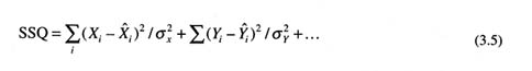
where the data weighting is inversely proportional to variance (Deriso et al., 1985). Similar expressions can be written for likelihood or Bayesian approaches, and this method can be generalized for the situation in which variance changes from observation to observation.

In practice, these variances are unknown, and different approaches have been used to estimate them or to substitute weights {Σ_X, Σ_Y} for the inverse of the variances. Deriso et al. (1985) found that for Pacific halibut data, weighting choice was unimportant for a midrange of weightings. However, many other studies and assessments since then have shown that parameter estimates are related monotonically to the weights chosen. Kimura (1990) showed an empirical approach for obtaining weights from sampling considerations. The variances in Equation (3.5) are often inversely proportional to sample size, suggesting that weighting by sample size is a reasonable approach. Many analysts have no a priori information about weighting, so they assign each observation equal weight. Others prefer to weight each data component equally when the values of different data components differ greatly. Some researchers suggest using perceptions about the data as weights, with either Bayesian or least-squares approaches (Geiger and Koenings, 1991; Merritt, 1995). This issue will be more broadly explored at the 1997 Lowell Wakefield Symposium sponsored by the Alaska Sea Grant College Program.

Stock assessments are intrinsically uncertain. Sources of uncertainty include (1) variability and nonstationarity of stock dynamics, (2) errors in data due to sampling variability, and (3) errors in model specification. The dynamics of fish stock growth, together with fluctuations in environmental conditions, result in stochastic variation in fish abundance. Many stock assessment methods and models in current use are homogeneous (deterministic) in the sense that parameters do not vary in relation to spatial or temporal variations in the environment.

A simple example of subjective uncertainty from fisheries might be an estimate of the instantaneous natural mortality rate of a stock of fish. It is not uncommon to have only one estimate of natural mortality rate derived from empirical data. There are many times when assessment analysts simply use their experience and judgment to assess a parameter value and ranges of feasibility for the parameter, rather than measuring the parameter directly. A Bayesian solution could hide the sensitivity of the analysis to assumptions about this parameter, whether estimated by a point value or a prior. Most committee members agreed that Bayesian approaches are the most promising means to build uncertainty into stock assessment models. However, at least one committee member is not convinced that more complex models (especially if they are extensions of present methods) are a rational solution and believes that novel approaches to deal with uncertainty should continue to be explored. Examples of such novel approaches include fuzzy arithmetic and interval analysis.

Interval analysis may be appropriate to propagate uncertain values through calculations. Fuzzy numbers represent a generalization of intervals in which the bounds vary according to the confidence one has in the estimations. Both interval analysis and fuzzy arithmetic may be useful approaches for propagating uncertainty in calculations under some conditions. Application of fuzzy arithmetic to fisheries is demonstrated by Ferson (1994) and Saila et al. (in press). Details about fuzzy arithmetic and interval analysis are given in Appendix K.