
3
Changes in the Climate System on Seasonal to Interannual Timescales
SUMMARY
Today, we have entered a new age of climate prediction. The past 10 years have witnessed significant advancements in our ability to observe, understand, and predict a year ahead the fundamental dynamics of the El Niño-Southern Oscillation (ENSO) system. We are moving into an era when climate predictions will increasingly affect the prosperity and security of the American people (and people worldwide) through information that will reduce the impacts of destructive natural climate fluctuations, such as droughts, which lead to forest fires and crop failures; floods, which lead to loss of life and obstruction of commerce; and heat and cold waves, which lead to human misery and deprivation.
A dedicated community of government and university meteorologists and oceanographers has achieved swift and remarkable progress. We have already begun to predict aspects of El Niño in the tropical Pacific. These forecasts are used by the affected countries (Peru, Brazil, Australia, Chile, Columbia, the Philippines, and the American Flag Pacific Islands) and have helped to increase the prosperity and security of those countries. The actions taken over the next few years will determine whether this predictive capability can be developed for more productive use in the United States.
Implementation of the Tropical Oceans and Global Atmosphere program and the Global Energy and Water Cycle Experiment demonstrates the feasibility of end-to-end, multidisciplinary scientific analysis within the U.S. Global Change Research Program (USGCRP). In many ways these efforts are pathfinders for work on the some of the central issues of global change. By virtue of ENSO's timescale, the predictions of these efforts can be rigorously tested against observations. Thus, the capability of making the first genuine dynamic climate predic-
tions has been demonstrated, and the capability to use these predictions is being developed. In deploying a dedicated observing system in the tropical Pacific, a coherent observational base was created to test and improve predictive models. Data from this observing system have also been made available in real time over the Internet, demonstrating the possibilities of making data freely available in an environment where data and conclusions have commercial and strategic value.
Research Imperatives that must be met to understand climate on seasonal to interannual timescales include the following:
-
ENSO. Maintain and improve the capability to make ENSO predictions.
-
Global monsoon. Define and predict global seasonal to interannual variability, especially the global monsoon systems, and understand the extent to which variability is predictable.
-
Land surface exchanges. Understand the roles of land surface energy and water exchanges and their correct representation in models for seasonal to interannual prediction.
-
Downscaling. Improve the ability to interpret the effects of large-scale climate variability on a local scale.
-
Terrestrial hydrology. Understand the seasonal to interannual factors that influence land surface manifestations of the hydrological cycle, such as floods, droughts, and other extreme weather.
INTRODUCTION
Understanding climate variability on seasonal to interannual timescales, especially with regard to the hydrological cycle, offers some of the most direct benefits in all of global change research. In particular, better prediction of precipitation is of special interest because it can change the way people interact with the environment, perhaps in revolutionary ways. Precipitation is a fundamental determinant of climate and human habitability through its relationship to land surface conditions, including soil moisture, snow cover, vegetation, evaporation, stream discharge, and surface temperature. An improved capability to model and predict precipitation variability on seasonal to interannual timescales is therefore of potentially great socioeconomic benefit for water and energy resource management, agriculture, and a variety of other factors related to general human well-being.
In this chapter, case studies highlight recent applications of seasonal to interannual climate prediction, in particular the prediction of precipitation, in geographical areas from Asia to Brazil to the central United States. These cases indicate the promise of climate forecasting and also the issues that such forecasting raises in particular applications.
Some important advances have come from the study of ocean-atmosphere interactions. Some aspects of ENSO are predictable a year or more in advance.1 This predictive capability for ENSO must not only be maintained and improved
but expanded to areas where major benefits can be obtained, notably in exploring the predictability of monsoon systems of North America and Australia-Asia.
Several prominent streams of climate research deal with continental processes—on how land surface properties affect the overlying atmosphere and how climate effects are manifested on land surfaces. Such interactions involving land surfaces offer the potential for applications at local scales, applications that may be the most relevant to people. The slowly changing boundary conditions of the land surface in midlatitudes have also prompted the notion that predictability may lie in the “memory” of such systems. Research has also emphasized the seasonal to interannual factors that influence floods, droughts, and other climate extremes, which drive much of the interest in climate.
The human dimensions of seasonal to interannual climate research are a recurring theme throughout this chapter. The case study in northeast Brazil highlights the significance of climate prediction capability for an agrarian society. Learning to apply seasonal to interannual climate predictions well, for the benefit of human society, is an important research imperative, but it is not directly addressed here. The topic is covered more extensively in Chapter 7.
CASE STUDIES
1982 to 1983 El Niño Inspires Real-Time Measurements
By the early 1980s, much interest had arisen regarding the phenomenon of El Niño, an enhancement of the normally warm oceanic current appearing off the coast of Peru around Christmas time. The El Niño of 1972 to 1973 had coincided with the decline of the Peruvian anchoveta industry, which had supplied 20 percent (by weight) of the world 's fish catch. Since anchoveta was a major global source of cattle feed, the precipitous decline of this industry drove up world soybean prices and focused the world's attention on a phenomenon that had previously been assumed to be local to the South American coast.
There was only fragmentary evidence in the 1970s about the causes and mechanisms of El Niño, but there was enough to suggest that El Niño consisted of a large-scale, coupled atmosphere-ocean phenomenon occurring primarily over the wide expanses of the equatorial Pacific, that it had local manifestations near the coasts of Peru and Ecuador, and that it was connected to the interannual variations of east-west pressure gradients called the Southern Oscillation. From that time forward, El Niño was identified as the warm phase of ENSO.
Oceanographic measurements in the equatorial Pacific during the 1960s and 1970s had given oceanographers a set of rules about the sequencing and onset properties of ENSO's warm phases. On the basis of these rules, an El Niño watch was established to “catch” an El Niño when one was about to occur. The rules indicated that one was due in 1975, and many ships were launched to observe the
El Niño, but warm conditions in the tropical Pacific failed to appear (a warm phase of ENSO did occur in 1976).
By the early 1980s, papers had appeared that more fully explained the sequence of events during warm and cold ENSO phases and the influence of these warm and cold sea surface temperatures (SSTs) on the rest of the northern hemisphere climate.2 These important advances, together with establishment of the World Climate Research Program to study the role of the ocean in climate, set the stage for a major international study of ENSO that was eventually to become the Tropical Oceans and Global Atmosphere (TOGA) program. It was Bjerknes's insight that ENSO was an inherently atmosphere-ocean phenomenon that required both meteorologists and oceanographers to cooperate in planning TOGA. The full wisdom of this approach became clear only later when it was realized that the underlying mechanism for ENSO would never have been discovered by meteorologists or oceanographers separately working within their own disciplines.
U.S. scientists met in October 1982 at Princeton University to plan the program. There was much discussion about then-current events in the tropical Pacific. But old ideas and the paucity of data misled everyone. Some even argued vehemently that El Niño could not occur at the same time that the largest warm phase of ENSO in this century (at the time) was already present in the tropical Pacific. In fact, satellite measurements of SST had been rendered ambiguous by the simultaneous eruption of El Chichón, and no other credible in situ network was in place to ground truth the satellite measurements.
Several months later it became clear that the largest ENSO warm phase of the century had taken place largely out of view of the world' s scientists, an event leading to the realization that real-time measurements of the tropical Pacific were essential. This experience, in conjunction with the development of a dynamical predictive capability for SST in the tropical Pacific,3 eventually led to the new TAO (Tropical Atmosphere-Ocean) array of 70 moorings in the tropical Pacific. TAO telemeters back the data on winds and upper-ocean thermal structure to the Global Telecommunication System, from which it is available to all.a A 1996 report provides a complete history and extensive references. 4
Macroscale Climate Variability and Crop Yields in the Monsoon Regions
The annual cycle of the monsoon systems has led the inhabitants of monsoon regions to divide their lives, customs, and economies into two quite different phases: the “wet” and the “dry.” The wet phase refers to the rainy season, during which warm, moist, and very disturbed winds blow inland from warm tropical
|
a |
A picture of conditions for the tropical Pacific yesterday is available at http://www.pmel.noaa.gov/toga-tao/realtime.html. All prediction web sites are given at http://www.atmos.washington.edu/tpop/pop.htm. Various predictions of conditions in the tropical Pacific are provided for next year. |
oceans. The dry phase refers to the other half of the year, whenwinds bring cool, dry air from wintering continents. This distinctive variation of the annual cycle occurs over Asia, Australia, western Africa, and the Americas. In some locations (e.g., the Asia-Australia sector) the dry winter air flows across the equator, picking up moisture from the warm tropical oceans to become the wet monsoon of the summering continent. In this manner the “dry” of the winter monsoon is tied to the “wet” of the summer monsoon and vice versa. In contrast, regions closer to the equator have two rainy seasons. For example, in equatorial East Africa the two rainy seasons occur in March to May and September to December and fall between the two African monsoon circulations. These are referred to as the “long” and “short” rains, respectively.
Agrarian-based societies have developed in the monsoon regions because of the abundant solar radiation and precipitation, the two ingredients for successful agriculture. Agricultural practices have traditionally been tied strictly to the annual cycle. Whereas the regularity of the warm and moist and the cool and dry phases of the monsoon would seem to be ideal for agricultural societies, their regularity makes agriculture very susceptible to small changes in the annual cycle. Small variations in the timing and quantity of rainfall can have significant societal consequences. A weak monsoon year (i.e., with significantly less total rainfall than normal) generally corresponds to low crop yields. A strong monsoon usually produces abundant crops, although too much rainfall may produce devastating floods. In addition to the importance of the strength of the overall monsoon in a particular year, forecasting the onset of the subseasonal variability (e.g., the active periods and the lulls or breaks in between) is of particular importance. A late- or early-onset monsoon or an ill-timed lull in the monsoon rains may have very serious consequences for agriculture, even when mean annual rainfall is normal. As a result, forecasting monsoon variability on timescales ranging from weeks to years is an issue of considerable urgency.
An example of Indian rice yield susceptibility to monsoon variations is provided to illustrate these points. Figure 3.1a plots rice production in India between 1960 and 1996. Figure 3.1b plots the All-India Rainfall Index (AIRI).5 AIRI is a measure of total summer rainfall over India. The relationship between crop yield and AIRI was first noted in 1988.6 Figure 3.1a and Figure 3.1b provide an updated version of this relationship. In general, rice production has increased linearly during the past few decades. Superimposed on this trend are variations in crop production of about 15 to 20 percent. Some periods of production deficit are associated with El Niño years in the Pacific Ocean (shaded bars), while some abundant years are associated with La Niña, or “cold” events in the Pacific (diagonal bars). Figure 3.2a is a scatter plot of the AIRI and the crop yield as functions of their percent deviations from the mean. The correlation between the two time series is +0.61. All El Niño years (black triangles) fall in the negative quadrant, while all La Niña years (black squares) lie in the positive quadrant. Finally, the relationship between the preceding winter Southern Oscillation Index
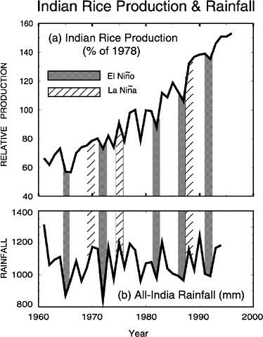
FIGURE 3.1 Relationship of Indian rice production to Indian rainfall. Production in 1978 = 100. SOURCE: Webster et al. (1998); adapted from Gadgil (1995). Courtesy of the American Geophysical Union.
(SOI)—that is, the pressure difference between Tahiti and Darwin, Australia 7—and the AIRI, is plotted in Figure 3.2b. Generally, warm events in the tropics are associated with deficient rainfall, while cold events appear to be related to abundant rainfall.
The relationship between ENSO conditions and the Indian rice yield suggests a number of questions:
-
Although the relationship between ENSO conditions and Indian rice yield is not perfect, it is regular enough to raise the tantalizing suggestion that macroscale variations in the climate system influence variability on the
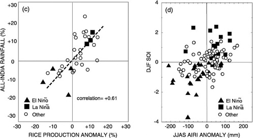
FIGURE 3.2 Scatterplots of (a) AIRI and crop production relationship, depending on their values' percent deviation from the mean, and (b) relationship between AIRI and preceding winter SOI index. (See text for further explanation.) SOURCE: Webster et al. (1998). Courtesy of the American Geophysical Union.
-
smaller scale of India and South Asia. How is this connection manifested in the physical system?
-
Do irregularities in the ENSO/crop yield relationship indicate that intra-seasonal rainfall variability (e.g., the timing of the onset and first break of the monsoon in a particular summer, relative to plowing, planting, and harvesting) also influences total crop yield?
-
Do the irregularities in the relationship between SOI and AIRI suggest inherent limitations in their linkage? What are the factors involved in any such limitations?
-
How accurate must a seasonal forecast of monsoon rainfall be to be of use to the user community? How far in advance would a forecast have to be made?
In the preceding discussion, Indian crop yield is used as an example of the importance of discerning the ways that macroscale climate variability affects the local scale. The questions raised above are common to the monsoon regions of Australia, Africa, and the Americas.
Snow-Monsoon Interactions
In an effort to predict monsoons over a century ago, it was speculated that the varying extent and thickness of Himalayan snow exert some influence on the climatic conditions and weather over the plains of northwest India.8 Himalayan snow was therefore assessed via snowfall reports from various locations in the western Himalayan range as one of the predictors of Indian monsoon rainfall.9 Greater winter snowfall was found to be related to below-normal monsoon rainfall for the period 1880 to 1920. However, for the subsequent 30-year period, snowfall was highly variable and its relationship with the monsoon was reversed. Its use as a predictor was dropped.
Since the early 1970s, the Advanced Very High Resolution Radiometer (AVHRR) aboard National Oceanographic and Atmospheric Administration (NOAA) satellites has provided a snow cover dataset that is sufficiently accurate for continental-scale studies. Some pioneering work10 examined the snow-monsoon relationship using these satellite data. Several observational studies, some examining the role of Eurasian snow extent, others focusing on the Himalayan snow, suggested an inverse snow-monsoon relationship—that is, the less the snowfall, the greater the monsoon.
In the northern hemisphere snow cover ranges from 7 to over 40 percent of the total land area, making it the most rapidly changing natural surface. Snow cover and snow depth in a particular season can be related to atmospheric circulation of the next season through a series of feedback mechanisms.
The two main physical processes through which snow anomalies may affect climate on a seasonal timescale are the albedo effect and the hydrological ef-
fect. Excessive snow in the early part of winter tends to reduce solar radiation in winter (up to four times compared to bare ground) by increasing the surface albedo, thus resulting in the persistence of colder temperatures (and possibly additional snow anomalies). Thus, holding other processes constant, excess snowfall gives rise to a positive feedback.
In particular, positive snow anomalies over the Eurasian continent in winter and spring lead to colder ground temperatures in the following summer and hence anomalously weak meridional temperature gradients, because a substantial fraction of the solar energy available in spring and early summer would go to melting the snow and evaporating water from the wet soil. This lower land-ocean temperature contrast would presumably lead to below-normal monsoon. The entire scenario would be reversed when winter and spring Eurasian snows are below normal precipitation.
General circulation modeling sensitivity experiments substantiate observational evidence of an inverse snow-monsoon relationship.12 In analyzing the relative role of SST variations and land surface processes on the interannual variability of the Asian monsoon system, it is recognized that the former plays a dominant role.
The quasibiennial aspect of monsoons has been investigated, and it has been noted that monsoons play an active role in determining the anomalous state of the warm-water pool in the western Pacific in the following autumn and winter seasons.13 Studies have also suggested an intriguing three-way interaction between Eurasian snow cover, monsoon, and ENSO.14
Forecasting Seasonal to Interannual Variations in Northeast Brazil
The northeastern part of Brazil (in particular, the state of Cear á) is semiarid, has a rainy season from February to April, and is subject to wide rainfall fluctuations from year to year. Throughout Brazilian history, severely dry periods have been marked by severe social dislocations and mass migrations, which have affected the 30 million people of Ceará and the entire social and economic fabric of Brazilian culture.
Statistical correlations of rainfall with climatic indices15 have indicated that Ceará's rainfall is correlated with SST in both the Atlantic and the eastern Pacific. Realizing the vulnerability of its economy to such interannual climate fluctuations, the state of Ceará, in conjunction with the federal government, established an institute called FUNCEME (Funda ção Cearense de Meteorologia e Recursos Hídricos—Ceará's Foundation for Meteorology and Hydrological Resources) to advise the state on the proper actions to take in anticipation of adverse climatic conditions. FUNCEME has published a monthly information bulletin (Monitor Climático) since 1987 that gives monthly global climatic data, ENSO predictions, and local precipitation and hydrological data.
FUNCEME maintains programs addressing both long- and short-term is-
sues. For the long term it advises on actions to be taken on water resources and distribution, well recovery, crop choices and distribution, soil conditions, and environmental degradation. For the short term it issues forecasts for the rainy season and explicit instructions to the various regions of Ceará about the timing of planting and the crops to emphasize, depending on the forecast of abundant or deficient rainfall.
As a result of these activities, the agricultural output of Ceará has gradually grown more stable, no longer subject to the drastic ups and downs of interannual climatic variability.16 For example, the normal grain output for normal rainfall years in Ceará is 540,000 metric tons. In 1987, before concerted action policies were in place, the response to a poor rainfall year (30 percent below normal) was that grain production for that year was 260,000 metric tons, which led to severe hardship in Ceará and the need for relief by the central governmental. In 1992, however, while the rainfall was equally poor (27 percent below normal), a set of actions in response to a relatively accurate forecast allowed the grain production to be 430,000 tons (see Figure 3.3). Even with a second consecutive very poor rainfall year (again relatively accurately forecast), grain production was 190,000 tons.
Land Surface Factors and Climate Prediction at Less Than Interannual Timescales: The 1993 Mississippi Floods
Terrestrial hydrological-atmospheric coupling processes are reasonably well understood at local scales, and there is increasing understanding on a regional basis. Observational studies and model experiments both suggest that terrestrial hydrological-atmospheric coupling cannot be fully rationalized in terms of local context because the integrated effect of land surface modifies the air prior to its arrival at a specific location.17
At the regional scale, some studies suggest that the type of climatic moisture regime prevalent at the beginning of the warm season may be significantly correlated with the subsequent evolution of both temperature and humidity.18 Early warm season conditions, most likely related to global circulation, can provide the land surface with either more or less moisture relative to the long-term mean. This anomaly may influence subsequent moisture conditions, either locally or regionally, as larger-scale atmospheric circulation becomes less important and local convection (and perhaps moisture recycling) becomes more important in the summer season. Preliminary coupled terrestrial hydrological-atmospheric modeling studies19 tend to support this hypothesis.
Modeling experiments carried out in the context of the Global Energy Water-Cycle Experiment Continental-Scale International Project (GCIP) —specifically using the Atmospheric Model Inter-Comparison Project 's 10-year runs—show that it is possible to provide improved simulation of the mean annual cycle when soil moisture is specified. In practice the soil moisture values used in these runs are estimated from observed temperature and precipitation, rather than from true
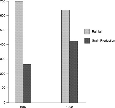
FIGURE 3.3 Grain production (1,000 tons) verses precipitation (millimeters) in Ceará, Northeast Brazil, for 1987 and 1992, both El Niño years. SOURCE: Based on Moura (1994). Data provided by FUNCEME and IBGE/GCEA. Courtesy of the World Meteorological Organization.
soil moisture measurements. Nonetheless, these AMIP simulations suggest that improved specification of soil moisture, and, it might therefore be presumed, improved prediction of the seasonal evolution of soil moisture in coupled terrestrial hydrological-atmospheric models, have the potential to improve seasonal precipitation forecasts.
Dynamical processes controlled by regional water and energy balance can influence vapor flow and in this way may contribute to the occurrence of extreme events. The control of land surface processes primarily arises through their effect on the Bowen ratio, which influences the diurnal evolution of the boundary layer. Land surface processes also have substantial influence on elevated mixed layers and on associated “lids” on atmospheric instability that focus the release of convective instability and hence determine the distribution of regional precipitation in time and space.20
A particularly important issue regarding North America is that the surface energy balance is known to affect the low-level jet over the Great Plains. Such coupling has been demonstrated by numerical modeling and from observations.21 This low-level jet is, in turn, a major factor in the regional moisture transport and moisture flux divergence in the Mississippi River region. 22
The case of the 1993 floods in the Midwest is particularly revealing. Simulations carried out at the European Centre for Medium-Range Weather Forecasting (ECMWF) used two land surface schemes—one with known defects and another with model improvements correcting those defects such that regional-scale soil moisture fields were better represented in the model.23 Predictions made with the version that more poorly represented surface interactions, and thus calculated overly dry soil moisture, provided an unrealistic simulation of the 1993 Mississippi River floods. However, simulations made with the improved representation of surface processes gave a much improved simulation of the persistent rain that caused catastrophic floods and extensive damage in the central Mississippi during July 1993. One study24 concluded, converse to other conclusions,25 that upstream moistening would lead to a weakening of the low-level jet and so act to reduce Mississippi flooding, A follow-up study 26 found that changes in the low-level jet were sensitive to a limited-area model's lateral boundary conditions and that such changes would largely vanish with a large-enough domain.
A RESEARCH AGENDA FOR THE NEXT DECADE
Research Imperatives and Key Scientific Questions
There are five Research Imperatives in studying climate on seasonal to inter-annual timescales:
-
ENSO. Maintain and improve the capability to make ENSO predictions.
-
Global monsoon. Define global seasonal to interannual variability, especially the global monsoon systems, and understand the extent to which it is predictable.
-
Land surface exchanges. Understand the roles of land surface energy and water exchanges and their correct representation in models for seasonal to interannual prediction.
-
Downscaling. Improve the ability to interpret the effects of large-scale climate variability on a local scale (downscale).
-
Terrestrial hydrology. Understand the seasonal to interannual factors that influence land surface manifestations of the hydrological cycle, such as floods, droughts, and other extreme weather.
ENSO Imperative
Dynamical climate predictions began with a 1986 forecast27 and ever since have increased in skill and proven valuable in applications around the Pacific basin and in other regions where ENSO exerts strong control. The field is relatively young, standing roughly at the same place numerical weather prediction did after an initial crude forecast in 1948.28 Coupled models are being developed, data assimilation techniques are being implemented and tested, and various schemes are being used to teleconnect the forecasts of SST to midlatitudes. Forecast systems for the United States are being developed by the National Center for Environmental Prediction, and the concept of end-to-end forecasting is being demonstrated by the newly formed International Research Institute for Climate Prediction. The need now is to proceed.
The following questions are essential to address for progress in ENSO forecasting:
What is the inherent limit of ENSO predictability? How can this limit be determined? What limits the skill of ENSO predictions now? Relatively skillful forecasts of SST in the tropical Pacific are now being made at lead times of one year, with indications of predictive skill for up to two years in advance.29 It is of great interest to know if there is an ultimate limit to predictability in the same way that deterministic prediction of weather is inherently limited to the order of two weeks or so. The limitation is given by how fast errors grow, and this limit can be investigated by examining error growth in models under various circumstances. 30 Performing regular and systematic forecasts is another way of gaining experience with predictability limits, since the inherent limit cannot be less than the skill actually attained. Current forecasts are presumably not near this inherent limit, so it is important to know what constrains current prediction schemes—such as model errors, inadequate data, inaccurate data, or incomplete physical parameterizations.
What mix of observations is needed to initialize forecasts to optimize the skill of ENSO predictions? How can this mix be determined? A prediction must be initialized with the proper state of the coupled atmosphere-ocean system. Currently available data include the TAO array, historical winds from the Comprehensive Ocean-Atmosphere Dataset, sea-level height from altimetry and island stations, subsurface data from expendable bathythermographs, and others. The system has not been “designed” in any sense, so it is possible that a rearrangement of, say, the TAO array could increase skill, as might adding additional moorings or spending more money on some part of the observational system at the expense of others. These questions can be answered in models by performing Observing System Simulation Experiments, in which known model results are subsampled at the observational system points with comparable accuracies. The best observational system maximizes skill.
Which are the proper measures of the skill of ENSO prediction? Current measures of skill are in terms of single indices, in particular NINO3, which is the averaged SST from 5°S to 5°N and from 90°W to 160°E. The correlation of this predicted index with observed and root mean square difference between predicted and observed values of this index, as compared to persistence, is the basis of current skill scores. This definition of skill is oversimplified, but a more acceptable skill score has not yet been developed.
How does decadal variability in the Pacific affect the prediction of ENSO? Long series of hindcasts have shown that skill is not stationary —it varies from decade to decade.31 The persistence skill itself varies decadally. Recent discoveries of decadal modes in the Pacific32 raise the question of whether the decadal variation of skill can be related to physical modes of decadal variability.
Through what mechanisms do seasonal to interannual tropical Pacific variations influence the midlatitudes? It has been known from inferences about the remote effects of ENSO and from modeling studies that SST in the tropical Pacific affects midlatitude regions.33 To develop skill at midlatitudes, it is important to accurately model these remote effects.
What is the relationship between the annual cycle and ENSO predictability? Do models have to get the annual cycle right to predict ENSO correctly? Is there a predictability barrier? The annual cycle is the most reliable and important climatic signal, yet it is not well understood in the tropics. In particular, coupled general circulation models (GCMs) have had enormous trouble getting the annual cycle correct, and this has slowed progress on prediction. On the other hand, the relationship between the annual cycle and ENSO and its prediction are still areas of active research. Early results seemed to indicate that prediction skill dropped off radically during the spring months, but more recent predictions seem to have gotten through the first spring with little loss of skill.
What is the effect of regions outside the tropical Pacific on the prediction of ENSO variations? The simpler models (e.g., the Cane-Zebiak model) include only the Pacific basin yet still manage to attain high skill scores. Some evidence suggests that there are correlations between the Asian monsoon and ENSO and between Atlantic climate and ENSO. Whether these correlations mean that the connections to other basins must be taken into account in predicting ENSO, or whether they are just the remote effects of ENSO, is still not known.
Global Monsoon Imperative
The first question that must be faced in addressing this Research Imperative is the following: What are the structure and dynamics of the annual cycle of the coupled ocean-atmosphere land system, and what are the reasons for its large spatial variability over the globe? The seasonal to interannual variabilities of climate are relatively small fluctuations of the predominant and largest amplitude of all climate variations: the annual cycle. For example, a modest shift in the
wintertime planetary wave configuration can bring below-average and more frequent snowstorms to the United States. A small displacement of the convection associated with the summer monsoon can bring floods or droughts to the semiarid regions that lie along the margins of the monsoon rain belts. Thus, to predict the climate anomaly patterns as they evolve from one season to the next requires a thorough understanding of the annual cycle and an ability to model it. However, the annual cycle is strikingly different in different parts of the world. Phase relationships between the annual cycle and solar radiation are highly variable. Furthermore, the amplitude of the annual cycle in different parts of the globe is very different. The differences in phase and amplitude are caused by different responses of the atmosphere, ocean, and land to thermodynamical forcing and the regional dynamical responses of the coupled system to this forcing.
To date, we can describe the gross features of the coupled ocean-atmosphere-land system, yet we are not so well advanced in modeling this variability. For example, simulating the phase of the annual SST in the Pacific Ocean is still elusive. But to forecast small deviations from the annual cycle, it must be keenly modeled.
What is the nature of global interannual climate variability, and what is its relationship to the annual cycle? What processes give rise to such variability? Can our increased understanding of this variability be exploited for prediction? The ENSO cycle is the dominant mode of interannual variability in and over the Pacific Ocean. The TOGA program has established that ENSO variability is the result of coupled ocean atmosphere processes. Additionally, the ENSO cycle is phase locked with the annual cycle, although there is recent evidence that this locking tends to shift on interdecadal timescales. Rather robust theories have been developed to explain the coupled ocean-atmosphere dynamics that produce ENSO, but why ENSO is phase locked at all with the annual cycle is less well known. It has long been established that there is interannual variability in other parts of the globe, especially in the monsoon regions. Some of this variability appears to be connected to ENSO. It is not known, however, whether there are other large-scale forcing functions (e.g., variations in ground moisture, winter snow cover) or whether there is a chaotic component to the monsoon. Clearly, though, advances in predicting interannual variability must begin with a more thorough description and understanding of the climate system.
What are the roles of slowly varying conditions at the Earth's surface (sea ice, SST, snow cover, and soil moisture) in determining the nature of interannual variations in the global atmosphere? It has been hypothesized that in the extratropics there is little predictability beyond a few weeks because the circulations are dominated by short-term hydrodynamical instabilities, which, from a climate perspective, are essentially unpredictable. It is generally believed that in the tropics, there are no hydrodynamical equivalents to baroclinic instabilities. Thus, it has been hypothesized that the interannual variability of the tropics should be determined by the slowly varying boundary conditions, especially the SST varia-
tions associated with ENSO. To a large degree this appears to be a robust result. Yet in the monsoon regions there is some evidence of dynamically unstable modes. Whether such modes reduce the predictability of the monsoon has not yet been determined.
In the continental regions of the higher latitudes (e.g., the United States), anomalies in soil moisture can persist for periods longer than a season. At higher latitudes there are long-lived sea ice and snow cover anomalies as well. Whether these extratropical anomalies can nudge the chaotic dynamics to some preferred state, and thus add predictability to the system, has yet to be determined.
What determines the low-level convergence of moisture in the tropics over water, land, and coasts? More generally, what determines the location and longevity of the heat sources and sinks of the atmosphere? The heating gradients between the heat sources and sinks of the atmosphere determine the basic circulation haracteristics of the coupled climate system. Heat sources are generally related to regions of latent heat release and are usually located over the warm tropical oceans or tropical land areas. Heat sinks are associated with radiative loss to space. The subtropical continental desert regions and the subtropical highpressure regimes over the oceans are heat sinks. The greatest and most persistent heat sink exists over North Africa and the Middle East. The heat sources are formed in a cooperative manner. It is thought that the convergence of moisture is caused by surface heating of the atmosphere either over the tropical ocean warm pools or the heated continents. The release of latent heat in these regions defines the heat source. During the year, the heat sources tend to migrate following the Sun but with different rates of progression depending on their relationship with the ocean or the land. We are fairly certain that major heat sources and sinks are not independent, and it appears that they interact. But how they interact and modify one another is not known. Nor is it known how these interactions produce rainfall anomalies, which are often on scales that are less than the scale of the sources.
What is the role of ENSO in creating variability in the monsoon climates of the world and vice versa? For over 100 years it has been apparent that the Asian-Australian monsoon system undergoes aperiodic and high-amplitude variations. Often (but not always) the monsoon variability appears to move in synchronization with interannual ENSO variability in the Pacific Ocean. At other times there appears to be only a weak relationship or none at all; at still other times monsoon variability appears to lead ENSO. These associations between ENSO and the monsoon are real but exactly how the two systems relate physically is still not fully understood.
Is there variability of the monsoon that is independent of ENSO and is it predictable? The Southern Osilation Index (SOI) explains about 45 percent of the variance of the Indian summer rainfall. Clearly, other factors must be important. One possibility is the snowfall over Eurasia during the previous winter and spring. If there is abundant snowfall, the ground surface processes are affected, so
that warming of the Asian continent is retarded. Possibly this leads to slow formation of the monsoon trough over India. There are SST anomalies in the Indian Ocean although they are usually a factor of two smaller than those found in the Pacific Ocean associated with ENSO. However, the impact of these anomalies has not been fully explored, especially as they relate to regional aspects of the monsoon. Possibly, there may be an unpredictable component in the monsoon structure. In this theory the SST anomalies associated with ENSO control the macroscale monsoon to a large degree, tending to render the monsoon anomalously wet or dry. However, hydrodynamical instabilities in the monsoon system (if they exist) would add an unpredictable element to this large-scale control. At this time the role of such boundary forcing factors or the introduction of such uncertainty into predictions of the monsoon system is not understood.
What is the nature of tropical-extratropical interactions? Specifically, how might tropical SSTs perturb the extratropical atmosphere, thereby generating extratropical SST anomalies? For what regions of the globe can accurate predictions of tropical SSTs be translated into skillful regional climate forecasts for one to two seasons in advance? The general view is that, compared to the tropics, there is little if any predictability inherent in the extratropical system on seasonal to interannual timescales. The predictability that does exist at higher latitudes results from the atmospheric response to tropical SST anomalies that exert their influence through teleconnection patterns. Extratropical SST anomalies appear to be forced by these patterns. In turn, the extratropics can exert a stochastic forcing on the more predictable tropics. How much tropical predictability may be reduced by this influence is unknown.
What is the role of intraseasonal variability on seasonal to interannual variability? How predictable are the amplitude, distribution, and frequency of blocking, and active and break periods of the monsoon? Intraseasonal variability is an important element of tropical and extratropical climates. For example, active and break periods of the monsoon produce variability in rainfall on timescales of 10 to 30 days. Timing within the monsoon climate is critical, as even in a good monsoon year an “ill-timed” break can have devastating consequences. Blocking at higher latitudes modulates weather for long periods of time. Yet the physical processes that produce intraseasonal variability have not been identified. Nor are these processes simulated or predicted with sufficient accuracy in numerical models. The manner in which intraseasonal variability affects seasonal to interannual variability, or vice versa, also is unknown.
Land Surface Exchanges Imperative
Five general Scientific Questions need to be explored to investigate land surface processes involving energy and water:
What is the appropriate level of detail in characterizing land surface for
seasonal to interannual prediction, with regard to (1) the nature of vegetation and soil parameters and their specification, (2) the spatial resolution in observing vegetation and soil, and (3) description of seasonal changes in vegetation cover and its vigor? Vegetation influences several aspects of the hydrological cycle. There is long-standing evidence that vegetation cover affects catchment runoff, and the interception of rainwater by canopies and its rapid reevaporation are recognized as important in this. Foliage is known to exert biological control on transpiration by regulating the stomatal pores through which water vapor leaves a plant. The morphology of plant canopies also influences the absorption of solar energy and the generation of turbulence. These factors together influence the energy balance between radiant energy, sensible heat and latent heat, and heat flow in the soil. The sensitivity of stomata to soil moisture change is small when soil moisture is high but is a strong control on transpiration when soil moisture is low.
The nature of the underlying soil is also important to land surface hydrological-atmospheric coupling. Infiltration of water in the soil surface (which can be modified by root growth and soil tillage) influences how much precipitation enters the soil and how much runs off to river systems. Soil parameters in the vegetation rooting zone determine the amount of water that can be released to the atmosphere during a long dry period and how much water percolates to groundwater.
Modern biosphere-atmosphere models can simulate complex soil-vegetation-atmosphere interactions realistically, and model sensitivity studies confirm that realistic description is indeed necessary when simulating climate over decades and longer. It is not yet clear what level of realism is appropriate for seasonal to interannual climate prediction. Climate models adopt alternative approaches when specifying vegetation and soil parameters. Some models assign values according to the nature of the local land cover ascribed to areas in globally specified land cover maps, while others specify the value of individual parameters globally. The relative merits of these two alternative approaches for seasonal to interannual prediction also are not known.
Over the past decade, substantial progress has been made in understanding how to represent subgrid-scale heterogeneous land cover and thus representation of surface energy partitioning in climate models for long-term prediction. Meanwhile, rapid progress has also been made in obtaining remotely sensed land cover data to apply that understanding. No attempt has yet been made to apply this knowledge at seasonal to interannual timescales.
To operate, biosphere-atmosphere models must be supplied with or generate information on leaf area and its seasonal development. Model experiments reveal that predictions are sensitive to vegetation type and cover. Currently, seasonal to interannual predictions must assume specified seasonal behavior for these variables, but models that simulate seasonal growth and senescence may be preferable.
What representation of runoff is best to calculate evapotranspiration in seasonal to interannual climate prediction models? Models used for seasonal to
interannual prediction must simulate surface water balance realistically to calculate the seasonal evolution of evapotranspiration accurately. To model surface water balance well, they must provide appropriate descriptions of runoff processes. However, in the past, climate models have paid meager attention to representing this aspect of the land surface hydrological cycle, and greater emphasis must be given to modeling runoff in coupled hydrological-atmospheric models, and to validating the modeled runoff against observations.
What is the appropriate form for the land component of a four-dimensional data assimilation system for seasonal to interannual prediction? What are the appropriate measurements and tradeoffs? How can they be obtained and how can models be formulated to accept them? It is more important that seasonal to interannual climate models are accurately initiated, as compared to longer-term prediction models. Correct initiation of state variables in hydrological-atmospheric models is thus important, while initiation of soil moisture status in such models is critical. In this regard there is potential value in using four-dimensional data assimilation procedures to initiate models, when using observations of nearsurface soil moisture from spaceborne L-bandb radiometers. Meanwhile, model-calculated soil moisture fields must be used in initiation, seeking improvements in them by improving the realism of the model and the reliability of the model inputs used in the calculation.
How can we use observations of seasonal to interannual variations in biogeochemical cycles and ecosystem properties to infer the underlying dynamics determining these variations? Over the past decade, noteworthy progress has been made in using networks of in situ concentration measurements to determine the location and seasonality of trace gases in the global atmosphere and in using remotely sensed data as an indirect measure of seasonal variations in ecosystem properties. These integrating measurements have potential value in validating the representation of seasonal features in ecohydrological models.
What is the role of high-latitude feedbacks between snow cover extent, streamflow, and seasonal to interannual variability and to what extent are these processes adequately modeled? The extent of snow and ice varies markedly from year to year, which can have a major impact on the global radiation budget because of the associated change in the surface reflectivity for solar radiation. At high latitudes and high altitudes, surface water stored as snow and ice during the winter season is released as streamflow, to return to oceans in the subsequent spring and summer, thus providing a means for achieving freshwater balance between seasons. The presence of an energy-related storage mechanism in the Earth's water budget provides opportunity for seasonal feedback, which may be poorly modeled in predictive models.
|
b |
The L-band is the nominal frequency range from 2 to 7 Ghz (20 to 76 cm wavelength) within the microwave (radar) portion of the electromagnetic spectrum. |
Downscaling Research Imperative
Downscaling—interpreting the effects of large-scale climate variability at the local scale—lies at the heart of meeting users' requirements. For successful downscaling, two key questions must be resolved.
In what ways can local climate variance be explained in terms of large-scale climate variability? Transformation of large-scale GCM climate predictions to regional and local areas is critical to interdisciplinary scientists and others who wish to know the impacts of climate variability on their areas and activities (e.g., water resources, agriculture, urban development). As already noted, the influence of many factors, such as topography and land cover, determines whether any change predicted at a typical GCM grid size projects down to local land surface scales in a linear way. Three methods have been used to address this issue. The first approach is the empirical and statistical method, called a Weather Generator, which derives a correlation between a specific local climate variable (such as precipitation) and an appropriate measure of large-scale climate variability (such as the height of a 500-mb pressure surface). The availability of reasonably long historical records of the variables is essential to this approach. The second approach is a dynamic method of nested modeling, which increases the spatial resolution for the study region in a GCM. A third approach is to use a nested regional model that is forced at its boundary by GCM results. Each approach estimates changes in the local climate variance that are related to large-scale (GCM-scale) climate variability.
Current methods rely on additional scaling knowledge, either from observation or dynamics, to complete the transformation. Therefore, any enhancement of these methods will require improved descriptions of related physical processes at high resolution and through the use of remote sensing data.
The second question deals with “upscaling” local variables for use in large-scale models: What local climate variables need to be upscaled to ensure adequate coupling of local climate to large-scale climate? Although the role of land surface in the climate system was always thought to be important, until recently most atmospheric modelers believed that it played only a minor role in influencing climate variability. New research reported in connection with the GCIP program has changed this perception. Recent improvements in the new ECMWF model, in simulating the heavy 1993 rainfall over the upper Mississippi River basin, have been attributed to the use of a new land surface scheme;34 this has helped to increase the GCM modeling community's interest in the potential influences of the land surface. The recent emphasis on improving land surface parameterization (LSP) schemes is a move in the right direction. However, there are still many unresolved problems with LSPs. A major problem is related to the horizontal subgrid parameterization of processes that control surface energy and water fluxes. The current generation of LSPs use a point or patch representation of the land surface, with effective parameters, at the mesoscale or GCM grid
scale. All the heterogeneity of the land surface is assumed to be subsumed into these effective parameters. The most immediate consequence of this assumption is the implication that runoff production is linear with scale. This is clearly not the case, given that only parts of the land surface are responsible for runoff production. It is therefore critical that the effects of heterogeneity in inputs, soil characteristics, and antecedent moisture be appropriately represented in LSPs, so that adequate coupling of local climate to large-scale systems can be established. A reasonable description of runoff, to allow direct GCM simulations of climate variability effects on river discharge, will be critical to the hydrological and water resources communities.
The horizontal heterogeneity discussed above also influences and is influenced by the vertical mechanisms of the transport of energy, water mass, and momentum from the Earth's surface to the lower boundary of the atmosphere known as the planetary boundary layer (PBL). The vertical transfer mechanisms between the land and the PBL occur at spatial resolutions much finer than the typical GCM grids.35 Relatively minor improvements in the PBL models and parameterization have been made to date. Additional research focused on PBL transport response to land surface variations will most likely provide the critical insight needed to improve LSPs and hence the coupling of local to large-scale climate.
Terrestrial Hydrology Imperative
Seasonal to interannual forecasts of hydrologically important surface variables (especially precipitation and temperature) could be incorporated into hydrological forecasts (in particular of streamflow), which in turn could have important benefits for water managers. However, important Research Questions remain in making the transition from surface climate to hydrology. These questions reflect mismatches in spatial scale and the sensitivity of predictions of the hydrological system to even modest biases in surface climate forecasts. These research questions include the following:
What are the implications of seasonal to interannual climate forecasts for flood prediction? Opportunities exist in several areas. With respect to flash floods (the severity of which is usually controlled by the intensity of precipitation over relatively small watersheds), there is potential for predicting changes in flood risk (e.g., the magnitude of the n-year flood) depending on the current (or forecast) climate state. This capability is distinguished from the forecasting of particular flood events at seasonal to interannual timescales, which is unlikely to be feasible for the foreseeable future. Likewise, it may be possible to predict the risk of rain-on-snow floods in the maritime mountainous environments of the western United States, although prediction of specific events at seasonal to interannual timescales is unlikely to be feasible. On the other hand, for floods in
large continental river basins, it may be possible to predict the evolution and timing of specific flood events. This is particularly true for situations in which antecedent conditions (such as soil moisture and snow moisture storage) exert a strong influence on future runoff. The skill of climate forecasts should be evaluated with respect to precipitation, including statistical descriptors of its space-time evolution. Similarly, for spring snowmelt floods in the mountainous west, forecasts of winter precipitation and temperature might be used in conjunction with hydrological models to predict the evolution of spring snowmelt. But important questions still remain about the ability of climate models to predict the coincident evolution of precipitation and temperature that controls the buildup of the winter snowpack.
What are the implications of seasonal to interannual climate forecasts for drought prediction and forecasting? Three kinds of drought can be distinguished. Meteorological drought can be specified in terms of accumulated precipitation anomalies. Therefore, the value of seasonal to interannual climate forecasts for predicting meteorological drought is directly related to their skill in forecasting precipitation. Agricultural drought is defined in terms of soil moisture deficit (e.g., from field capacity), which is related to the accumulated difference between precipitation and evapotranspiration. Therefore, agricultural drought is determined by a more complex interaction of evaporative demand (which in turn is a function of net radiation, wind speed, and vapor pressure deficit) with precipitation and initial soil moisture. Hydrological drought is defined in terms of streamflow (perhaps averaged over an appropriate time period). Hydrological drought is governed by variables similar to those of meteorological drought, but they interact in a more complex manner. For instance, streamflow is conceptualized in many models to be derived from two sources: surface runoff production, which is related to instantaneous precipitation intensity and local surface soil moisture, and drainage, which is defined over longer timescales by soil moisture (and/or groundwater) at depth. Under drought conditions, drainage (manifested as baseflow, which is primarily the groundwater contribution to streamflow) dominates. Therefore, hydrological drought is determined by the complex interaction of processes that lead to deep soil moisture, and/or groundwater characteristics, throughout the forecast period.
What are the implications of seasonal to interannual climate forecasts under “normal” climate conditions? Seasonal to interannual forecasts may offer considerable benefits for improved water-use efficiency under “normal” conditions. Especially in the western United States, where streamflow is fully appropriated, water management issues almost always exist, not just during extreme years. For instance, in streams where water rights are fully appropriated (as in much of the western United States), junior water users are not entitled to irrigation water until senior users have been satisfied. Therefore, these users could benefit from more accurate information about streamflow at seasonal to interannual lead times, which may determine whether, and what, crops are planted. Likewise, hydroelectric power operations are critically dependent on information about future
streamflows because the value of the power generated depends on how far in advance contractual commitments can be made for power delivery. Navigation, recreation, and environmental activities (including fisheries protection and enhancement) could also enjoy economic and other gains, if future information about streamflow (and/or reservoir releases) were available. Methods of using seasonal to interannual climate forecasts under these conditions may well have greater long-term economic benefit than forecasts under less frequent flood or drought situations.
LESSONS LEARNED
Four central lessons emerge from experience with TOGA and with ENSO prediction.
-
A close relationship between models and observations is the clearest way to progress. One of the key lessons learned from the TOGA program was the fruitful and reinforcing relationship between models and observations. It showed that a balanced approach to modeling and observations was the surest way to progress and that both observations without models and models without observations were inadequate.
Linear models of the response of the equatorial thermocline to winds were worked out by the early 1980s, allowing quantitative tests of the theory, something really quite new in oceanography. Measurements of the thermal structure of the equatorial ocean were taken, yielding a good indication that the large-scale structure of the thermocline could be understood in terms of the large-scale structure of the winds.36
The development of ENSO prediction also forced a fruitful confrontation between models and observations: observations were absolutely required to initialize the predictions, and the constant need to evaluate the predictions' accuracy required constant comparisons of the model to the verifying observations. Initialization required assimilating data in the model, and this demanded that the model be good enough to accept the data; if not, the data require that the model and/or assimilation procedure be improved. Once the model is good enough to assimilate the data, the initial analysis gives a view of the system that would be impossible from the data alone. The case is much like weather prediction, except that ocean data were essential to initialize the forecasts, and fields of ocean model-assimilated data are the products of the analysis procedure.
-
The ocean and land are woefully undersampled, with resulting major lacunae in understanding, simulation, and prediction. There are many parts of the deep ocean where no instrument has ever recorded an observation. Even at the surface, some parts of the Southern Ocean have never been sampled. The equatorial Pacific is only sparsely traveled by volunteer observing ships. Thus, the long-term surface database (COADS—Comprehensive Ocean-Atmosphere
-
Dataset) did not allow complete study of surface interannual variability over the ENSO region. The research community depended instead on interpolated wind fields from relatively sparse sampling (in time and space) to force the ocean models. Fortunately, the large-scale behavior of the ocean could be described by relatively crude wind fields, so that progress was delayed but not short-circuited altogether. The demands of prediction, however, require a better dataset: it was not until the establishment of the TOGA TAO array that the surface meteorology became better established.
Lacking a long-term dataset in and over the ocean means that the variability of SST, both interannual and on longer scales, remains unknown over large reaches of the ocean. It is just such a lacuna that the U.S. Global Ocean-Atmosphere-Land Surface (GOALS) program is designed to address. The current combination of satellite and in situ measurements, if maintained both continuously and permanently, will lead to a global SST dataset with few gaps. Because the satellites that provide SST are routinely used in weather prediction, the likelihood that this will happen is good. For other surface quantities, such as wind or sea-level height, the prospects are not as good. Such measurements are extremely valuable, but they are not in the operational domain, so there is no requirement (or intention) that they be permanently maintained. In fact, no institution is responsible for long-term measurements outside the domain of weather prediction, no matter how valuable these measurements may be for the climate record.
For measurements beneath the surface of the ocean, the situation is rather bleak. At only two isolated sites in the ocean are long-term (point) measurements taken, from the weather ship Mike (in the Norwegian Sea) and the Bermuda station. The TAO array is the first measurement system deployed in the world's oceans that is designed to permanently measure quantities of vital interest to the prediction community and by extension to the oceanographic community. How to maintain the TAO array when no operational agency has responsibility for it is a problem that has occupied the research community in seasonal to interannual prediction for several years.37 The problem is in fact generic: no operational agency supports any measurements other than those taken for weather prediction.
-
Scientists from different fields work together most productively and smoothly when the problem demands it—and global change demands it. There is much talk about the value of interdisciplinary studies, but it has proven difficult to encourage people in different fields to work together. In global change research, however, people from entirely different fields, such as meteorology and oceanography, have worked together smoothly and without prompting because the problem requires their cooperation. The ongoing work on ENSO shows this to be the case. The relatively few people who work between fields, and who show that multiple fields are sometimes essential to find solutions, are the true innovators of interdisciplinary studies.
The decadal climate problem is the kind of problem that demands expertise
in a wide variety of fields. A climate model must have land, ocean, atmosphere, and cryosphere components. Chemical processes must also be encompassed to determine such features as the concentrations of major constituents and the radiative properties of gases, aerosols, and clouds. Land processes expertise is needed as well to characterize the vegetative cover and the marine biological processes that determine the uptake and sequestration of CO2. Thus, the modeler must be a master of all trades.
Similarly the study of ENSO requires knowledge of the convective properties of the atmosphere and how surface winds are generated and altered. It has required understanding of the response of the ocean to such atmospheric changes in terms of thermocline depth changes and, in general, understanding of the interaction of the atmosphere and the ocean in affecting SST.
The lesson is that, wherever barriers are raised, ways must be found to enable people who wish to collaborate with those in other fields in solving specific problems to work together. This may involve more than physical scientists working together—the application of seasonal to interannual prediction requires physical and social scientists to collaborate. The barriers to such collaboration exist in universities, government, and funding agencies.
-
Systems of interest (e.g., agriculture, fisheries, water management) are physical, political, and social; such systems must be studied in both physical and human dimensions. To use seasonal to interannual climate forecasts to our advantage, the identification of applications and the methods of using and communicating the forecasts must be carefully researched. In doing this it is vital to realize that most systems we intend to benefit can only be understood in terms of their normal workings.
The simplest systems are not nearly as simple as is usually assumed. Agriculture depends not only on seeds, sunlight, and water but also price supports, capital availability, opportunities for alternative work nearby, the technological sophistication of the farmer (including knowledge of new varieties and hybrids of seeds and animals), the existence of cooperatives, the care with which the farmer has tended the land, communications of weather and climate information, availability of educational facilities nearby, accessibility of pest control weapons —and still other factors. Agriculture has clear human dimensions that must be understood.
RESEARCH IMPERATIVES: PRIORITIES FOR OBSERVATIONS, MODELING, AND THEORY
Earlier we identified five Research Imperatives that must guide the next decades of research into the interannual timescaies of the climate system:
-
ENSO. Maintain and improve the capability to make ENSO predictions.
-
Global monsoon. Define and predict global seasonal to interannual variability, especially the global monsoon systems.
-
Land surface exchanges. Understand the roles of land surface energy and water exchanges and their correct representation in models for seasonal to interannual prediction.
-
Downscaling. Improve the ability to interpret the effects of large-scale climate variability on a local scale (downscale).
-
Terrestrial hydrology. Understand the seasonal to interannual factors that influence land surface manifestations of the hydrological cycle, such as floods, droughts, and other extreme weather.
ENSO Research Imperative
The development of short-range (seasonal to interannual) climate prediction during TOGA has opened the doors to a new age of possibilities. It is not hard to imagine short-range climate prediction finding its place in the economic apparatus of modern industrial society, by providing valuable information about the future that can be used to economic advantage. Short-range climate prediction for the United States is in its infancy but through careful nurturing could be brought to maturity.
The key to developing better forecasts is a balanced combination of modeling, observations, and continuing research. It is absolutely essential to maintain the TAO array and other tropical Pacific observing systems until their value can be more carefully assessed, with reference to the objective standard of skill in prediction. Also crucial are continuing efforts to develop “end-to-end” prediction, in which predictions are not only made but used, evaluated, and improved, and the applications of the predictions also pass through such developmental stages. Additionally, demonstration projects are needed to learn how forecasts are used and how to increase their effectiveness. These demonstration projects do not have to be focused on the United States; they could initially be carried out in regions for which predictive skill is higher, particularly in countries around the tropical Pacific. The newly formed International Research Institute for Climate Prediction should be encouraged to develop these demonstration projects. Finally, commitment to the Program for Climate Variability and Predictability (CLIVAR)/GOALS and the Global Energy and Water Cycle Experiment will assure that the research needed to advance seasonal to interannual climate prediction will be done.
Observational Requirements
The ENSO prediction process—predicting aspects of SST and corollary variables—requires data to initialize the coupled models and data to evaluate the skill of the predictions. Because SST is the crucial variable in making predictions,
weekly fields of SST at the one degree by one degree level are absolutely essential. These are currently provided by AVHRR measurements, combined with in situ drifters to pin down the absolute values and gradients of SST. The key variables for initializing the model are the state of the atmosphere and the density state of the upper ocean. The state of the atmosphere does not seem to be as critical for initialization, since the model atmospheric state rapidly adjusts to the initial SST. In any case, the state of the atmosphere is provided by the twice-daily analyses from the operational weather prediction models.
The internal state of the upper ocean can be assessed in two separate ways: directly by temperature-measuring instruments, on a line connecting a surface mooring to a bottom anchor, or indirectly by applying observed heat and momentum fluxes over the ocean component of the coupled model for a long period of time (usually exceeding 20 years). In practice, salinity is very difficult to measure and does not make a major contribution to the initial thermal state, so the direct method measures only temperature. The indirect method depends primarily on measuring the momentum fluxes with the heat fluxes parameterized, so that only the surface winds are used in the calculation.
Currently, ocean models are initialized by combining the two methods above, by assimilating both the long-term history of the wind fields and the currently obtained thermal state of the upper ocean, to arrive at an optimal estimate of the ocean's current thermal state. The subsurface ocean data are provided by a network of 70 moored TAO arrays in the tropical Pacific Ocean (providing approximately 2 degrees of meridional resolution and 15 degrees of longitudinal resolution). These same moorings measure winds, but, since the full TAO array has been in existence for only two years or so, historical winds must be obtained from the COADS dataset, gathered from individual ship reports from volunteer observing ships.
Because the TAO array measures the quantities needed to initialize the ocean component of the predictions, it is vital that this array be continued. The TAO array was designed on the basis of the scales of variability of the winds. It may turn out that either fewer or more moorings are required to optimize prediction skill. Other quantities also prove useful for initialization:
-
Sea surface height, as measured by satellite altimetry and by tide gauge stations scattered around the islands and coasts of the tropical Pacific.
-
Currents measured on the equator, where geostrophy is more problematic.
-
Cloud cover and solar irradiance reaching the surface.
-
Precipitation in those areas in and surrounding the tropical Pacific (and remotely in the areas that ENSO affects) to evaluate the skill of precipitation predictions.
-
Upper-level water vapor to evaluate the effect of seasonal to interannual variability, as opposed to greenhouse feedback of this quantity.
The overall recommendation, therefore, is to maintain global SST measurements and to maintain the TAO array.
Modeling Requirements
The National Research Council panel on the GOALS component of CLIVAR has made the following recommendations for developing improved models:
Improvements are needed in all of the component models of the climate system in order to increase prediction skill in the seasonal to interannual time frame . . . . Atmospheric general circulation models need to be improved to a stage where, when driven with prescribed observed SST, they simulate realistically the observed annual cycle and interannual variability of the surface wind stress and heat flux, as well as the global atmospheric circulation and rainfall. . . . Similarly, oceanic general circulation models need to be improved to a stage where, with prescribed surface stresses and heat fluxes, they simulate realistically the observed annual cycle and interannual variability of SST, upwelling, upper-ocean heat content, convection, and subduction. The improvement of land surface process models (LSPMs) to a stage where they represent adequately the interaction between the land surface and vegetation and the atmosphere is necessary.38
The panel especially acknowledges the need for developing an integrated approach to modeling seasonal to interannual climate change and notes that:
In addition to improving the individual component models of the climate system, the panel recommends an equally strong effort in coupling the component models together so that they better approximate the natural system. . . . Though somewhat simpler than GCMs, models of intermediate complexity should also be constructed. . . .
With regard to applications and human dimensions, the panel recommends that auxiliary models be designed to predict societally important quantities not routinely produced by seasonal to interannual climate forecast models. . . . Auxiliary models include those used to make projections of agricultural yield, water availability, fish productivity, energy demand, economic impact, and so on. . . .
Improved strategies should be developed for nesting high-resolution regional models and global climate models to infer detailed structures of regional climate anomalies forced by global boundary conditions predicted by coupled ocean-land-atmosphere models. Furthermore, the systematic and periodic intercomparison of models should be continued in order that the physical sciences and the user communities have available an ongoing assessment of the status of models. . . .
Global Monsoon Research Imperative
During the TOGA decade, a concerted effort was made to exploit the predictability that had been found in the coupled ocean-atmosphere system of the Pacific Ocean. Monitoring of the ocean and the atmosphere has provided data for diagnostic studies that have helped in understanding the processes that produce the El Niño and La Niña phenomena. Process studies have been conducted to explore physical associations that were difficult to understand but which were critical links in describing the totality of the phenomena. Numerical coupled ocean-atmosphere models have been constructed, with moderate success in forecasting seasonal to interannual variability in the tropical Pacific Ocean. However, for many years it has been apparent that there are predictable elements in other regions of the tropics as well. The existence of these elements may be seen in the relative success of empirical techniques in foreshadowing interannual variations in the summer rains of the Asian-Australian monsoon.
A major research imperative is to extend the successes of TOGA to the global domain. Of high priority is extension of the monitoring, modeling, and pilot studies of the Pacific Ocean to encompass the other major heat sources and sinks in other tropical oceans and tropical land masses. The principal aim would be to identify predictable elements in these regions and also to determine links with predictable ENSO elements, if they exist. Predictability of the extratropical circulations also should be sought. This goal will be accomplished by following predictable elements that have their roots in the tropics (e.g., ENSO) while at the same time seeking predictable elements that are inherent to the higher-latitude climate system. If inherent extratropical predictability does exist, it would probably come from climate memory associated with low-frequency ocean dynamics or hydrological processes over the land regions.
Observational Requirements
The U.S. GOALS program has devoted much effort to defining the observational requirements for global seasonal to interannual predictions. These requirements are summarized in Table 3.1, which is taken from A Scientific Strategy for U.S. Participation in CLIVAR/GOALS.39 Note that variables are listed in priority order. Not surprisingly, there is considerable overlap between these variables and those identified as important in pursuing the other Research Imperatives identified in this report.
Land Surface Exchanges Research Imperative
Exchanges of water and energy at the land surface are major controls on the hydrological cycle. How evaporative and sensible fluxes interact with the atmo-
TABLE 3.1 State and External (or Forcing) Variables that Must Be Measured for the GOALS Program
|
Realm |
State Variables |
External Variables |
|
Ocean |
Upper-ocean temperature. Upper-ocean currents. Sea level. Upper-ocean salinity. Optical absorption. Sea ice extent, concentration, and thickness. |
Wind stress. Net surface solar radiation. Downwelling long-wave radiation. Surface air temperature. Surface humidity. Precipitation. |
|
Atmosphere |
Wind structure. Thermal structure. Surface air temperature. Sea-level pressure. Water vapor structure. Columnar water vapor and liquid water content. Cloud cover and height. |
Sea surface temperature. Net radiation at top of the atmosphere. Land surface variables (see below). |
|
Land |
Soil moisture. Snow cover and depth. Vegetation type, biomass, and vigor Water runoff. Ground temperature. |
Precipitation. Net surface long-wave and short-wave radiation. Surface wind. Surface air temperature. Surface humidity. Evaporation. Evapotranspiration. |
|
SOURCE: NRC (1998). |
||
spheric boundary layer locally, compared to interactions in remote locations, largely determines the occurrence of low clouds, low-level convergence of wind patterns, and deep convection. These fluxes in turn depend heavily on precipitation and solar radiation from the atmosphere. Both the portioning of solar radiation and precipitation at the surface and the amount and ratio of evaporative and sensible fluxes depend on seasonally varying land cover properties related to vegetation. The land surface is highly heterogeneous with regard to these properties, so representing land surface only in terms of properties at the scale of atmospheric models is problematic and of questionable accuracy.
The processes responsible for evapotranspiration are now relatively well understood as a point measure. However, they depend in part on details of soil moisture distribution. These details are largely unmeasured and poorly understood at the scales of climate models. Two particular factors determining soil
moisture levels are especially poorly understood with regard to representation in climate models: how to represent runoff removal from land surface, and what is and what determines maximum water-holding capacity of the land surface. Much of the continental surface outside the tropics has seasonal snow cover and, in some places, frozen soils, which modify the surface hydrological cycle and solar energy absorption. Snow acts as a water reservoir for months or more but can at times release copious amounts of water rapidly.
Greater understanding of land surface exchanges and their representation in seasonal to interannual prediction models will require a combination of process studies, model evaluation exercises, and model experiments. Much of the required activity can be undertaken effectively through the set of continental-scale experiments being fostered by the World Climate Research Programme. Among these experiments, the Global Energy Water-Cycle Experiment Continental-Scale International Project (GCIP) in the United States and the Large-Scale Biosphere Atmosphere Experiment in South America are of particular relevance to the seasonal to interannual component of the USGCRP. However, the knowledge and model improvement provided by these last two continental-scaie experiments must be effectively merged with the results of ocean-atmosphere studies by the GOALS program, to create a coherent U.S. seasonal to interannual prediction program that focuses on the Americas.
Downscaling Imperative
GCMs are currently the primary tools for studies of climate variability and change. Because of computational considerations relating to nonlinear dynamic equations and the current capabilities of supercomputers, GCM global grids have horizontal resolutions on the order of 100 to 250 km. Unfortunately, information generated at that scale (uniformly applied over the grid) is inadequate to describe many small-scale features of importance to the hydrological and energy cycles. A good example concerning atmospheric aspects of the hydrological cycle is the role of clouds. Moist warm air is transported upward in narrow, cloud-scale regions (kilometers), inducing compensating subsidence of cooler air at large scales (hundreds of kilometers). An example related to land surface hydrology is the way that surface and subsurface runoff production is greatly influenced by the spatial and temporal heterogeneity of precipitation inputs, the heterogeneity of soil hydraulic characteristics and flow pathways, and the heterogeneity of antecedent conditions induced by downslope flows and controlled by topography.
While various LSPs have been developed (and are continuing to be developed) to model small- to large-scale interactions, further work is required on the methodologies to desegregate regional model outputs at the scales of hydrological processes. Both LSPs and hydrological models have many parameters that are tuned to the scale of the model. For example, a GCM LSP would use different parameter values than an LSP developed to work at catchment scale with local
historical station data. Current GCMs simulate precipitation with reduced intensity and increased frequency.40 Developing LSPs and hydrological models that will work with a variety of global and regional observational data would be useful for many studies. A stochastic precipitation disaggregation scheme has been developed that redistributes the GCM-calculated grid average precipitation into a subgrid scale to improve the modeled interaction of the atmosphere and land surface.41 The authors demonstrate that this approach provides a more realistic partitioning of precipitation into snow and rain (judged on the basis of ground-based observations) and a spatial distribution that better conforms to the actual observed heterogeneity of rainfall patterns for the areas (of GCM grid size) that were tested. The latter point is particularly important, considering that, for instance, the total annual runoff volume generated in the Colorado River basin is due to precipitation falling over about 10 percent of the total surface area. The importance of the GCM-generated grid average precipitation relating to the region of actual interest is clear, with regard to water resource management issues at local and regional scales.
In addition to the above-mentioned downscaling concerns, complex modeling issues abound in runoff production. For example, the mechanism through which water is partitioned into runoff and infiltration when snow and ice melt is a critical unresolved issue. Most LSPs follow the lead of the prior generation of bucket models in assuming that runoff either instantly vanishes or in a few cases goes directly to the ocean. Flow-routing schemes are required to overcome this deficiency. The GCIP program is attempting to address some of these downscaling issues. Additionally, there is great need to understand the scale dependence of the inputs and outputs as well as how to adjust the scales to give the best possible predictions, so that our capability to interpret the effects of large-scale climate variability on regional and local scales can be improved.
Terrestrial Hydrology Research Imperative
Variations in climate at seasonal to interannual timescales have important implications for terrestrial hydrology. Although precipitation is the most important determinant of key terrestrial hydrological variables (streamflow, soil moisture, snowpack water content, and evapotranspiration), the land surface acts as a low-pass nonlinear filter, so that antecedent precipitation as well as current precipitation play important roles in smoothing the effects of climate variability at these timescales. The implications of land surface processing of precipitation at these timescales are not well understood. For instance, recent work in the Appalachicola-Chattahoochee-Flint (ACF) river system of the southeastern United States suggests that, even though a fairly strong ENSO signal can be detected in precipitation, the signal appears to be filtered out in the streamflow
record, where it is much weaker. On the other hand, in the Columbia River basin, a strong ENSO signal is present in the streamflow record. Although it may be surmised that the links between winter precipitation (which is largely stored as snowpack) and spring-summer streamflow are likely to be more direct in the Columbia than in the ACF, the effects of land surface processing in seasonal to interannual signals in precipitation are still not fully understood. These effects are further complicated by temperature, which affects both rain-snow transition and evapotranspiration. For example, evapotranspiration mitigates the effects on streamflow of warm wet periods (especially in summer) and exacerbates the effects of cold wet conditions. Especially in the western United States, cold wet winters result in much larger snowpacks, and hence greater spring and summer runoff, than do warm wet winters.
For hydrological purposes, seasonal to interannual climate forecasts could have at least two important functions. The first is to forecast the evolution of hydrologically important surface variables (especially precipitation and temperature) using methods such as ensemble forecasting to represent the range of future conditions over the forecast period. There are mechanisms to extend current methods, such as extended streamflow prediction, to use ensemble forecasts of the time series of surface variables. Important research issues in developing this approach have to do with resolution of biases in the climate forecasts (especially for precipitation). Seasonal to interannual forecasts might also be used in a probabilistic (or risk) context. For instance, seasonal to interannual climatic variability might be reflected in changes in the 100-year flood in ENSO versus non-ENSO years. How best to achieve such forecasts remains to be determined, but the general strategy would be based on classification of the current condition and/or forecasts of the evolution of future conditions at the regional scale, combined with retrospective frequency analysis.
Observational Requirements: Land Surface Exchanges, Downscaling, and Terrestrial Hydrology Research Imperatives
The primarily hydrological observational datasets needed in support of the above imperatives can be described as follows.
Streamflow
The U.S. Geological Survey should take steps to ensure the long-term viability of the stream gages in the Hydro-Climatic Data Network, particularly those having at least 50 years of continuous record. Currently, most of these stations are funded cooperatively for a variety of operational purposes and are difficult to sustain for long-term research purposes.
Precipitation
Station Data
The United States must maintain existing long-term stations within the National Climatic Data Center (NCDC) cooperative network, particularly the subset of those stations that make up the Historical Climate Network.
Radar Precipitation Data
The National Center for Environmental Prediction has recently started to archive a merged WSR88-D (Doppler radar)/gauge product (4-km resolution) that covers most of the United States. The suitability of these data for climatological purposes needs to be evaluated, and steps must be taken to ensure the security of the long-term archive of these data and that they are freely available to the scientific community.
Surface Radiation
Only a very small number of stations now operate in the continental United States that collect a full suite of surface radiation observations (the SURFRAD network). The adequacy of this network for studies of seasonal to interannual variability should be evaluated.
Snow
Point Observations
Snow water equivalent point observations are collected primarily at Natural Resources Conservation Service Snow Telemetry sites in mountainous areas of the western United States. The suitability of these sites for long-term climate studies needs to be evaluated (the longest records from these stations date only to the mid-1980s). Snow depth measurements are collected at some NCDC cooperative stations. The feasibility of using some subset of these stations to measure snow water equivalent should be evaluated. The object is to achieve a much more uniform spatial distribution of station-based observations.
Areal Extent
NOAA's National Operational Hydrologic Remote Sensing Center and its National Environmental Satellite, Data, and Information Service (among other entities) produce satellite-based snow areal extent measurements of the conti-
nental United States and the world. These products are currently used for operational purposes but could prove extremely valuable for assessing such interactions as those between the continental extent of seasonal snow cover and largearea circulation patterns. Steps should be taken to ensure that these data are climatologically useful.
Alogrithums
Satellite remote sensing algorithms to estimate snow water equivalent in a manner suitable for global studies (e.g., spatial resolutions of tens of kilometers) have been improved and may be suitable for seasonal to interannual timescale studies, notwithstanding problems remaining for forested areas. These products need to be assessed and archived at (or through) the National Snow and Ice Data Center.
Wind and Humidity
Although these wind and humidity data are collected at NCDC Surface Airways Stations, many of the records are affected by station and instrument changes, and their use for climatological purposes is problematic. Nonetheless, they are critical for computing potential evapotranspiration and provide reference values for approaches that can lead to spatial estimates (e.g., modeling combined with atmospheric profile data or analysis fields). Thus, more attention should be given to the climatological value of these observations.
Surface Air and Skin Temperature
Observations of surface air temperature are critically important to predict evapotranspiration and snow accumulation and melt. Surface air temperature measurements are routinely collected at NCDC cooperative observer stations as well as at National Weather Service manned observing stations. Because air temperature tends to have much higher spatial correlations locally than, for instance, precipitation, maintenance of an adequate station precipitation network should assure adequacy of surface air temperature measurements, provided that these variables are coincidentally collected. Direct observations of surface (skin) temperature are much more problematic. Surface observations have generally only been collected in research projects and are difficult to interpret. Nonetheless, skin temperature is a state variable predicted by most land surface schemes (some schemes predict an effective vegetation temperature as well). Thus, these measurements might be updated as well. Satellite sensors and algorithms can produce global estimates of skin temperature at time frequencies as high as daily; a ground network could play a critical role in
validating and calibrating the long-term spatial records that are now being acquired.
Surface Energy Fluxes
Direct observations of surface energy fluxes (latent heat, sensible heat, and ground heat flux) have hitherto mainly been collected in conjunction with short-term research programs (e.g., the First ISLSCP Field Experiment and the Hydrological Atmospheric Pilot Experiments). However, recent advances in flux measuring instrumentation (see Chapter 2) indicate that their routine, long-term operation is now becoming feasible. A commitment has been made, for example, to continue long-term operation of some of the BOREAS tower flux sites. The instruments required for routine measurement of surface energy fluxes are a subset of those required to make the more difficult measurements of carbon dioxide for ecosystem research. However, in the case of seasonal to interannual studies, there is an additional need for near-real-time data provision. In the course of the next decade, a network of surface energy and carbon dioxide flux measurement sites should be established to characterize seasonal to interannual changes in the surface-atmosphere exchanges for major vegetation types in the United States and perhaps globally.
Soil Moisture
Soil moisture plays a key role in partitioning net radiation into latent, sensible, and ground heat fluxes, particularly in summer. Some studies have indicated the potential importance of feedbacks between soil moisture and climate, especially in the interior of the northern hemisphere continents in summer. Therefore, observation of soil moisture, through ground- or satellite-based observing systems, or both, is of great importance. A few networks in the continental United States collect ground-based point observations of soil moisture, including networks of the Illinois Water Survey and the Oklahoma Mesonet. While there are questions about how point observations of soil moisture can be interpreted in the context of small-scale spatial variability and about the lack of standard instruments, the feasibility of ground-based networks needs to be evaluated. With regard to remote sensing, both active and passive microwave sensors have shown potential in estimating near-surface soil moisture. Furthermore, in combination with modeling, these surface observations might be extended to greater depths. Many issues remain, and problems of soil moisture estimation from satellite sensors are themselves the subject of ongoing research. Nonetheless, passive microwave sensors have demonstrated the capability to map spatial and temporal soil moisture variability at the watershed scale. With a carefully designed sensor system and carefully formulated algorithms, such measurements can be made
from space at the global scale.42 Viable proposals for candidate satellite missions have been developed and should be given careful attention and support.
Vegetation
Knowledge of seasonal and interannual variability in vegetation properties is critical to understanding links between the land surface and climate at seasonal to interannual timescales. Satellite-based estimates of vegetation properties, such as leaf area index and greenness, are now fairly widely used in numerical weather prediction models. Earth Observing System-era developments (e.g., the moderate-resolution imaging spectrometer) will almost certainly improve the quality of these products. A long-term global archive of seasonal variations in vegetation properties must be preserved, along with sufficient metadata to resolve questions about any effects of changes in instruments.
NOTES
1. NRC (1996).
2. ENSO phases, in particular, Rasmusson and Carpenter (1983); northern hemisphere climate, Horel and Wallace (1981).
3. Cane et al. (1986).
4. NRC (1996). The report describes the TAO array and the other remote and in situ measurement systems providing continuously available data in the tropical Pacific, referred to elsewhere in this report as the ENSO Observing System.
5. Adapted from Mooley and Parthasarathy (1984).
6. Parthasarathy et al. (1988).
7. E.g., Trenberth (1997).
8. Blanford (1984).
9. Walker and Bliss (1932).
10. Hahn and Shukla (1976).
11. Shukla (1987).
12. E.g., Barnett et al. (1989), Vernekar et al. (1995).
13. Meehl (1987), Yasunari (1990), Yasunari and Seki (1992).
14. E.g., Khandekar (1991), Meehl (1994), Yang (1996).
15. Hastenrath (1990a, b).
16. Moura (1994).
17. Charney (1975), Charney et al. (1977).
18. E.g., Rind (1982), Mintz (1984), Delworth and Manabe (1989).
19. Koster and Suarez (1995).
20. Benjamin and Carlson (1986), Clark and Arritt (1995).
21. Modeling, McCorcle (1988), Paegle et al. (1996), Beljaars et al. (1996), Betts et al. (1996); observations, Mitchell et al. (1995).
22. Rasmusson (1967).
23. Betts et al. (1993).
24. Paegle et al. (1996).
25. Beljaars et al. (1996).
26. Seth and Giorgi (1998).
27. Cane et al. (1986).
28. Charney et al. (1950).
29. D. Chen et al. (1995, 1997).
30. E.g., Y.Q. Chen et al. (1995).
31. D. Chen et al. (1995, 1997).
32. Zhang et al. (1996).
33. A review is given by Lau (1997).
34. Betts et al. (1993).
35. As discussed by Avissar and Pielke (1989).
36. Busalacchi et al. (1981, 1983).
37. See NRC (1994) for a thorough discussion.
38. NRC (1998).
39. Ibid.
40. Gao et al. (1996).
41. Gao and Sorooshian (1994).
42. Journal of Hydrology (1996).
REFERENCES AND BIBLIOGRAPHY
Avissar, R., and R.A. Pielke. 1989. A parameterization of heterogeneous land surface for atmospheric numerical models and its impact on regional meteorology. Monthly Weather Review 117:2113-2136.
Barnett, T.P., L. Dumenil, U. Schlese, E. Roeckner, and M. Latif. 1989. The effect of Eurasian snow cover on regional and global climate variations. Journal of Atmospheric Sciences 46:661-685.
Battisti, D.S., and E. Sarachik. 1995. Understanding and predicting ENSO. Reviews of Geophysics 33:1367-1376.
Beljaars, A.C.M., P. Viterbo, M.J. Miller, and A.K. Betts. 1996. Anomalous rainfall over the US during July 1993: Sensitivity to land surface parameterization. Monthly Weather Review 124:364-383.
Benjamin, S.G., and T.N. Carlson. 1986. Some effects of surface heating and topography in the regional severe storm environment. Part I: Three-dimensional simulations. Monthly Weather Review 114:307-329.
Betts, A.K., J.H. Ball, and A.C.M. Beljaars. 1993. Comparison between the land surface response of the European Centre model and the FIFE-1987 data. Quarterly Journal of the Royal Meteorological Society 119:975-1002.
Betts, A.K., J.H. Ball, A.C.M. Beljaars, M.J. Miller, and P. Viterbo. 1996. The land-surface-atmosphere interaction: A review based on observational and global modeling perspectives. Journal of Geophysical Reviews 101(D3):7209-7225.
Blanford, H.F. 1984. On the connection of the Himalayan snowfall with dry winds and seasons of droughts in India. Proceedings of the Royal Society of London 37:3-22.
Busalacchi, A.J., and J.J. O'Brien. 1981. Interannual variability of the equatorial Pacific in the 1960s. Journal of Geophysical Research 86(10):901-10,907.
Busalacchi, A.J., K. Takeuchi, and J.J. O'Brien. 1983. Interannual variability of the equatorial Pacific revisited. Journal of Geophysical Research 88:7551-7562.
Cane, M.A., S.E. Zebiak, and S.C. Dolan. 1986. Experimental forecasts of El Niño. Nature 321:827-832.
Charney, J.G. 1975. Dynamics of desert and drought in the Sahel. Quarterly Journal of the Royal Meteorological Society 101:193-202.
Charney, J.G., R. Fjörtoft, and J. von Neumann. 1950. Numerical integration of the barotropic voracity equation. Tellus 2:237-254.
Charney, J.G., W.J. Quirk, S.H. Chow, and J. Kornfield. 1977. A comparative study of the effects of albedo change on drought in semi-arid regions. Journal of Atmospheric Sciences 34:1366-1385.
Chen, D., S.E. Zebiak, A.J. Busalacchi, and M.A. Cane. 1995. An improved procedure for El Niño forecasting. Science 269:1699-1702.
Chen, D., S.E. Zebiak, M.A. Cane, and A.J. Busalacchi. 1997. Initialization and predictability of a coupled ENSO forecast model Monthly Weather Review 125:773-788.
Chen, Y.Q., D.S. Battisti, T.N. Palmer, J. Barsugli, and E.S. Sarachik. 1995. A study of the predictability of tropical Pacific SST in a coupled atmosphere/ocean model using singular vector analysis: The role of the annual cycle and the ENSO cycle. Monthly Weather Review 125:831-845.
Clark, C.A., and R.W. Arritt. 1995. Numerical simulations of the effect of soil moisture and vegetation cover on the development of deep convection. Journal of Applied Meteorology 34:2029-2045.
Delworth, T., and S. Manabe. 1989. The influence of soil wetness on near-surface atmospheric variability Journal of Climate 2(12):1447-1462.
Gao, X., and S. Sorooshian. 1994. A stochastic precipitation disaggregation scheme for GCM applications Journal of Climatology 7(2):238-247.
Gao, X., S. Sorooshian, and H.V. Gupta. 1996. Sensitivity analysis of the biosphere-atmosphere transfer scheme. Journal of Geophysical Research 101(D3):7279-7289.
Hahn, D.G., and J. Shukla. 1976. An apparent relationship between the Eurasian snow cover and Indian monsoon rainfall. Journal of Atmospheric Sciences 33:2461-2462.
Hastenrath, S. 1990a. Prediction of Northeast Brazil rainfall anomalies. Journal of Climate 3:893-904.
Hastenrath, S. 1990b. Tropical climate prediction—a progress report, 1985-90. Bulletin of the American Meteorological Society 71(N6):819-825.
Horel, J.D., and J.M. Wallace. 1981. Planetary-scale atmospheric phenomena associated with the Southern Oscillation. Monthly Weather Review 109:813-829.
Journal of Hydrology. 1996. Special Issue on Remote Sensing of Soil Moisture. Journal of Hydrology 184:1-2.
Khandekar, M.L. 1991. Eurasian snow cover, Indian monsoon and El Niño Southern Oscillation—a synthesis. Atmosphere-Ocean 29:636-647.
Koster, R.D., and M.J. Suarez, 1992. Modeling the land surface boundary condition in climate models as a composite of independent vegetation stands. Journal of Geophysical Research 97:2697-2716.
Koster, R.D., and M.J. Suarez. 1995. Relative contributions of land and ocean processes to precipitation variability. Journal of Geophysical Research 100(D7):13775-137900.
Lau, N.C. 1997. Interactions between global SST anomalies and the midlatitude atmospheric circulation. Bulletin of the American Meteorological Society 78:21-33.
Manabe, S., J. Smagorinsky, and R.F. Strickler. 1965. Simulated climatology of a general circulation model with a hydrological cycle. Monthly Weather Review 93:769-798.
Meehl, G.A. 1987. The annual cycle and interannual variability in the tropical Pacific and Indian Ocean region. Monthly Weather Review 115:27-50.
Meehl, G.A. 1994. Coupled land-ocean-atmosphere processes and south Asian monsoon variability Science 266:263-266.
Mintz, Y. 1984. The sensitivity of numerically simulated climates to land-surface boundary conditions. Pp. 79-105 in The Global Climate,J. Houghton, ed. Cambridge University Press, Cambridge, U.K.
Mitchell, M.J., R.W. Arritt, and K. Labas. 1995. A climatology of the warm season Great Plains low-level jet using wind profiler observations. Weather and Forecasting 10:576-591.
McCorcle, M.D. 1988. Simulation of surface moisture effects on the Great Plains low-level jet. Monthly Weather Review 116:1705-1720.
Mooley, D.A., and B Parthasarathy. 1984. Indian summer monsoon and El Niño. Pure and Applied Geophysics 121(2):339-352.
Moura, A.D., 1994. Prospects for seasonal-to-interannual climate prediction and applications for sustainable development. Bulletin of the World Meteorological Organization 43(3):207-215.
National Research Council (NRC). 1994. Ocean-Atmosphere Observations Supporting Short-Term Climate Predictions. National Academy Press, Washington, D.C.
National Research Council (NRC). 1996. Learning to Predict El Niño: Accomplishments and Legacies of the TOGA Program. National Academy Press, Washington, D.C.
National Research Council (NRC). 1998. A Scientific Strategy for U.S. Participation in CLIVAR/GOALS. National Academy Press, Washington, D.C.
Paegle, J., K.C. Mo, and J. Nogues-Paegle. 1996. Dependence of simulated precipitation on surface evaporation during the 1993 United States summer floods. Monthly Weather Review 124:345-361.
Parthasarathy, B., A.A. Munot, and D.R. Kothawale. 1988. Regression model for estimation of Indian foodgrain production from summer monsoon rainfall. Agricultural and Forest Meteorology 42(2-3):167-182.
Rasmusson, E.M. 1967. Atmospheric water vapor transport and the water balance of North America. Part I. Characteristics of the water vapor flux field. Monthly Weather Review 95:403-425.
Rasmusson, E.M., and T.H. Carpenter. 1983. The relationship between eastern equatorial Pacific sea surface temperature and rainfall over India and Sri Lanka. Monthly Weather Review 111:517-528.
Rind, D. 1982. The influence of ground moisture conditions in North America on summer climate as modeled in the GISS GCM. Monthly Weather Review 110:1487-1494.
Seth, A., and F. Giorgi. 1998. The effects of domain choice on summer precipitation simulation and sensitivity in a regional climate model. Journal of Climatology 11(10):2698-2713.
Shukla, J. 1987. Long-range forecasting of monsoons. Pp. 339-547 in Monsoons,J.S. Fein and P.L. Stephens, eds. John Wiley &Sons, New York.
Trenberth, K.E. 1997. Short-term climate variations: Recent accomplishments and issues for future progress. Bulletin of the American Meteorological Society 78(6):1081-1096.
Vernekar, A.D., J. Zhou, and J. Shukla. 1995. The effect of Eurasian snow cover on the Indian monsoon. Journal of Climatology 8:248-266.
Walker, G.T., and E.W. Bliss. 1932. World weather V. Memoirs of the Royal Meteorological Society 4:53-84.
Webster, P.J., V.O. Magana, T.N. Palmer, J. Shukla, R.A. Thomas, M. Yanai, and T. Yasunari. 1998. The Monsoon: Processes, Predictability and the Prospects for Prediction Journal of Geophysical Research v. 103 no C7 14,451-14,510 June 29, 1998.
Yang, S. 1996. ENSO-snow-monsoon associations and seasonal-interannual predictions International Journal of Climatology 16:125-134.
Yasunari, T. 1990. Impact of the Indian monsoon on the coupled atmosphere-ocean system in the tropical Pacific. Meteorology and Atmospheric Physics 44:29-41.
Yasunari, T., and Y. Seki. 1992. Role of the Asian monsoon on the interannual variability of the global climate system. Journal of the Meteorological Society of Japan 70:177-189.
Zhang, Y., J.M. Wallace, and D.S. Battisti. 1996. ENSO-like decade-to-century scale variability 1900-93. Journal of Climate 10:1004-1020.


