
Page 25
3
Modes of Climate Variability
Climate can be loosely defined as the ensemble of weather. As such, it is inherent to the atmosphere, but is affected by interactions between the atmosphere and the ocean, the biosphere, the land surface, and the cryosphere. Because climate varies on all time scales (see, e.g., Mitchell, 1976; NRC, 1995), an appropriate mean can serve as a reference state for the study of variability on shorter time scales, while itself changing on longer time scales. In practice, whatever the definition used for the mean, an anomaly is the difference between the instantaneous state of the climate system and that mean. Climate variability and change are characterized in terms of these anomalies. As the study of climate progresses, it is becoming increasingly apparent that the variations are not randomly distributed in space and time, but often appear to be organized into relatively coherent spatial structures that tend to preserve their shape—or assume a limited number of related shapes—while their amplitude, phase, and sometimes geographic position change through time. Though the precise nature and shape of these structures, or patterns, vary to some extent according to the statistical methodology employed in the analysis, consistent regional characteristics that identify the patterns still emerge. Therefore, in studying climate variability and change, the examination of spatio-temporal patterns is a natural development. Such study is also consistent with the IPCC Second Assessment (IPCC, 1996a), where it was noted that much of our attention in recent years has shifted from the analysis of changes in mean global temperature to that of changes in the spatial distribution of temperature and other climate variables, reflecting the anticipation that climate may vary in both space and time.
We do not yet have an exhaustive inventory of global and regional patterns, nor do we understand their mechanisms, relationships, temporal characteristics—such as persistence or periodicity—or full implications for climate prediction. Still, study of the most thoroughly investigated spatio-temporal pattern—that which dominates the tropical Pacific and is associated with the El Niño/Southern Oscillation (ENSO) phenomenon—led to the first successful numerical climate predictions, while yielding considerable insight regarding the climate system, the nature of its air-sea couplings (Cane et al., 1986) and its scales of teleconnectivity (NRC, 1996). Many of the other patterns, while less well documented or studied, appear to affect regional climate, as well as agricultural yields and regional fish inventories, and appear to be related to the frequency of hurricanes, variations in the ocean's thermohaline circulation, and other things. These patterns vary over a broad range of space and time scales, and their relative phasing can dominate global and regional temperature variations. They often show regional and global teleconnections, involve a number of distinct climatological variables, and apparently focus different forcings and processes into single coherent responses. Because of these attributes and co-varying relationships, it is hoped that their further study may ultimately yield benefits for dec-cen climate predictability similar to those obtained for seasonal-to-interannual predictions through the study of ENSO. Spatio-temporal patterns thus provide one obvious avenue by which the search for a predictable climate signal—that is, the extraction from the complex climate system of a finite set of regular components—should be pursued.
The literature is replete with descriptions of patterns, covering a broad range of climatological variables and spatial and temporal scales. Several of these patterns have received considerable attention in recent years, and their names are now firmly established in the climatological lexicon. The purpose of this chapter is to provide a brief description of the more widely discussed patterns that have been observed to vary on decadal or longer time scales. This chapter thus serves as a glossary, albeit incomplete, for the remainder of the text, while describing a representative selection of patterns with their characteristics, couplings, and relationships. A number of issues related to improving our understanding of the role of spatio-temporal patterns in climate change and variability over dec-cen time scales are presented as well.
Page 26
Climate Patterns in the Atmosphere
North Atlantic Oscillation
The North Atlantic Oscillation (NAO) is usually defined through the regional sea-level pressure (SLP) field, although it is readily apparent in mid-tropospheric height fields. Its influence extends across much of the North Atlantic and well into Europe (Figure 3-1a). Like other patterns to be discussed here, it has a basically fixed spatial structure. The NAO' s amplitude and phase vary over a range of time scales from intraseasonal (van Loon and Rogers, 1978) to interdecadal (Wallace et al., 1992); the largest amplitudes typically occur in winter. Figure 3-1b shows more than 100 years of NAO variability.
The NAO is often indexed by the difference in SLP between Iceland, representing the strength of the Icelandic (or Newfoundland) climatological low, and the Azores or Lisbon, near the central ridge of the Azores high. Correlation of the NAO index with surface air temperature and sea surface temperature (SST) further reveals the extent of the atmospheric connection between the North Atlantic and the northern portion of Europe, and part of northern Asia (Hurrell and van Loon, 1996; Hurrell, 1995). Typically,
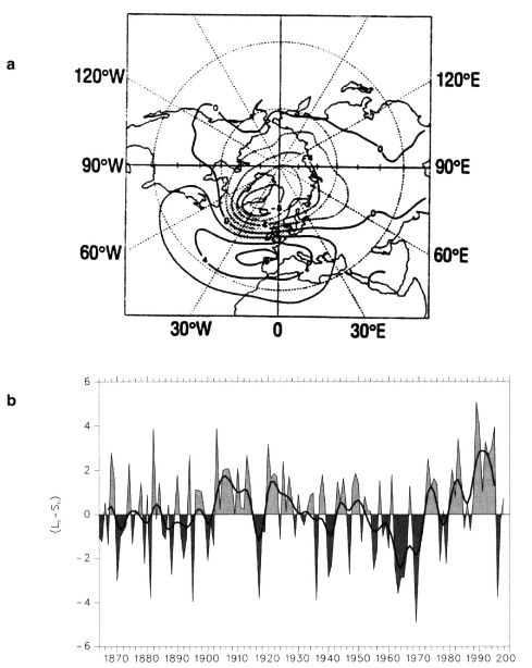
Figure 3-1
(a) Differences between sea-level pressures in high and low NAO-index years, showing the region of
NAO influence. (b) Variation in the NAO (December-March) index since 1864; the heavy line represents
a filtered version of the data. (Both figures from Hurrell, 1995; reprinted with permission of the American
Association for the Advancement of Science.)
Page 27
when the index is high the Icelandic low is strong, which increases the influence of cold Arctic air masses on the northeastern seaboard of North America and enhances the westerlies carrying warmer, moister air masses into western Europe in winter (Hurrell, 1995). Thus, NAO anomalies are related to downstream wintertime temperature and precipitation across Europe, Russia, and Siberia (Hurrell and van Loon, 1996; Hurrell, 1995). They have also been linked (see, e.g., Dickson et al., 1996) to changes in the thermohaline circulation in the North Atlantic (Lazier, 1988), the cod stock in the northwest Atlantic Ocean (Dickson et al., 1988), the mass balance of European glaciers (Pohjola and Rogers, 1997), the Indian monsoon (Dugam et al., 1997), and the atmospheric export of North African dust (Moulin et al., 1997).
Pacific-North American Pattern
The Pacific-North American (PNA) pattern represents a large-scale atmospheric teleconnection between the North Pacific Ocean and North America. It appears as four distinct cells in the 500 hPa (hPa are equivalent to mb) geopotential height field near Hawaii, over the North Pacific, over Alberta in Canada, and over the Gulf Coast of the United States. Wallace and Gutzler (1981) defined an index for the phase of this teleconnection pattern through a weighted average of 500 hPa normalized-height anomaly differences between the centers of the four cells. (Figure 3-2a shows the region and extremes of influence of the PNA pattern, and Figure 3-2b shows 15 years of variation in the PNA index.) The PNA is reflected in SLP (Rogers, 1990) as well, however, and can
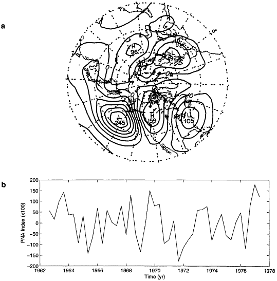
Figure 3-2
(a) Composite of the difference in the 500 hPa height field associated with the ten extreme positive and ten extreme
negative values of the PNA index for 1962-1977. (b) Time series of the monthly mean value of the PNA index. Only
Dec.-Jan.-Feb. values are shown, with the year tick marks at the Jan. values. (Both figures from Wallace and Gutzler,
1981; reprinted with permission of the American Meteorological Society.)
Page 28
be depicted by the North Pacific Index (NPI) (Trenberth, 1990). The NPI is defined as the averaged SLP over a large area of the North Pacific Ocean near the center of the Aleutian low.
It has been speculated that the decadal variability of the PNA and NPI is associated with decadal changes in the tropical Pacific, as discussed below (Nitta and Yamada, 1989; Graham, 1994; Lau and Nath, 1996). Interdecadal variability of ENSO (discussed below in the section on the role of dec-cen variability in global warming) and the PNA is also thought to be responsible for a significant amount of the variance in the salmon inventory along the northwest coast of North America (Mantua et al., 1997).
Other Patterns of Interest
Regional Patterns
The NAO and PNA patterns introduced above, while predominant in the literature and displaying variability on decadal time scales, represent but two of those identified. A number of other regional atmospheric or SST patterns have been analyzed, such as the North Pacific Oscillation (NPO) (Walker and Bliss, 1932; Rogers, 1981), West Pacific Oscillation, West Atlantic Pattern (Wallace and Gutzler, 1981), and Pacific Decadal Oscillation (Mantua et al., 1997). Other atmospheric patterns, such as the Pacific South American pattern, have been identified in the Southern Hemisphere; the data are frequently too sparse in time and space to allow more detailed analyses of these patterns, however. In addition, other structures exist that may or may not be considered climate patterns, although they are often related to the other patterns or presented in a similar manner. For example, the Asian monsoon, while predominantly a seasonal signal, is strongly correlated with ENSO and shows decadal variability as indexed by precipitation and wind speeds over India. Some investigators treat it as another distinct form of decadally varying pattern.
The number of regional patterns identified in the Northern Hemisphere is on the order of 10 (Wallace and Gutzler, 1981; Esbensen, 1984; Barnston and Livezey, 1987), which raises a question as to whether they are all unique. If atmospheric variability amounted to a continuum (i.e., no phase preference existed, a situation comparable to "white noise" in the frequency domain), then statistical analyses, such as those used in teleconnection studies, would produce a finite number of teleconnections (see, e.g., Wallace, 1996). Thus it has been suggested that the multiplicity of patterns is partially the result of a regional continuum (Kushnir and Wallace, 1989; Wallace, 1996), and that not all teleconnections are indeed unique phenomena.
Cold Ocean-Warm Land
Finally, one other "pattern" warrants introduction here. This is the "cold ocean-warm land" or COWL pattern (Wallace et al., 1995). The COWL pattern is not a fundamental mode of climate variability as defined through the decomposition of climatological variable fields, nor is it a particular climate phenomenon; rather, it simply represents a distinct geographic distribution of near-surface temperature anomalies predominantly reflecting the contrast in thermal inertia between land and ocean (Wallace et al., 1995, Broccoli et al., in press). In particular, the COWL pattern is a Northern Hemisphere winter phenomenon that is a manifestation of the dominant effect of the continental land masses on the mean surface air temperature during the cold season. It shows considerable high-frequency variability (e.g., monthly), because the air over the ocean responds slowly to change because the ocean's large heat capacity makes it slow to change, whereas the response of air over land is considerably faster because the land's small heat capacity permits more rapid response. These differences lead to rapid change over land in concert with large-scale shifts in the atmospheric circulation cells, while change over the oceans is much slower and more attenuated. Despite the apparent short-term memory of the COWL pattern, it displays long-term variability as well, which is of particular importance to the global warming experienced over the last 20 years. The lower-frequency variability of the COWL pattern seems to be related to long periods of simultaneous surface warmth in northwestern North America and the Eurasian continent, and can be identified with the simultaneous phase-locking of the PNA and NAO patterns (Wallace et al., 1995; Hurrell, 1996).
Co-Variability in the Climate System: Coupled Patterns
Coupled patterns have expressions in at least two climate-system components, but they are not presumed to be causally related. The term therefore includes coupled modes, but also refers to patterns in each component that are simply coherent.
Tropical Atlantic Variability
Numerous studies have found a robust relationship between SST anomalies in the tropical Atlantic and changes in soil moisture, albedo, and surface-roughness over North Africa (see Nicholson, 1989, for a brief overview). SST anomalies appear to be responsible for a large part of the variability in tropical rainfall over Africa and Brazil. Observational studies by Hastenrath and Heller (1977) and Lamb (1978) were the first studies that linked the variability in tropical Atlantic SST to variability in the rainfall over the Sahel and Nordeste Brazil, respectively (see also Markham and McLain, 1977; Lamb et al., 1986; Hastenrath and Greischar, 1993; Rao et al., 1993). (Figure 3-3 illustrates the correlation between tropical Atlantic convection and Nordeste Bra-
Page 29
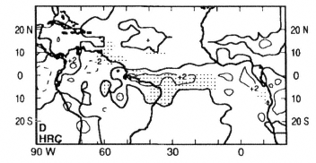
Figure 3-3
March-April field of convective activity in the tropical Atlantic sector.
Shown are the differences in the number of days per month with highly
reflective clouds for Nordeste Brazil wet (1984-1986, 1989) minus dry
(1980, 1982, 1983, 1990) years. Significance of differences at the 5 percent
level, as determined from t-test, is indicated by dot raster. (From Hastenrath and
Greischar, 1993; reprinted with permission of the American Geophysical Union.)
zil precipitation.) Together these observational studies indicate that rainfall variability is associated with changes in the position and structure of the Intertropical Convergence Zone (ITCZ), a band of surface wind convergence characterized by strong and frequent convective activity, which in turn is extremely sensitive to variations in the meridional SST gradient. (See also Lamb, 1978; Shinoda, 1990; Rowell et al., 1992; and Nobre and Shukla, 1996, for discussion of this topic.) Similarly, atmospheric general-circulation model (GCM) studies using prescribed SST anomalies also show the importance of tropical SST anomalies in generating and controlling rainfall anomalies in Brazil and Africa (Moura and Shukla, 1981; Mechoso et al., 1990; Hastenrath and Druyan, 1993; Folland et al., 1986; Owen and Folland, 1988; Palmer et al., 1992; Rowell et al., 1992; Semazzi et al., 1993).
The tropical Atlantic Ocean shows a coherent structure in SST variability. The dominant pattern of SST, as defined by empirical orthogonal function (EOF) analysis, often shows a warm pool in the tropical North Atlantic and a complementary cool pool in the tropical South Atlantic, or vice versa. These centers of action seem to vary coherently over decadal time scales but independently on shorter time scales (Houghton and Tourre, 1992; Mehta and Delworth, 1995; Chang et al., 1997). Consequently, this phenomenon is sometimes referred to as the Atlantic Tropical Dipole, although the lack of a clear consensus on the actual dipole nature of the pattern leaves many simply referring to it as the decadal tropical Atlantic SST variability. This low-frequency SST phenomenon shows concurrent anomalies in the rainfall over Brazil and northern Africa (Figure 3-4a). Periods of greater-than-normal rainfall were experienced over northeast Brazil in the 1960s, and periods of lower-than-normal rainfall in the mid-1970s to early 1980s (Figure 3-4b). Gray (1990) suggests that the decadal changes in the SST in the subtropical North Atlantic may also be responsible for the changes in the distribution and intensity of hurricanes in this region.
While the physics of the dipole climate oscillations in the
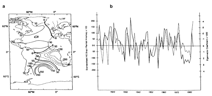
Figure 3-4
(a) The spatial pattern of the EOF of Atlantic SST that is strongly related to rainfall in Nordeste Brazil and western Africa. (b) Time series
(solid line) of the March-to-May values of the EOF shown in (a) and the north Nordeste Brazil rainfall anomalies (dashed line). (From Ward
and Folland, 1991; reprinted with permission of John Wiley and Sons, Ltd.)
Page 30
tropical Atlantic are not yet understood, recent results from Chang et al. (1997) demonstrate that an intermediate-level coupled atmosphere-ocean model of the tropical Atlantic does support decadal oscillations that have a structure similar to the observed dipole phenomenon. Finally, the climate in and around the Atlantic is also affected by variability in the tropical Pacific on both the interannual (see, e.g., Folland et al, 1986; Hastenrath et al, 1987; Enfield and Mayer, 1997) and decadal (Zhang et al., 1997) time scales.
As in the tropical Pacific, within 5º of the equator (the so-called tropical waveguide), ocean dynamics seem to play a significant role in the generation of SST anomalies on the interannual time scale and in the equatorial waveguide (Zebiak, 1993). The SST anomalies in the waveguide are linked to interannual variations in rainfall along the Guinea coast (Wagner and da Silva, 1994). However, little is known about the cause of the low-frequency variability in the SST of the tropical and subtropical Atlantic that is associated with the large-scale rainfall anomalies and with the variations in hurricane activity.
North Atlantic Variability
Kushnir (1994) examined the multidecadal variability in the observational record of SLP, SST, and surface wind velocity in the North Atlantic basin, and found two examples of warm and cold epochs in the twentieth century; each of these epochs lasted more than a decade. Warm periods are characterized by positive SST anomalies around southern Greenland and negative anomalies along the northeastern U.S. seaboard (upper panel of Figure 3-5). The concurrent SLP and wind anomalies indicate a southern displacement of the Icelandic low and a relaxation of the winds in the subtropics (lower panel of Figure 3-5) coinciding with a decrease in NAO. Kushnir (1994) concluded that the variability demonstrated on these time scales in the observational record was governed by a basin-scale interaction between the large-scale oceanic circulation and the atmosphere.
Deser and Blackmon (1993) found that SST in the North Atlantic subpolar basin varied concurrently with the atmospheric surface wind anomalies. These atmosphere and ocean anomalies span the twentieth-century record and display a roughly 10-year period. Deser and Blackmon also note that the spatial relationship between SST and wind anomalies in these quasi-decadal cycles is consistent with what could be expected theoretically if the phenomenon were inherently due to coupling between the atmosphere and the ocean. They point out, however, that there is a high negative correlation between the SST anomalies and the anomalies in sea-ice extent in the Baffin Bay/Labrador Sea region. Furthermore, the sea-ice anomalies lead the SST and wind anomalies by a few years.
In addition to the above phenomena, an event that began in the late 1960s has drawn unusual attention from the ocean community. A significant surface freshwater anomaly ap-
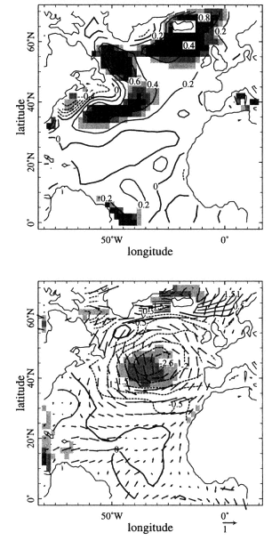
Figure 3-5
Upper panel: The difference between the annual winter Atlantic SST
averaged from 1950-1964 (warm years) minus the winter average from
1970-1984 (cold years). Contour interval is 0.2ºC. Lower panel: as above,
but for SLP and winds. Contour interval is 0.5 mb. The arrow at the
bottom of the panel is 1 m s-1. Distribution of the t-variable corresponding
to SST and SLP differences is denoted in three levels of gray: light for 2.0-
2.5, medium for 2.5-3.0, and dark for 3.0-3.5. (From Kushnir, 1994; reprinted
with permission of the American Meteorological Society.)
peared in about 1969 in the Labrador Sea. Now known as the "Great Salinity Anomaly" (GSA), this feature can be traced moving eastward across the subpolar gyre, into the Norwegian Sea, and ending up near Fram Strait more than 10 years later (Dickson et al., 1988). Aagaard and Carmack (1989) hypothesize that the GSA was born from an increase
Page 31
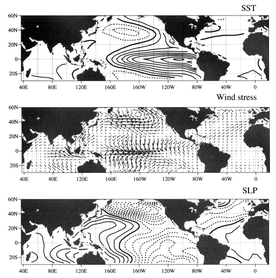
Figure 3-6
Global SST pattern, wind stress, and sea-level pressure that is related to the interannual variability associated with ENSO,
based on linear regression between a high-pass-filtered "cold-tongue index" (CT) and global SST. (From Zhang et al.,
1997; reprinted with permission of the American Meteorological Society.)
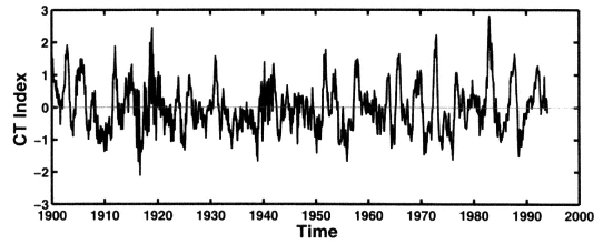
Figure 3-7
Time series of a cold-tongue index, corresponding to the SST pattern displayed in Figure 3-6.
(From Zhang et al., 1997; reprinted with permission of the American Meteorological Society.)
Page 32
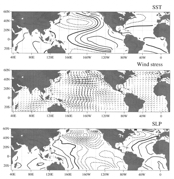
Figure 3-8
Global residual (GR) SST pattern, wind stress, and sea-level pressure, from which the linearly related ENSO
variability has been removed. (From Zhang et al., 1997; reprinted with permission of the American Meteorological Society.)
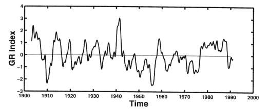
Figure 3-9
Time series of the global-residual index, corresponding to the SST pattern displayed in Figure 3-8,
which indicates that the ENSO-like pattern in that figure is associated primarily with decade-to-
century-scale variability. (From Zhang et al., 1997; reprinted with permission of the American
Meteorological Society.)
Page 33
in sea-ice export from the Arctic (see also Hakkinen, 1993, and a related paper by Mysak et al., 1990). There is evidence that the GSA's stabilization of the upper water column interrupted deep-water production in the North Atlantic (Lazier, 1988). Thus, the GSA is thought to be an example of phenomena that may lead to changes in the thermohaline circulation in the ocean, which may then lead to feedbacks to the atmosphere on much longer time scales.
Pacific Decadal Enso-like Pattern
Tanimoto et al. (1993) and Zhang et al. (1997) demonstrate that the time variability of the leading EOF of the global SST field is separated into two components: one identified with ENSO variability (Figure 3-6) showing predominantly interannual variability (Figure 3-7), and the other a linearly independent "residual" (Figure 3-8) dominated by dec-cen-scale variability (Figure 3-9). The two components exhibit remarkably similar spatial signatures in global SST, SLP, and wind-stress fields, with the SST field in the residual pattern being less equatorially confined in the eastern Pacific than the interannual pattern, and having a larger extratropical signature in the North Pacific. In fact, the residual pattern is very similar to the leading EOF of North Pacific SST that Mantua et al. (1997) have called the Pacific (inter)Decadal Oscillation (PDO). The residual pattern's SLP signature is also stronger in the extratropical North Pacific, and its wintertime 500 hPa height anomaly (Figure 3-10) more closely resembles the PNA pattern than the ENSO pattern shown in Figure 3-6. The amplitude time series of the ENSO-like pattern in the residual variability reflects much of the low-frequency variance in the data as well as some of the interannual variability, including a notable regime shift in 1976-1977 (Quinn and Neal, 1984) and an equally remarkable shift of polarity in the 1940s (see Figure 3-9).
This ENSO-like pattern in SST appears to be teleconnected to anomalies in the mid-latitude atmosphere and ocean of the North Pacific (Figure 3-6). The decadal ENSO-like anomalies of Figure 3-8 are also teleconnected throughout the tropics, with large concurrent changes in tropical Atlantic and Indian Ocean SST (Zhang et al., 1997), as well as the North Pacific (see, e.g., Kumar et al., 1994). Unlike the previous patterns, which are clearly defined through EOF analyses of atmospheric or ocean property fields, this pattern appears only when the data (atmosphere or ocean fields) are time-filtered prior to the analysis. However, because of its large spatial influence and its apparent relationship to the shorter-time-scale ENSO phenomenon, it has received considerable attention in recent years.
The last few decades have represented a warm phase of this climate anomaly, which has preceded a significant reduction in the alpine glaciers throughout the tropics (Thompson et al., 1993b; Diaz and Graham, 1996). In addition, the streamflow and snowpack in the northwest and southwest of North America (Cayan and Peterson, 1989; Cayan, 1996) are well correlated with this time series of the decadal ENSO-like climate phenomenon.
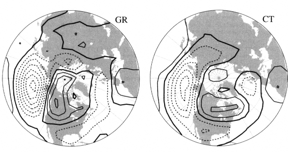
Figure 3-10
The 500 hPa height anomalies associated with the cold-tongue index (CT) (right panel), characterized by interannual
ENSO variability, and the global-residual index (GR) (left panel), characterized by ENSO-like decadal variability.
(From Zhang et al., 1997; reprinted with permission of the American Meteorological Society.)
Page 34
Pacific Summer Variability
Norris and Leovy (1994) point out that there are long-term trends in summer SST in the North Pacific over the period 1952-1981, and that the changes in SST are significantly anti-correlated with the long-term trends in the maritime stratiform cloudiness. They note that the strongest (anti)correlations between SST and maritime stratiform cloudiness are found co-located with the largest climatological SST gradients. Norris and Leovy suggest that these trends may result in part from the persistence of SST anomalies from winter to summer.
Arctic Variability
When Walsh et al. (1996) examined the long-term record of SLP in the Arctic basin, they found that a large decrease in the annual mean SLP occurred in the mid-to-late 1980s. The anomalously low SLP persisted through 1994, the end of the record they examined. The SLP anomalies are largest in the central Arctic, decreasing toward the adjacent coastal regions around the Arctic Ocean; they are present year-round but are greatest in the winter season. The annual mean pressure changes are larger there than anywhere else in the North-em Hemisphere.
Walsh et al. argue that it is unlikely that the observed change in the Arctic atmospheric circulation could be associated with low-frequency variability in the extrapolar regions. They note, however, that the observed changes in the atmospheric circulation can be expected to lead to changes in the transport and compactness of the sea ice in the Arctic basin. Specifically, the mean anticyclonic motion of the ice pack should decrease, and the sea ice should now be more divergent than it was during the 1970s and early 1980s. Indeed, there have been two remarkable large-scale anomalies in Arctic sea ice in the past decade: the extraordinarily thin sea ice that was experienced by the SHEBA (Surface Heat Budget of the Arctic project; see Moritz and Perovich, 1996, for a description) in the winter of 1997 (McPhee et al., 1998), and the offshore contraction of the sea ice off Siberia in 1990. The latter, which is unprecedented in the record, has recently been linked to changes in the pan-arctic atmospheric circulation (specifically, the wind stress) by Serreze et al. (1995) and Bitz (1997). Cavilieri et al. (1997) note that the areal extent of sea ice has decreased by about 6 percent between 1978 and 1996.
The large trends in the Arctic atmospheric circulation and in the NAO (see, e.g., Figure 3-1) during the past 30 years appear to be related (see Thompson and Wallace, 1998, and references therein). Thompson and Wallace argue that these large-scale decadal trends are best described in terms of a planetary-scale mode of variability, which they referred to as the Arctic Oscillation (AO), whose regional extension into the North Atlantic accounts for the phenomena attributed to the NAO. The AO involves fluctuations in the strength of the polar vortex that extend from the surface upward into the lower stratosphere, and occur on time scales ranging from weeks to decades. The ''high index'' (strong westerlies) polarity of the AO is characterized by mild wintertime temperatures over most of Eurasia poleward of 40ºN. Stratospheric involvement in the AO is most clearly apparent during late winter and early spring, when wave-mean-flow interactions at these levels are strongest. Thus, the trend in the AO, and hence in the NAO and Arctic circulation, may be viewed as a systematic bias in one of the atmosphere's most prominent modes of internal dynamic variability. Whether it is occurring in response to anthropogenic forcing has yet to be determined.
Thompson and Wallace (1998) found that the AO, as represented by the first empirical orthogonal function (EOF) of SLP, changed rapidly in amplitude during the mid- to late 1980s. This change is consistent in timing and sense with the changes noted by Walsh et al. (1996). Furthermore, this atmospheric change coincides with a number of additional changes noted in the sea ice and upper ocean. (The precise timing of the changes is unknown for most of the upper-ocean variables, given the relatively sparse data available for the Arctic region.) For example, data collected through the early 1990s by Morison et al. (1998), Carmack et al. (1995, in press), McLaughlin et al. (1996), and Steele and Boyd (in press) all show that the position of the central Arctic upper-ocean front, which separates the Atlantic and Pacific waters, has shifted relative to the 1950-1989 climatological position (as established using the Environmental Working Group atlas built from U.S. and Russian hydrographic observations released through the Gore-Chernomyrdin joint commission); the region dominated by Atlantic water has expanded by nearly 20 percent. These same data, as well as those of Anderson et al. (1994), Rudels et al. (1994), and Quadfasel (1991) suggest a warming of the Atlantic layer occurring at this same time. Other studies are finding changes in the surface winds, sea ice, and other upper-ocean characteristics, such as pycnocline properties. Four summers with the most extreme minimum Arctic sea-ice coverage (Maslanik et al., 1996) have occurred since this change took place, and anomalously thin ice has also been reported (McPhee et al., 1998). Together, these ocean, ice, and atmosphere observations suggest that the changes in the late 1980s in the Arctic may have involved the entire vertical column from the upper ocean to the stratosphere.
There are, however, theoretical reasons to expect large variability in Arctic systems because of the coupling among the polar atmosphere, ocean, and sea ice. First, the Arctic sea-ice thickness is thought to be extremely sensitive to changes in vertical heat transport in the ocean (see, e.g., Maykut and Untersteiner, 1971); only modest circulation changes in the ocean would be required to induce variability in the ocean heat transport that would have a significant impact on the thickness and spatial extent of the Arctic sea ice,
Page 35
and hence on the albedo of the Arctic. In addition, it has recently been argued that the observed high-frequency (subseasonal) variability in atmospheric energy transport into the Arctic may lead to large variability in Arctic sea-ice thickness in the Arctic that occurs primarily on decadal and multidecadal time scales (Bitz et al., 1996).
Variability of the sea ice in the Arctic is a defining aspect of the Arctic climate system. In addition, the ramifications of changes in Arctic circulation and sea ice are clearly important for understanding the circulation of the subpolar North Atlantic Ocean mentioned earlier. Thus, while the connections between the AO and NAO, and the polar and extra-polar regions, are still unclear, their co-variability suggests that these coupled Arctic variations are intimately tied to extra-polar regions.
Antarctic Variability
A completely different kind of pattern involving sea ice, surface winds, SST, and SLP has been found in the Southern Ocean. Specifically, the Antarctic Circumpolar Wave (ACW) is characterized by co-varying deviations in monthly climatological averages of these variables along the Antarctic polar front, near the winter marginal ice zone (White and Peterson, 1996). It is also highly coherent with temporal variations in ENSO (White and Peterson, 1996) and the Indian Ocean monsoons (Yuan et al., 1996), although the underlying physics are not yet understood. It is predominantly an interannual phenomenon, but, as with ENSO, it shows longer-period variability. It is not clear how the ACW is related to, or interacts with, the dominant mode of variability of the zonal mean flow in the Southern Hemisphere (Hartmann and Lo, 1998), or the standing-wave patterns of van Loon and Jenne (1972) and van Loon et al. (1973), though the superposition of these various patterns in space suggests that their interaction is feasible.
The Role of Dec-Cen Variability in Global Warming
It is clear that the global warming experienced over the past 20 years is distinguished by an enhanced warming in winter that was not evident in previous decades, dominated by a strong warming over Northern Hemisphere land, and compensated for to some degree by a lesser cooling over parts of the Northern Hemisphere oceans. Despite its decadal persistence, this pattern is consistent with the basic COWL pattern described above. Its geographic aspect is readily apparent in the global surface-temperature data when the last 20 years are compared to the previous 20 years (Color plate 1). A pattern similar to the COWL pattern (though not identified as the COWL pattern) is produced by numerous modeling studies simulating anthropogenic inputs, and thus is considered by some to be one component (of several) of the so-called "greenhouse fingerprints" (Wigley and Barnett, 1990; Santer et al., 1995). Its presence in the actual observational data has therefore been accepted as additional evidence of anthropogenic warming (IPCC, 1996a).
Figure 3-11 shows that when the monthly-average Northern Hemisphere surface-temperature time series for this century is adjusted to eliminate the influence of the COWL pattern, two things become apparent (Wallace et al., 1995): (1) a large fraction of the month-to-month variability, which is particularly apparent in the colder half of the year, is removed; and (2) a significant fraction of the accelerated warming in the cold-season months that has been apparent since the mid-1970s (Figure 3-11, middle panel) is also removed, and the summer and winter trends become comparable (bottom set of curves).
Further investigation suggests that much, though not all, of the accelerated warming that has occurred since the mid-1970s is attributable to the COWL pattern. Much of the COWL pattern itself can be explained by the synchronous polarity of the NAO and PNA patterns during this accelerated period of warming (Hurrell, 1996). That is, over the
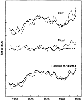
Figure 3-11
Top, smoothed monthly-average surface-temperature time series for the Northern Hemisphere.
The solid line is the warming-months average, the dashed line the cooling-months average.
Center, the portion of the series attributed to the COWL pattern. Bottom, the time series adjusted
by eliminating the COWL contribution. (From Wallace et al., 1995; reprinted with permission of the
American
Association for the Advancement of Science.)
Page 36
last 20 years, the NAO and PNA patterns (the latter represented by the North Pacific Index) both seem to show a seemingly unusual persistent tendency, on average, to occupy states that favor a warming of Europe and Northern Asia by the NAO, and warming of North America by the PNA. When this warming is removed, the global warming trend of the last 25 years is similar to, though slightly larger than, the warming that occurred over several decades in the early part of this century (from 1910 to 1940, say). Broccoli et al. (in press) find that their coupled model reproduces this warming attributed to the COWL pattern. They also find that such an accelerated warming is highly anomalous (exceeding the 99th percentile) in simulations that do not contain greenhouse warming. The extent to which the COWL pattern is anthropogenically caused or influenced is an outstanding issue, and one crucial to all aspects of the greenhouse-warming puzzle.
Another critical question is whether anthropogenic increases in radiative forcing play a role in amplifying the intensity, frequency, and/or duration of ENSO events. For example, several works have shown that the coupled ocean-atmosphere system, particularly in the tropical Pacific Ocean, plays an important role in regulating the mean climatological state (see, e.g., Neelin and Dijkstra, 1995; Sun and Liu, 1996; Clement et al., 1996; Seager and Murtugudde, 1997; and Cane et al., 1997). Sun and Trenberth (1998) extend this concept by suggesting, on the basis of an observational study, that the E1 Niño events are an effective means for removing heat from the tropical Pacific and may even arise as a necessity for removing excess heat associated with increased solar heating and the greenhouse effect. This suggestion is also consistent with a number of coupled-modeling studies of increased radiative forcing or increased CO2 that have shown more energetic and more extreme ENSO events (Sun, 1997; Timmermann et al., 1998; and an ENSO-like pattern of response (see, e.g., Meehl and Washington, 1996, and Knutson and Manabe, 1995, in press). Much of our current uncertainty regarding the role of the coupled ocean-atmosphere system in greenhouse warming is the result of uncertainties involving the role of the cloud-radiative feedback, which underscores the need to improve model representations of this critical process. Substantial uncertainties regarding model response of the tropical Pacific to greenhouse warming also arise in the modeling of the equatorial thermocline.
Such a response has been suggested by Trenberth and Hoar (1995, 1997). Through analyses of more than 100 years of climate data they concluded that the record of the Southern Oscillation Index (SOI) in the period since 1976 is significantly different from the earlier portion of the record. Though this research preceded the powerful 1997-1998 El Niño event, they found a recent tendency for more frequent El Niño events and fewer La Niña events (contrary to the model results of Timmermann et al. (1998)). Although Trenberth and Hoar posit that this change may be caused by the observed increase in greenhouse gases, it is not currently possible to say definitively what underlies this change in character of El Niño events (NRC, 1996). Trenberth and Hoar's conclusions are predicated on a statistically stationary, linear-time-series model of the SOI time series. Rajagopalan et al. (1997) offer an alternative viewpoint using a time-series model whose parameters are allowed to vary slowly over time. This analysis highlights significant dec-cen variability both in the probability of El Niño and La Niña states, and in the probability of transitions between these states. Their results suggest that the recent tendency to more frequent and persistent El Niño events may not be nearly so unusual as Trenberth and Hoar indicate. These differences underscore the need to discriminate better between natural and anthropogenic causes for dec-cen variability, and to think further about what statistical methodology is appropriate for such analyses. By improving our understanding of how anthropogenic climate change interacts with natural processes such as El Niño, we will improve our ability to detect global warming signals, and perhaps gain predictive insight into the dec-cen-scale modulation of phenomena that have traditionally been viewed in a seasonal-to-interannual context.
Finally, it is interesting to note that the analysis of Huang et al. (1998) of 135-year-long indices has revealed a relationship between the NAO, ENSO, and PNA, albeit a complex one. They find that an enhanced positive phase of the PNA is likely to occur with the positive phase of the NAO. Furthermore, at frequencies of 2 to 4 years, the NAO is coherent with ENSO from 1960 to 1990; this coherence is most apparent during strong to moderate El Niño events. (This result is consistent with the findings of Rogers (1984).) As noted earlier, the COWL spatial pattern also correlates with positive NAO and PNA indices. Greenhouse warming thus carries the potential for altering all four patterns. Our understanding of the climate system' s likely response to anthropogenic forcing might benefit from considerable attention to the relationships between greenhouse warming and these (and other) natural modes of variability.
Fundamental Issues and Questions
The patterns and coupled modes occupy large spatial areas, describe significant climate variance, and bridge high-, mid-, and low-latitude zones. Despite the uncertainties about their roles in anthropogenic global warming and natural climate change, they represent an obvious avenue through which coherent climate variations and change may be propagated globally. The IPCC Second Assessment (IPCC, 1996a) noted that much of our attention has recently shifted from the analysis of mean global temperature to that of its spatial distributions, anticipating that climate change might manifest itself irregularly in space and time—yet patterns have appeared. The identification of coherent patterns with coupled modes that explain significant fractions of the spatial and temporal variability offers hope that there may be a
Page 37
signal in what appears to be just "noise." Furthermore, the apparent persistence of these patterns in time, even allowing for a slow evolution, provides additional hope that these signals may be exploited to help us understand and predict future climate variability and change. Also, the apparent relationship between specific climate-pattern dispositions and regional climate characteristics lends support to the notion that understanding long-term trends in the patterns may enable us to make short-term predictions for some regions.
To realize these potentials, considerable effort must also be invested in improving our general understanding of the patterns and coupled modes: their mechanisms (dynamic and thermodynamic, natural and anthropogenic), couplings, feedbacks, and sensitivities. These are truly cross-disciplinary issues, requiring a strong interdisciplinary approach. Specifically, we must answer the following questions:
• What is the longevity of the patterns and their spatial/ temporal variance? The patterns offer tantalizing evidence that some fraction of the Earth's climate shows spatially and temporally coherent structure with some degree of (predictable) persistence in a time-averaged sense. However, the fundamental patterns themselves may be transitory phenomena reflecting the current configuration of a slowly changing climate. Consequently, we need to understand the dynamics between climate patterns and the general state of climate. For example, do the patterns and climate evolve in a systematic manner? At some level of change do the patterns become simple artifacts of the change, as opposed to predictors of the change?
• What is the best way of characterizing the known patterns, and are there additional patterns of interest? Specifically, how can we most effectively define their salient features, their co-varying components and coupled modes (including regional influences and correlation with or control of the climate attributes discussed in Chapter 2), their sensitivities to analysis technique, and their spatial distribution and broader teleconnections? Likewise, robust and optimal indices of these coherent atmospheric-circulation patterns need to be established, because some of the indices employed to represent the patterns, while convenient, do not capture much of their spatial and temporal complexity. For example, the Bermudan-Azorean high remains relatively stable in its spatial orientation, but the Icelandic low often migrates southward to Newfoundland, and the North Atlantic SST pattern tends to show a rotation around the North Atlantic basin (see, e.g., Hansen and Bezdek, 1996) that a simple dipole index, such as the NAO, relating two fixed points, cannot capture. The new findings of Thompson and Wallace (1998), showing that the first EOF of Arctic SLP may be an even better indicator of Eurasian climate change than the NAO, further underscores the need to examine the optimal means of classifying the relevant modes of climate. Therefore, while indices have proven useful in their ability to simplify the temporal history of complex patterns and demonstrate their broad spatial coherence and importance, additional research is required to better characterize the patterns and isolate their significant characteristics. That is, more robust indices that efficiently describe the fundamentally important characteristics of the patterns must be developed. What patterns and coupled modes exist in data-poor regions, and what are their spatial and temporal characteristics?
• Which patterns represent true dynamic modes, and which ones are simply statistically consistent structures, or geographically forced distributions? That is, are the patterns fundamental modes of climate variability reflecting coupled, internal, and external dynamics and thermodynamics? Or are they simply the reflection of structures that are intrinsic to the atmosphere (i.e., determined by the land-sea distribution and internal atmospheric dynamics)? In the latter case, they stochastically force the ocean (see, e.g., Hasselmann, 1976), integrate the response, and provide a feedback to the atmosphere by "reddening" the spectrum of the patterns in the atmosphere without affecting atmospheric dynamics (Barsugli and Battisti, 1998). Or are they the consequence of statistics or chaos, representing attractors of random but spatially consistent distributions? Understanding the mechanisms underlying these patterns will be fundamental in our assessment of how they can ultimately be used in long-term forecasting and prediction of climate variability and change.
• What are the mechanisms responsible for generating, maintaining, and modifying the patterns? What role do these mechanisms play in the spatial propagation of regionally initiated variability or change, and what are their critical dependencies ? To understand how a change in the state of a pattern in one location may dictate the regional climate in some more remote location, it is necessary to understand the mechanisms that control the spatial and temporal evolution of the patterns and their broader influences or teleconnections. This knowledge will also provide an indication of how a local disturbance may influence the dominant regional pattern, leading to broader propagation of the anomaly, and thus influencing the controlling components of the climate system.
• What is the relationship between decadal-to-centennial patterns and global warming? What part of the COWL warming pattern is due to natural variability versus anthropogenic modulation of these naturally occurring patterns? Will there be extended periods of time in which they display similar, relatively persistent polarity quite by chance, or is COWL a manifestation of anthropogenic warming through the polarity of the natural climate modes? (See discussions by Wallace et al. (1995) and Hurrell (1996).) Is the residual warming—that is, warming apart from the COWL contribution—natural variability or anthropogenic warming? What is the relationship between the COWL pattern, greenhouse fingerprint, and natural climate patterns—that is, how do the natural modes of the climate system respond to different changes in forcing, natural or anthropogenic? Are there unique characteristics or
Page 38
response modes? What controls the degree and nature of the spatial distributions and interactions of the modes, and how do they co-vary?
It is clear that a more comprehensive understanding of the variability of these patterns on decade-to-century time scales is absolutely essential if we are truly to distinguish between anthropogenic change and natural climate variability, or understand their interaction. If an enhanced greenhouse effect strengthens or phase locks existing natural modes of variability, the study of dec-cen variability and the study of anthropogenic change are inextricably combined. It will be impossible to understand one without the other.


