(NAS Colloquium) The Age of the Universe, Dark Matter, and Structure Formation (1998)

Proc. Natl. Acad. Sci. USA

Vol. 95, pp. 29–34, January 1998

Colloquium Paper

This paper was presented at the colloquium entitled “The Age of the Universe, Dark Matter, and Structure Formation,” organized by David N.Schramm, held March 21–23, 1997, sponsored by the National Academy of Sciences at the Beckman Center in Irvine, CA.

DAVID WILKINSON

Joseph Henry Laboratories. Princeton University, Princeton. NJ 08544

ABSTRACT Most cosmologists now believe that we live in an evolving universe that has been expanding and cooling since its origin about 15 billion years ago. Strong evidence for this standard cosmological model comes from studies of the cosmic microwave background radiation (CMBR), the remnant heat from the initial fireball. The CMBR spectrum is blackbody, as predicted from the hot Big Bang model before the discovery of the remnant radiation in 1964. In 1992 the cosmic background explorer (COBE) satellite finally detected the anisotropy of the radiation—fingerprints left by tiny temperature fluctuations in the initial bang. Careful design of the COBE satellite, and a bit of luck, allowed the 30 µK fluctuations in the CMBR temperature (2.73 K) to be pulled out of instrument noise and spurious foreground emissions. Further advances in detector technology and experiment design are allowing current CMBR experiments to search for predicted features in the anisotropy power spectrum at angular scales of 1° and smaller. If they exist, these features were formed at an important epoch in the evolution of the universe—the decoupling of matter and radiation at a temperature of about 4,000 K and a time about 300,000 years after the bang. CMBR anisotropy measurements probe directly some detailed physics of the early universe. Also, parameters of the cosmological model can be measured because the anisotropy power spectrum depends on constituent densities and the horizon scale at a known cosmological epoch. As sophisticated experiments on the ground and on balloons pursue these measurements, two CMBR anisotropy satellite missions are being prepared for launch early in the next century.

In the standard hot Big Bang cosmological model, cosmic microwave background radiation (CMBR) is the remnant thermal radiation which dominated the development of the very early universe. Its currently observed properties give us an important means of testing the standard model and of studying physical processes in the universe beyond the reach of our most powerful optical telescopes. Measurements by the cosmic background explorer (COBE) satellite show that the CMBR spectrum between wavelengths of 5 mm and 0.5 mm is the same as that of a blackbody emitter with an accuracy of ±0.01% (1), in surprisingly good agreement with predictions based on the hot Big Bang model. Of secondary interest to cosmology, the CMBR temperature is measured as 2.728± 0.004 K. The absence of spectral distortions in the CMBR imposes limits on energy-producing processes in the universe from an age of t˜1 year to an age of t˜10⁸ years. Another critical test of the standard model is to measure and characterize the CMBR anisotropies expected from density perturbations at t˜3×10⁵ years, when the matter becomes neutral and decouples from the thermal radiation for the first time. Theorists predicted CMBR anisotropies of about 1 part in 10⁵ (dT˜30 µK), corresponding to the mass density perturbations needed to seed the mass structure seen in the universe today. In 1992 the COBE science team announced a detection of CMBR anisotropy (2, 3) close to the predicted amplitude at angular scales larger than 10°. Regions of this size were not yet connected by light speed at the time of decoupling, so these perturbations must have been imbedded in the original bang. The physical mechanism for generating the density perturbations may be quantum fluctuations in the very early universe, but this has not yet been verified.

Currently most CBMR observations are designed to measure the angular power spectrum of anisotropies with scales of a few degrees and smaller. The standard model predicts a complex series of peaks caused by acoustic oscillations of the recombining plasma during the decoupling process. The measurements will test the model’s ability to describe detailed physics of this critical epoch in cosmic evolution. Also, because the oscillations depend on the density and horizon size at the decoupling epoch, a careful tracing of the power spectrum of the anisotropies might measure several important cosmological parameters.

One of the three experiments aboard the COBE satellite, the differential microwave radiometers (DMR), was designed specifically to look for large-scale anisotropy in the CMBR. Six radiometers at 31, 52, and 90 GHz measured the CMBR temperature difference between 7° (full width at half maximum) spots 60° apart in the sky. Spacecraft rotation and orbital motion caused the radiometers to scan about half of the sky per orbit. However, although launched in November 1989, the COBE/DMR radiometers were vintage 1975. A year of observation was required before their sensitivity was sufficient to distinguish 30 µK CMBR anisotropy from instrument noise. Even then the detection was a statistical result, because the signal to noise ratio in the map pixels was only about 1:1. Three more years of data were required to reach S/N=2, where some real CMBR features can be distinguished in the COBE/ DMR sky map. The 4-year map is shown in Fig. 1.

It is not well known how close the COBE/DMR came to not detecting the CMBR anisotropy. As one might expect, at the 30 µK level there were several systematic effects competing with the CMBR signal. These effects had to be removed or understood before a CMBR anisotropy detection could be assured. This took about 6 months from the time that the COBE science team first suspected that a CMBR signal was present in the data. The largest systematic effect was due to the

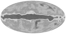
FIG. 1. A map of the CMBR anisotropy as measured by the COBE/DMR radiometers. The temperature range is ±100 µK. A constant level (≈2.73 K) and a dipole distribution have been subtracted to better show the cosmological anisotropies from 10° to 90°. Most of the suppressed dipole is due to the sun’s motion through the reference frame established by the CMBR. The map is in Galactic coordinates, so the Galaxy’s radio emission shows as a bright streak across the middle. Some of the bumps off the Galactic plane are real CMBR anisotropy, some are residual noise.

Earth’s magnetic field affecting the sensitive ferrite switches that alternated the radiometer inputs between two horn antennas pointing 60° apart in the sky. Fortunately, this effect had been seen in balloon-borne experiments using similar radiometer technology, so the switches were magnetically shielded and their susceptibilities measured in preflight testing. Even so, the magnetically induced signal was comparable to the CMBR signal in some radiometers and an empirical correction was needed. Another concern was the magnitude of 300 K Earth emission that diffracted over, or leaked through, COBE’s ground screen. This had not been measured in preflight tests, only estimated from crude (by today’s standards) calculations. The experimental strategy of using several levels of “Dicke” switching caused systematic effects to enter the data stream with different time signatures than that of a sky signal. Switching between antennas at 100 Hz, rotating the spacecraft with a period of 1.25 min, and circling the Earth once every 103 min ensures that systematic effects have a different time signature than that of a true sky signal. For example, the magnetic effect will be largest when mapped in a coordinate system fixed to B_EARTH rather than sky coordinates. For those who worry about such things the most important papers associated with COBE’s anisotropy detection are the ones describing the systematic error analysis (4, 5).

Another concern with the COBE/DMR detection of CMBR anisotropy was the issue of foreground microwave emission from our Galaxy (6, 7). Measurements by radiometers at three different frequencies, all with 7° beams on the sky, were used to separate CMBR anisotropies from foreground emission. The CMBR has a different spectrum from those of known Galactic radiation sources—synchrotron, bremsstrahlung, and 20 K dust emissions. At a level of 30 µK the Galactic emission in the COBE/DMR bands could not be estimated from sky maps at higher and lower frequencies, so the COBE/ DMR data itself had to be used to estimate the Galactic contribution. Fig. 1 clearly shows very bright foreground signals associated with the Galactic plane, but the COBE/ DMR data show that for regions more than 20° from the Galactic plane, the sky fluctuations are dominated by CMBR anisotropies. Luckily, we live in a Galaxy whose microwave brightness is five orders of magnitude weaker than the CMBR radiation at wavelengths near 3 mm. Coincidentally, the peak of the CMBR blackbody spectrum is nearby, at about 2 mm wavelength.

To see the effects of physical processes at the decoupling epoch (age t≈3×10⁵ years, redshift z=1,400), we must measure regions of space that were connected by light speed (causal) at that time. In the standard cosmological model causal events at decoupling are separated by less than about 1° as seen now. Numerical integration of the behavior of matter and radiation through the decoupling epoch have long shown (8) that structure should be expected in the angular power spectrum of anisotropies at scales below a few degrees (9). Recent analytic work on the decoupling process (10) has shown that most of the CMBR anisotropy is caused by acoustic oscillations in the ionized fluid as the universe expands and cools. The scale of the oscillating regions is determined by the speed of sound which in turn is set by the density and composition of the fluid. This is the idea behind using medium-scale anisotropy measurements to test the detailed physics of the cosmological model and, if a model fits the data, to measure the values of some cosmological parameters.

The physics is deceptively simple. During decoupling, as the fluid is still partially ionized, radiation and matter are still coupled, but the coupling is growing weaker as the matter recombines. The acoustical oscillations are caused by mass falling into relatively over-dense regions [caused by clumped dark matter in cold dark matter (CDM) models]. The radiation is compressed like a spring, eventually causing the fluid to rebound and expand. Meanwhile the optical depth of the fluid is decreasing and more and more photons are scattering for the last time. The phase of the fluid oscillation when photons are scattered for the last time determines whether their temperatures will be slightly above or below the mean CMBR temperature. There are several effects that shift the photon frequency, and hence the CMBR temperature. If the photons are scattered for the last time from a compressed region, adiabatic fluctuations imply a higher temperature, but gravitational redshift will cool the CMBR photons as they climb out of the potential wells. If, however, the region is expanding at that time the scattered photons will be blue shifted by the Doppler effect. The gravitational and Doppler effects are 90° out of phase, so they may tend to reinforce or cancel one another. The angular scale of the oscillations that cause CMBR anisotropy is determined by the sound horizon of the fluid at the decoupling epoch. The phase of an oscillation at last scattering is set by its period and the time between when a scale enters the horizon and when the CMBR photon last scatters. Some acoustical oscillation scales release the photons when they are near the extremes of compression or expansion causing these scales to have a larger rms δT than others. Therefore, a measurement of the rms δT vs. angular size—the anisotropy power spectrum—is expected to have peaks from about 1° to 10′.

The detailed shape of the medium-scale anisotropy power spectrum depends on the cosmological model, the constants of that model, and the detailed physics of decoupling. Some predicted peaks are shown in Fig. 2 for various cosmological models of current interest. Accurate measurements of the angular power spectrum can be used to determine the important cosmological parameters of the model (11, 12). For example, the baryon density and Hubble constant, Ω_B and H₀. largely determine the height of the first peak and the ratio between peak heights. The total mass density, Ω₀, and H₀ largely determine the angles at which the peaks occur. Is there, after all. a significant cosmological constant, Λ, in our universe today? Fig. 2 shows that such a model is easily detectable by a well-measured anisotropy power spectrum. A major issue in cosmology research is the whether the universe is open (Ω_TOTAL<1) or closed, perhaps with a large density of unidentified CDM. Finally, what is the nature of those initial perturbations? Are they adiabatic or isocurvature? Again Fig. 2 indicates that accurate measurements of the anisotropy power spectrum can distinguish between these various models. Theoretical cosmologists continue to work out the possible consequences of accurate measurements of the anisotropy

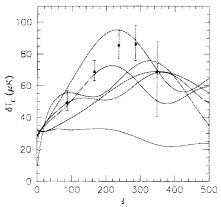
FIG. 2. An illustration of the current situation in medium-scale measurements of the CMBR anisotropy, l is the spherical harmonic index; roughly, angle≈180°/l. These results were obtained from three winter seasons of observations from Saskatoon. SK (22–24). The curves are the CMBR anisotropy predicted by various models, normalized to the COBE measurement at l≈10. From top to bottom at l=160, the models are as follows: CDM, Ω_TOTAL=1, Ω_Λ=0.7: standard CDM; isocurvature; open universe with Ω_TOTAL=0.4; an exotic model where texture seeds structure formation; and a model with postdecoupling re-ionization at a relatively early time. (Figure adapted from ref. 28.)

power spectrum. These simulations are important to experimenters as they try to optimize the designs of new experiments to maximize scientific return. A paper by Bond in this Colloquium (13) presents the theoretical perspective.

There are other physical effects that shape the medium-scale anisotropy power spectrum. The peaks in the power spectrum at small angular scales are attenuated by multiple scattering of photons with large mean-free-path. Similarly, the predicted exponential decay of all anisotropies at small angular scales (≤10′) is due to the smoothing effect of photon diffusion. The scale of the largest oscillating region (a few hundred million light years today) is larger than the thickness of the decoupling shell, but features smaller than the shell thickness are smeared out by photon diffusion. Another anticipated effect is postdecoupling scattering by electrons in a re-ionized intergalactic medium (see the lowest curve in Fig. 2). This re-ionization must come early (z>20) if the electron density is to be high enough to cause significant distortion of the primordial spectrum, as modified by the decoupling processes. Accurate measurements of the power spectrum of medium-scale and small-scale CMBR anisotropy will tell us important details about physical processes occurring in our universe during its first few million years.

After the COBE/DMR detection of large-scale CMBR anisotropy the focus of the field shifted to smaller angular scales. Theoretical work intensified as it became clear that the decoupling epoch could be studied in detail and some important cosmological constants might be measured. Experimenters built larger telescopes to get smaller beams and continued to develop more sensitive detectors and sophisticated observing strategies. Currently, there are three types of detection techniques being used to observe CMBR anisotropies: coherent microwave receivers, low temperature bolometers, and radio interferometers. Detectors are sufficiently difficult to develop that most groups specialize on one or two types. The detector type usually drives the choice of observing frequency, angular scale, and observing platform. Currently, all anisotropy observations are being made from the ground or from balloons; planned observations from satellites will be described in the next section.

Low-temperature bolometers are the most sensitive detectors currently available. Optical techniques can be used to obtain sensitivity to wide frequency bands and many propagating modes, so more energy can be collected from the extended, broadband CMBR source. The disadvantages of bolometeric detectors are their need for relatively complicated cryogenic techniques (T≤300 mK) and the high frequency range needed for best sensitivity, v≥90 GHz. Atmospheric emission is a problem at these frequencies, so observations must be made from the South Pole or mountain tops (14–17) or from balloons (18–22). Foreground emission from Galactic dust competes with the CMBR anisotropy at frequencies >150 GHz, so most experimenters use several frequency bands to measure and remove the dust signal. Coherent microwave receiver techniques use high electron mobility transistor amplifiers (HEMTs) or SIS (superconductor-insulator-superconductor) junction mixers to achieve low instrument noise. HEMT-based receivers are currently limited to frequencies <100 GHz and they have lower sensitivity than bolometers. However, they do not require complex cryogenic systems to give adequate noise performance; they work well at 10 K, which is easily reached by standard mechanical refrigerators. Because the atmosphere is relatively quiet in some bands <90 GHz, HEMT receivers can make good measurements of the CMBR anisotropy from ground-based sites under cold, dry atmosphere (23–25). SIS mixers go higher in frequency, and wide bandwidths can be achieved. They require cooling below 1 K, usually obtained with pumped liquid helium.

Problems due to fluctuations in atmospheric emission can be minimized by making observations from balloons, but observing time is currently limited to about 10 hr per flight. Several groups are working to relax this restriction by developing long duration ballooning techniques—perhaps circumpolar flights of 2 weeks or more. Other groups observe from high altitude sites with particularly dry atmosphere, such as the South Pole, Mauna Kea, or northern Chile. As the accuracy of CMBR anisotropy measurements increases, foreground emission from our Galaxy becomes a more important issue. Measurements at a wide range of frequencies are needed to separate CMBR anisotropies from Galactic radio and dust emission. Because radio emission decreases with frequency, and dust emission increases, there is a minimum in the temperature of foreground emission. The minimum is somewhere between 70 and 90 GHz.

Another way to reduce the effects of atmospheric emission is to use radio interferometer techniques. Interferometers can also achieve higher angular resolution at some sacrifice of sensitivity. The National Radio Astronomy Observatory’s Very Large Array, and the Mullard Observatory’s Cosmic Anisotropy Telescope have already been used to make sensitive measurements of CMBR small-scale anisotropy (26, 27). Because the separate antennas of the array look through different atmospheric paths, most of the atmospheric signal is uncorrelated, whereas the CMBR signal is correlated in all antennas. Currently, observing frequencies are quite low (≤20 GHz) and bandwidths are limited by correlator technology and cost. Of course, the main advantage of interferometer arrays is their capability to measure small-scale anisotropy without having to build a large, expensive mm-wave antenna. Map-making capability is intrinsic to interferometers.

Several dozen measurements of the medium- and small-scale CMBR anisotropy have been made and more are un-

derway in this very active field. Page (28) has compiled a list of properties for recent, current, and planned experiments; a version of that list is shown here in Table 1. As an illustration of the results from a typical experiment, the results from the Saskatoon experiments are shown in Fig. 2. The measured rms anisotropy, dT₁, is plotted against angular scale as represented by the spherical harmonic index, l. A range of angular scales can be studied in these experiments by scanning the beam back and forth across the sky and then doing Fourier analysis of the data. The high l end of the measured spectrum is set by the beam size, and the low l end is set by the length of the scan. Predictions of some cosmological models are also shown in Fig. 2. The re-ionization model seems to be ruled out, but one should treat the results of any single anisotropy experiment with caution. Signals are very weak compared with instrument noise, so the evaluation of systematic effects is difficult. Multiple experiments with different technologies, frequencies, screening, and scanning techniques are needed to assure that it is the true CMBR anisotropy that is being measured.

Fig. 3 shows an attempt by Page (28) to make an objective summary plot of CMBR anisotropy results as of June 1996. He used the compilation of experimental results of Ratra et al. (ref. 29; and B.Ratra, personal communication) and averaged the data into logarithmically spaced angle bins, four per decade. The error bars on dT₁ in each band are derived from the error bars reported by each experimental group. There is a strong indication that the CMBR anisotropy is larger at medium angular scales (100<l<500) than at large scales where the COBE/DMR results anchor the anisotropy at about 30 µK. At small scales upper limits have been set (asterisks in Fig. 3) by interferometer and large single-dish experiments. These indicate a decrease in the small-scale anisotropy spectrum compared with the measurements at medium scales. Perhaps we are seeing the decay of anisotropy expected from multiple scattering of photons at decoupling. However, most experimenters urge caution in the interpretation of current anisotropy results. Only a few measurements have been confirmed by a second group observing the same region of sky (Far Infrared Survey confirms COBE/DMR, see ref. 30; and Saskatoon confirms Medium-scale Anisotropy Measurement, see ref. 31). Calibration and systematic errors are known to be present. Ground- and balloon-based experiments will continue

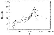
FIG. 3. A graphical summary of experimental attempts (up to June 1996) to measure the medium-scale CMBR anisotropy. Points for l= 17 are from the COBE/DMR experiment; 20<l<800 are the combined (28) measurements of many groups; the asterisks are upper limits from small-scale measurements. The upper and lower curves are estimated one standard deviation error bars for the combined data.

to improve as technology and techniques are developed further. It is very likely that the first peaks in the predicted anisotropy power spectrum will be experimentally checked before either of two planned CMBR anisotropy satellites produce data.

There are two promising innovations underway in this field. Prospects are good for a detection of CMBR polarization, and space missions promise sensitive full-sky measurements of the medium-scale anisotropy. Thirty years ago Rees (32) predicted that the CMBR would be polarized at a level of about 10% of the expected temperature anisotropy—i.e., a polarization signal of a few µK. The polarization is produced at the time of last scattering of CMBR photons. If the scattering electron is bathed by an anisotropic flux of photons in the plane perpendicular to our line of sight, the scattered CMBR that we measure will be polarized. However, because the effect is expected to be much weaker than the temperature anisotropy, instrument sensitivity and systematic errors have so far precluded measurements from reaching the expected levels of a polarization signal. Radiometer sensitivity has now improved to the point where experiments can be designed with an expectation of seeing the CMBR signal (polarization experiments are underway at Wisconsin: University of California, Santa Barbara; Caltech; and Princeton). Also, recent theoretical work has stimulated experimental work by showing that polarization measurements provide new information beyond what can be learned from temperature anisotropy maps (33, 34). For example, postdecoupling re-ionization effects have distinctive signatures in polarization maps, as do tensor perturbations (e.g., due to gravitational waves) in the early universe.

While the COBE satellite was still taking data the CMBR community was beginning to discuss a space mission to make medium-scale CMBR anisotropy measurements.^† Full-sky maps of the sensitivity and angular resolution needed to realize the full scientific potential of the anisotropy signal are best done from space. The COBE satellite had demonstrated the many advantages of using experiments in space to make highly accurate sky maps with relatively noisy and environmentally sensitive instruments. In the spring of 1996 NASA chose the microwave anisotropy probe (MAP) to be one of its first two mid-sized explorer (MIDEX) missions (MAP Web site: http://map.gsfc.nasa.gov/html/tech_overview.html). A few months later, the European Space Agency gave initial approval to a combination of two proposals (COBRAS and SAMBAS) designed to make high resolution measurements of CMBR anisotropy. This mission is now called PLANCK (PLANCK Web site, http://astro.estec.esa.nl/SA-general/Projects/Cobras/cobras.html). MAP is a more modest mission designed to fit the MIDEX cost and weight limits. Its HEMT-based radiometers will be passively cooled and reach an angular scale of 0.21°, The PLANCK satellite will carry HEMT-based radiometers and cryogenically cooled bolometers, allowing it to exceed MAP’s precision and angular resolution (0.16° for PLANCK).

The MAP mission is scheduled to be launched in the year 2000. A sketch of the satellite is shown in Fig. 4. Following the successful design of the COBE/DMR instrument, MAP uses a differential measurement strategy where the difference in CMBR temperatures of two spots on the sky, separated by 141° is the primary signal detected. The satellite rotates (2.2 min per revolution), its axis precesses (1 hr), and it orbits the sun (1 year). About 30% of the sky is covered in a day. In COBE fashion, MAP’s measurements will form a complex network of differential measurements over the sky that can be turned into a map of temperature anisotropy. The scan strategy with multiple time scales gives the CMBR signal a unique time signature. To avoid the Earth’s environment, which contaminated the COBE/DMR anisotropy signal, MAP will be placed at the Earth-sun Lagrange point, L2, 1.5×10⁶ km outside of the Earth’s orbit. This appears to be an excellent location for high sensitivity astronomical observations.

A simulation of the expected sky map from 2 years of MAP data is shown in Fig. 5. This can be compared with Fig. 1, which

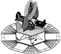
FIG. 4. A sketch of the MAP satellite. The upper half of the spacecraft is cooled by passive radiation to space to get lower noise performance from the optics and the radiometers. Two back-to-back 1.5 m telescopes receive CMBR radiation from spots 141° apart on the sky. Each telescope illuminates 10 horn antennas in its focal plane. The radiometers measure the difference in the powers from pairs of horns on opposite sides of the spacecraft. Twenty radiometer channels capture both polarization modes in each of 5 microwave bands between 20 and 106 GHz. The solar panels (shown deployed) also serve as shields to minimize emission from the sun, Earth, and moon, which are behind the spacecraft at all times. The hexagonal box contains the spacecraft support electronics and the momentum wheels used for attitude control. Data will be sent by telemetry to Earth once a day.

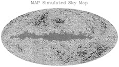
FIG. 5. A computer simulation of the expected MAP results after 2 years of operation. The temperature range is ±100 µK. Note the effect of higher angular resolution compared with Fig. 1. MAP’s wide frequency coverage and high angular resolution will be needed to understand contamination by Galactic radio and dust emission.

is the real map from the COBE/DMR instrument. MAP’s 30 times greater resolution is due to the larger apertures of its back-to-back telescopes (see Fig. 4), and its HEMT amplifier technology developed at the National Radio Astronomy Observatory (35) is 50 times more sensitivity than the mixer-based radiometers used in the COBE/DMR. MAP measures the CMBR anisotropy in 5 frequency bands from 20 to 106 GHz to separate foreground microwave sources from the spectrally unique CMBR anisotropy. Because of its differential design and beam size, MAP’s, angular power spectrum will cover the range 2=l=800. The COBE/DMR measurement will be repeated to establish the large-scale baseline, and at least two of the predicted peaks of the angular power spectrum will be measured, if they exist. PLANCK, scheduled to launch 5 years after MAP, will be able to resolve more peaks and get better data on the expected damping at small angles. Hu and White (36; also see the Hu Web site, http://www.sns.ias.edu/~whu/physics/physics.html) show simulated power spectrum results for both satellites, and several theoretical groups have estimated the accuracy to which successful MAP and PLANCK missions can measure important cosmological parameters (11, 12). However, these should be regarded as a rough indication of the potential of these satellites. Much will depend on whether the underlying cosmological model can be independently established from the CMBR anisotropy data or from other methods. Parameter values will depend strongly on the model used, and accuracy of the parameter estimates will depend on the parameter correlations within that model.

Current active development of close-packed interferometers is directed at measuring small-scale CMBR anisotropy (interferometers are being developed at the Mullard Radio Observatory, the California Institute of Technology, and the University of Chicago). The resolution of these instruments will overlap the angular scales measured by the satellites, and they will extend the angular power spectrum down to a few arcminutes. Small-scale anisotropy measurements will be contaminated by emission from point sources, so interferometers are needed to identify those sources and remove them. Thus, the entire range of angular scales where CMBR anisotropy is expected will be examined with high sensitivity in the next decade.

This work was supported in part by the National Science Foundation and the National Aeronautical and Space Administration.

1. Fixsen, D.J., Cheng, E.S., Gales, J.M., Mather, J.C., Shafer, R.A. & Wright, E.L. (1996) Astrophys. J. 473, 576–587.

2. Bennett, C.L., Banday, A.J., Gorski, K.M., Hinshaw, G., Jackson, P., Keegstra, P., Kogut, A., Smoot, G.F., Wilkinson, D.T. & Wright, E.L. (1996) Astrophys. J. 464, L1–L4.

3. Smoot, G.F., Bennett. C.L., Kogut, A., Wright, E.L., Aymon. J., et al. (1992) Astrophys. J. 396, L1–L5.

4. Kogut, A., Banday, A.J., Bennett, C.L., Gorski, K.M., Hinshaw. G., et al. (1996) Astrophys. J. 470, 653–673.

5. Kogut, A., Smoot, G.F., Bennett, C.L., Wright, E.L., Aymon, J., et al. (1992) Astrophys. J. 401, 1–18.

6. Kogut, A., Banday, A.J., Bennett. C.L., Gorski, K.M., Hinshaw, G., Smoot, G.F. & Wright, E.L. (1996) Astrophys. J. 464, L5–L9.

7. Tegmark, M. & Efstathiou, G. (1995) Mon. Not. R. Astron. Soc. 281, 1297–1314.

8. Peebles, P.J.E. & Yu, J.T. (1970) Astrophys. J. 162, 815–836.

9. Bond, J.R. & Efstathiou, G. (1987) Mon. Not. R. Astron. Soc. 226, 655–687.

10. Hu W., Sugiyama, N. & Silk, J. (1997) Nature (London) 386, 37–43.

11. Jungman, G., Kamionkowski, M., Kosowsky, A. & Spergel, D.N. (1996) Phys. Rev. D 54, 1332–1344.

12. Hu, W. & White, M. (1996) Astrophys. J. 471, 30–51.

13. Bond. R. (1998) Proc. Natl. Acad. Sci. USA 95, 35–41.

14. Ruhl, J., Dragovan, M., Platt, S.R., Kovac, J. & Novak. G. (1995) Astrophys. J. 453, L1–L4.

15. Tucker, G.S., Griffin, G.S., Nguyen, H.T. & Peterson, J.B. (1993) Astrophys. J. 419, L45–L48.

16. Platt, S.R., Kovac, J., Dragovan, M.. Peterson, J.B. & Ruhl. J.E. (1997) Astrophys. J. 475, L1–L4.

17. Piccirillo, L., Femenia, B., Kachwala, N., Rebolo, R., Limon, M., Gutierrez, C.M., Nicholas, J., Schaefer, R.K. & Watson, R.A. (1997) Astrophys. J. 475, L77–L80.

18. Lim, M.A., Clapp. A.C., Devlin, M.J., Figueiredo, N., Gundersen, J.O., Hanany, S., Hristov, V.V., Lange, A.E., Lubin, P.M., Meinhold, P.R., Richards, P.L., Staren, J.W., Smoot. G.F. & Tanaka, S.T. (1996) Astrophys. J. 469, L69–L72.

19. Tanaka, S.T., Clapp, A.C., Devlin, M.J., Figueiredo, N., Gundersen, J.O., Hanany, S., Hristov, V.V., Lange, A.E., Lim, M.A., Lubin, P.M., Meinhold, P.R., Richards, P.L., Smoot, G.F. & Staren, J. (1996) Astrophys. J. 468, L81–L84.

20. de Bernardis, P., Aquilini, E., Boscaleri, A., De Petris, M., D’Andreta, G., Gervasi, M., Kreysa, E., Martinis. L., Masi, S., Palumbo, P. & Scaramuzzi, F. (1994) Astrophys. J. 422, L33–L36.

21. Cheng, E.S., Cottingham, D.A., Fixsen, D.J., Inman, C.A., Kowitt, M.S., Meyer, S.S., Page. L.A., Puchalla, J.L., & Silverberg, R.F. (1994) Astrophys. J. 422, L37–L40.

22. Tucker, G.S., Gush, H.P., Halpern, M. & Shinkoda, I. (1997) Astrophys. J. 475, L73–L76.

23. Netterfield, C.B., Devlin, M.J., Jarosik, N., Page, L. & Wollack, E.J. (1997) Astrophys. J. 474, 47–66.

24. Wollack, E.J., Devlin, M.J., Jarosik. N., Netterfield, C.B., Page, L. & Wilkinson, D. (1997) Astrophys. J. 476, 440–457.

25. Hancock, S., Davies, R.D., Lasenby, A.N., Gutierrez de la Cruz, C.M., Watson, R.A., Rebolo, R. & Beckman, J.E. (1994) Nature (London) 367, 333–338.

26. Fomalont, E.B., Partridge, R.B., Lowenthal, J.D. & Windhorst, R.A. (1993) Astrophys. J. 404, 8–20.

27. Scott, P.F., Saunders, R., Pooley. G., O’Sullivan, C., Lasenby. A.N., Jones, M., Hobson, M.P., Duffett-Smith, P.J. & Baker, J. (1996) Astrophys. J. 461, L1–L4.

28. Page, L.A. (1997) in Proceedings of the Third International School of Particle Astrophysics, Generation of Large Scale Cosmological Structure. Erice. Sicily, Nov. 3–13, 1996. NATO AFI Series, eds. Schramm. D. & Galeotti, P. (Kluwer, Dordrecht), in press.

29. Ratra, B., Sugiyama. N., Banday. A.J. & Gorski, K.M. (1997) Astrophys. J. 481, 22–33.

30. Ganga, K., Cheng, E., Meyer, S. & Page, L. (1993) Astrophys. J. 410, L57–L60.

31. Netterfield, B., Devlin, M.J., Jarosik, N., Page, L. & Wollack. E.J. (1997) Astrophys. J. 474, 47–66.

32. Rees. M. (1968) Astrophys. J. 153, L1–L4.

33. Crittenden, R.G., Coulson, D. & Turok. N. (1995) Phys. Rev. D 52, 5402–5406.

34. Seljak, U. & Zaldarriaga, M. (1997) Phys. Rev. D 55,1830–1840.

35. Pospieszalski, M.W., Lakatosh, W.J., Wollack, E., Nguyan, L.D., Le, M., Lui, M. & Liu, T. (1997) in Proceedings of the 1997 IEEE MTT-S International Microwave Symposium, Denver, CO. June 8–13, 1997, IEEE MTT-S Digest, pp. 1285–1288.

36. Hu, W. & White, M. (1996) Astrophys. J. 471, 30–51.