(NAS Colloquium) Carbon Dioxide and Climate Change (1997)

Proc. Natl. Acad. Sci. USA

Vol. 94, pp. 8314–8320, August 1997

Colloquium Paper

This paper was presented at a colloquium entitled “Carbon Dioxide and Climate Change,” organized by Charles D. Keeling, held November 13–15, 1995, at the National Academy of Sciences, Irvine, CA.

T. M. L. WIGLEY *, P. D. JONES ^†, AND S. C. B. RAPER ^†

*National Center for Atmospheric Research, P.O. Box 3000, Boulder, CO 80307-3000; and ^†Climatic Research Unit, University of East Anglia, Norwich NR4 7TJ, United Kingdom

ABSTRACT Global, near-surface temperature data sets and their derivations are discussed, and differences between the Jones and Intergovernmental Panel on Climate Change data sets are explained. Global-mean temperature changes are then interpreted in terms of anthropogenic forcing influences and natural variability. The inclusion of aerosol forcing improves the fit between modeled and observed changes but does not improve the agreement between the implied climate sensitivity value and the standard model-based range of 1.5–4.5°C equilibrium warming for a CO₂doubling. The implied sensitivity goes from below the model-based range of estimates to substantially above this range. The addition of a solar forcing effect further improves the fit and brings the best-fit sensitivity into the middle of the model-based range. Consistency is further improved when internally generated changes are considered. This consistency, however, hides many uncertainties that surround observed data/model comparisons. These uncertainties make it impossible currently to use observed global-scale temperature changes to narrow the uncertainty range in the climate sensitivity below that estimated directly from climate models.

Observations from land-based meteorological stations and ships at sea have been compiled, corrected for nonmeteorological biases, interpolated to a regular grid, and area-averaged to estimate changes in global-mean temperature over the past century or so. These data show an overall warming trend of about 0.5°C, with marked shorter time scale variability from year to year and decade to decade. It is suspected that part of the long-term warming trend is due to human activities, but determining just how much of the trend is human-induced is a difficult task. This paper describes the data and their development, and interprets the changes that have occurred in terms of anthropogenic and natural causal factors.

The primary data sets are those from land and marine areas. Extensive reviews of these data have been given by the Intergovernmental Panel on Climate Change (IPCC) (1, 2 and 3). Over land, the main data sets are those of Vinnikov et al. (4), Hansen and Lebedeff (5, 6), and Jones et al. (7, 8). The Hansen and Jones data sets are continually updated. Only the Jones data set has undergone rigorous quality control, and it is these data that are used in the standard IPCC global- and hemispheric-mean time series. The different land data sets have been compared in ref. 9. The Jones land data set has recently been updated through the addition of new historical data and a change of reference period from 1951–1970 to 1961–1990 (10). At the hemispheric- and global-mean levels, the effect of this update is small.

The two main marine data sets are those of Jones et al. (ref. 9; see also ref. 11) and the U.K. Meteorological Office (UKMO) (12, 13). These two data sets have overlapping primary source material but differ in the way that they are corrected for instrumentation changes. The Jones et al. marine data set uses UKMO data from 1987 onward and COADS (Comprehensive Ocean-Atmosphere Data Set) data (14) before 1987. The data used in compiling area averages are sea surface temperature data. Marine air temperature data exist, but it is more difficult to correct these for instrumentation problems. Where reliable corrections can be made, the sea surface temperature and marine air temperature data agree almost perfectly (13).

For global-mean (i.e., land plus marine) data, there are two data sets in common usage, the Jones data as listed in Trends ‘93 (15), which combine the older Jones land data (7, 8) with the Jones marine data, and the standard IPCC data set, which combines the newer Jones land data (10) with the UKMO marine data. Refs. 9 and 12 give details on how the land and marine data sets are merged. Because of the history of their development, these global data sets use different reference periods (Jones, 1950–1979; IPCC, 1961–1990).

Numerous corrections have to be made to both the land data and the marine data to remove or correct for nonclimatological influences; extensive discussions have been given in refs. 1, 2, 9, 12, 13, 16, and elsewhere. Small residual biases may remain, but these are judged to cause errors in the overall global-mean trend of, at most, 0.1°C. Trend uncertainties also arise because of incomplete coverage; even now, there are no direct measurements for large areas of the southern oceans, although temperature data for these areas can be derived using satellite data (12, 13). Coverage changes add another element of uncertainty to the trend. IPCC (1, 2) judges the overall trend uncertainty to be ±0.15°C.

Fig. 1 shows the standard IPCC global-mean temperature series compared with the Jones data. Differences arise for five main reasons: (i) because of the different reference periods used (corrected for approximately in Fig. 1); (ii) because of differences in the raw marine data sets (the UKMO data set is somewhat more comprehensive); (iii) because of differences in the method used to correct for marine instrumentation changes (discussed extensively in refs. 9, 12, 13, and 16); (iv) because of different ways in which the global means are calculated; and (v) because of small differences in the land data sets.

The first reason, the effect of different reference periods, gives a difference of 0.046°C or 0.058°C, depending on how the data sets are compared. Over 1950–1979, the Jones data have a global mean of -0.005°C, whereas the IPCC data have a mean of -0.051°C; over 1961–1990, the means are 0.083°C and

0.025°C, respectively. Note that neither data set has a global-mean value of precisely zero over its reference period. Primarily, this is because the reference period applies to the individual grid points and because there are coverage changes over the reference periods. In the Jones data set, the land and marine components have different reference periods. For compatibility in merging the data sets, the land data have to have their reference period adjusted from 1951–1970 to 1950–1979, an adjustment that can only be made approximately. This adjustment is not a problem with the IPCC data because both land and marine components use the same reference period (1961–1990). For land station data to be included in the analysis, however, full reference-period coverage was not required; only a minimum of 20 out of 30 years was needed. This can lead to biases in the anomalies relative to the reference period, which are reflected in the spatial mean anomaly averaged over the reference period. In Fig. 1, both data sets have been adjusted to have zero means over 1961– 1990 by subtraction of 0.025°C from the IPCC data and 0.083°C from the Jones data.

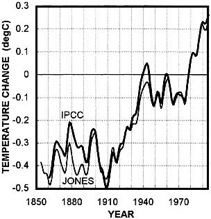
FIG. 1. Comparison of Jones and IPCC global-mean temperature data. Both data sets have been adjusted to have zero means over 1961–1990, and the annual data were then filtered with a 13-point Gaussian filter to highlight decadal and longer time scale changes. Data up to and including 1995 have been used.

The second reason for differences (raw marine data differences) has not been specifically quantified, but it is likely to be relatively small. The third reason (different correction methods) is more important. Below, the combined influences of these two effects are calculated by differencing. To do this, we assume the effect of land data differences (the fifth reason) is negligible, calculate the effect of the fourth reason independently, and subtract this from the difference between the data sets after the effect of the first reason has been removed (see above and Fig. 1).

The fourth reason (different hemispheric averaging methods) has not previously been discussed and is quantified here for the first time (to our knowledge). The two different methods are as follows. In calculating the global mean for the IPCC data set, the data for individual grid boxes are simply area-weighted and averaged. Because the fractional coverage in each hemisphere varies with time, with a relatively greater fraction covered in the Northern Hemisphere in the earlier years, this method may potentially bias the global mean toward the Northern Hemisphere in these years. The Jones global mean is calculated by area-averaging the hemispheres separately first and then averaging the hemispheric means. This method may put undue weight on the sparsely covered Southern Hemisphere in the early years. It is impossible to decide a priori which method is better.

Fig. 2 shows the difference between the IPCC data recalculated using the Jones method and the standard IPCC values (recalculated values minus original values). This isolates the effect of the fourth reason. The differences are small and somewhat erratic, with no overall trend.

Fig. 3 shows the residual difference, Jones data minus recalculated IPCC data, after adjustment of both data sets for the effect of reference-period differences. This plot has been calculated by subtracting the “error” shown in Fig. 2 from the annual data used to produce Fig. 1 This essentially isolates the influences of the different sea surface temperature data sets and the different ways these data sets have been corrected for instrumental biases. The low-frequency changes in this plot arise largely from the different instrumentation correction schemes, whereas the shorter time scale differences mainly reflect differences in the raw data. A clear overall trend (arising mainly over the period 1880–1910) is evident. This trend is reflected in the data differences shown in Fig. 1 and explains why the Jones data have a slightly greater overall warming trend than the IPCC data.

Why has the globe warmed? Because we are confident that human activities have substantially changed the atmospheric composition in terms of greenhouse gases (GHGs; especially carbon dioxide) and aerosols, we are also confident that at least part of the observed warming is human-induced. The leading question is how much? To answer this, we first need to estimate the magnitude of the expected anthropogenic warming. To do this requires a knowledge of the anthropogenic forcing change, and a suitable model to convert this forcing to an estimated climate change.

Fig. 4 shows the current central estimate of forcing changes as used in the latest IPCC calculations of global-mean temperature and sea-level change (ref. 17; further details are given in ref. 18). It is clear that CO₂ is the main single factor, but

FIG. 2. Breakdown of differences between the Jones and IPCC global-mean temperature data over 1861–1994: the effect of different area-averaging methods. The differences shown are annual values of the difference IPCC data averaged according to the Jones method minus original IPCC data.

aerosol influences are a close second in importance. Aerosols operate in two different ways to produce a negative forcing effect that is highly spatially heterogeneous compared with the forcing effect of CO₂ (see refs. 19 and 20). In clear sky conditions, sulfate aerosols (derived mainly from SO₂, which is produced, like CO₂, by fossil-fuel combustion) reflect incoming solar radiation—this process is referred to as direct aerosol forcing (19, 20). In addition, there is an indirect cooling effect through the influence of aerosols, acting as cloud condensation nuclei, on cloud albedo (see refs. 21, 22, 23 and 24 ). Biomass burning also produces aerosols, and these are thought to have a net cooling effect too (ref. 25; this paper gives a much larger effect than more recent estimates). These three components give global-mean forcings with central estimates (to 1990) of −0.3 W/m², −0.8 W/m², and −0.2 W/m², respectively (17, 18, 26), for a total aerosol forcing of −1.3 W/m^2. These estimates are all highly uncertain. The most important uncertainty is that for the indirect effect, whose value is judged to lie somewhere between zero and −1.5 W/m² (26).

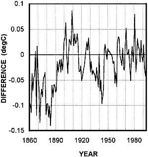
FIG. 3. Breakdown of differences between the Jones and IPCC global-mean temperature data over 1861–1994: combined effect of different marine and land data sets, and different corrections to marine data. Land data set differences have a relatively minor effect. The differences shown are annual values of the difference Jones data minus IPCC data adjusted to use the Jones averaging method, with both data sets adjusted to have the same (zero) 1961–1990 means.

Having determined a past forcing history, this may be used in an upwelling–diffusion energy–balance climate model to estimate the implied global-mean temperature changes. The model used here is that used in refs. 18, 27, and 28, the same model that has been used by IPCC (17). This model has a simplified ocean that accounts for oceanic lag effects, and differentiates the land and ocean areas in each hemisphere to model the spatially disparate forcing effects of sulfate aerosols and to account for the fact that the sensitivity of the climate system to external forcing differs over land and ocean areas. Land and ocean sensitivities are specified externally, allowing uncertainties in these parameters to be explored. The model ocean also has a variable upwelling rate, although this option is not used in the calculations presented here. Further details of the model are given in ref. 18, and its performance compared with coupled ocean/atmosphere general circulation models (O/AGCMs) is described in refs. 17 and 29.

The main factor leading to uncertainties in the global-mean temperature response to any given forcing is the climate sensitivity, usually specified by the equilibrium global-mean warming for a CO₂ doubling (∆T_2×). Any calculations ignoring this uncertainty would be of very limited value. ∆T_2× is thought to lie between 1.5°C and 4.5°C (30), with roughly 90% confidence. The best guess value for ∆T_2× is 2.5°C (30). In the following analyses, the energy balance model has been used with a land/ocean sensitivity differential of 1.3 (explained in ref. 18), and constant upwelling rate, paralleling assumptions made in similar analyses carried out for IPCC (ref. 31, figure 8.4). The results of using the above IPCC forcing data with different global-mean climate sensitivities are given in Fig. 5, Fig. 6, and Fig. 8. For comparison purposes, we use the IPCC observed temperature data set. Because these data have a lower overall warming trend, the implied climate sensitivities are necessarily lower than they would be if we used the Jones data set.

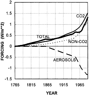
FIG. 4. IPCC estimates of past anthropogenic forcing changes (17). Non-CO₂ GHG forcing is the sum of the effects of CH₄, N₂O, halocarbons, and tropospheric and stratospheric ozone. Aerosol forcing combines direct and indirect sulfate effects and aerosols from biomass burning.

In Fig. 5, only GHG forcing is used (a total of 2.6 W/m² over 1765, the initial model simulation year, to 1990). The modeled and observed results shown have been adjusted to have a common 1861–1900 mean of zero. (The choice of reference period is somewhat arbitrary because only the temperature changes are modeled, not the absolute values.) It is clear from Fig. 5 that the best fit is obtained for a sensitivity below the 1.5°C lower bound of the 90% confidence range. The precise best-fit sensitivity depends on the method used for optimization and the time period over which the results are optimized, and also on the observed data set with which the model’s results are compared. If the root-mean-square error (RMSE) is minimized over the full comparison period, 1861–1994, with no other constraints, and if raw annual IPCC global-mean temperatures are used in the comparison, the best-fit value for ∆T_2× is 1.2°C (see Table 1).

Table 1 gives results for comparisons with two other versions of the IPCC observed data set: IPCC annual data with the influence of the El Niño/Southern Oscillation (ENSO) phenomenon factored out (following ref. 32) and low-pass filtered IPCC data, as shown in Fig. 1. Similar implications arise no matter which data set is used. The ENSO component accounts for roughly 30% of the high-frequency variance and 9% of the total variance in the observed data. With the filtered data, the high-frequency component extracted accounts for 13% of the

total variance. This latter value provides a useful bound on how much of the raw annual data variance can be explained by a deterministic fitting exercise that, like this one, considers only low-frequency forcing (namely ≈87%).

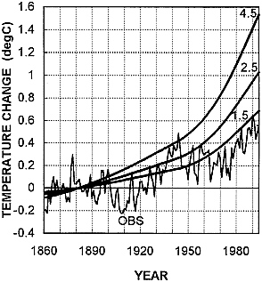
FIG. 5. Observed (OBS; IPCC) and modeled temperature changes for GHG forcing alone. Modeled changes are given for climate sensitivity (∆T_2×) values of 1.5°C, 2.5°C, and 4.5°C. All series have been adjusted to have zero mean over 1861–1900. 1994 is the last year shown. The same results have been presented in the 1995 IPCC report ( 31 ).

The effect of including aerosol forcing is shown in Fig. 6. In this case, the best-fit value of ∆T_2× is clearly higher than the upper 90% value of 4.5°C. If the RMSE against the raw IPCC data is minimized over 1861–1994, the best-fit sensitivity value is 6.3°C (see Table 1). This result is highly sensitive to the assumed amount of aerosol forcing largely because the transient temperature changes (i.e., the model output) become increasingly less sensitive to ∆T_2× as ∆T_2× increases (see ref. 31, and ref. 34, figure 8.1). Table 1 shows that, if the globalmean aerosol forcing is reduced from −1.3 W/m² to −0.9 W/m² (denoted the low case in Table 1), a change that is well within the aerosol forcing uncertainty range, then the best-fit sensitivity drops to 2.6°C.

The addition of aerosol forcing improves the fit compared with the greenhouse-alone case (in terms of RMSE), but only marginally (see Table 1). The higher aerosol forcing case gives a slightly lower RMSE, but this result cannot be used to place more confidence on the higher forcing because RMSE results depend critically on assumptions made regarding other model parameters and the magnitudes of other forcings. Furthermore, as noted above, using the RMSE over the full analysis period is only one of many possible ways to judge a best fit; other methods have different best-fit implications.

Because the climate system varies naturally, one might expect at least part of the low-frequency, century time scale change in global-mean temperature to be due to natural factors. Overall, these factors could have produced a cooling or a warming.

Natural variability can be split into externally forced changes and changes generated purely by internal processes [see also the paper by Keeling and Whorf (43), in this issue of the Proceedings]. The main external causes are solar irradiance changes and the effects of explosive volcanic activity (which produces a cooling aerosol layer in the stratosphere). Because the latter is a short-term effect, lasting at most a few years, and because the main focus of this paper is on the long-term observed trend, volcanic effects will not be considered here, but they can noticeably modify the results of the calculations.

For solar influences, there is strong evidence of significant low-frequency changes in irradiance. These underlie irradiance changes related directly to the solar sunspot cycle (i.e., quasi-cyclic changes with a period of around 11 years) about which there is no dispute. To demonstrate the possible importance of solar forcing, the recent irradiance reconstruction of Hoyt and Schatten (33) is used (see Fig. 7).

The inclusion of solar forcing raises two interesting issues: (i) the importance of the early forcing history (e.g., before 1800) in determining 20th century temperature changes and (ii) the choice of reference level (see ref. 35). Here, we begin our main calculations in 1765 (the initial year for GHG concentration changes) and use the estimated irradiance value in 1765 (1,371.55 W/m²) as the reference level. In other words, we assume that the climate system initially (1765) is in equilibrium with a solar irradiance of 1,371.55 W/m²; by default, therefore, we are assuming also that the irradiance was at this level for all time before 1765 (as illustrated in Fig. 7). An alternative would be to begin at the start of the Hoyt and Schatten solar record (1700) and use the 1700 irradiance value (1,367.52 W/m²) as a reference level. In this case, we are assuming, by default, a constant irradiance level of 1,367.52 W/m² for all times before 1700 (see Fig. 7). In terms of top-of-the-atmosphere forcing, the difference in reference levels amounts to 0.71 W/m² (cf. the IPCC central estimate of 1.3 W/m² for anthropogenic forcing over 1765–1990), with the 1700-start case having a much larger overall (from 1700) forcing trend. It is pertinent to ask what affect does this difference have on temperature changes after 1861 (the start of our observed data analysis period)?

We answer this question by comparing results for the two forcing cases. We note, however, that this comparison probably

overestimates the magnitude of the history and reference-level effects. Using the 1700 value as the reference level may be too extreme because this date is within the anomalously low irradiance period corresponding to the Maunder sunspot minimum—a period often associated with the coldest part of the Little Ice Age. The 1765 value may be too high a reference level because most of the subsequent irradiance values are below this level (see Fig. 7). These two cases, therefore, probably bracket the range of possibilities. When the two simulations are compared, the history/reference-level effect is found to be very small; the difference in warming trend over the period 1861–1994 is only around 0.01°C, with the 1700-start case necessarily having the (very slightly) larger warming trend. This uncertainty is much less than that in the observed data (Fig. 1).

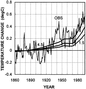
FIG. 6 Observed (OBS; IPCC) and modeled temperature changes for GHG and aerosol forcing. Modeled changes are given for climate sensitivity (∆T_2×) values of 1.5°C, 2.5°C, and 4.5°C. All series have been adjusted to have zero means over 1861–1900. 1994 is the last year shown. The same results have been presented in the 1995 IPCC report (31).

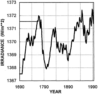
FIG .7. Solar irradiance changes from Hoyt and Schatten (33). Their data span 1700–1992; estimated values are shown to 1994. To obtain top-of-the-atmosphere forcing values (to give changes that are then directly comparable with the anthropogenic forcings shown in Fig. 4), the values shown should be multiplied by 0.175. The main climate model calculations begin in 1765 and assume constant irradiance at the 1765 level before this date, as shown. Similar calculations using 1700 as a starting date with constant irradiance at the 1700 level for the time before 1700 lead to only negligible differences after the mid-19th century.

This is an important result because it demonstrates that the warming since the mid- to late 19th century cannot be considered as a “recovery” from the cold period known as the Little Ice Age, a possibility alluded to in the 1990 IPCC report (1) and sometimes used by greenhouse skeptics as an alternative to anthropogenic forcing as an explanation of the 20th century warming trend. The 1700-start case includes an initial Little Ice Age period (indeed, it assumes that the globe was in a permanent Little Ice Age state before 1700!), yet results for this case differ only negligibly from the 1765-start case in terms of 20th century temperature changes; the memory of the climate system is simply not long enough to “remember” the low forcing interval before 1765.

Full model results for the combined solar-plus-anthropogenic (greenhouse-plus-aerosol) forcing case are shown in Fig. 8. The addition of solar forcing gives a slight improvement in the best fit. The minimum RMSE based on the raw IPCC data drops to 0.117°C from 0.121°C (see Table 1), and the rapid observed warming over 1910–1940 and the subsequent leveling off of the temperature rise are matched more closely than for the pure anthropogenic forcing case. Similar RMSE improvements occur with the other observed data sets (Table 1). In addition, because the overall solar forcing trend is positive, the best-fit climate sensitivity is reduced, from 6.3°C to 3.0°C, based on the raw IPCC data. Using the low aerosol forcing gives an even lower sensitivity, 1.8°C (see Table 1).

Part of the overall trend may also be due to internally generated natural variability; indeed, a considerable fraction of the annual to decadal time scale variability must be due to this factor. As noted above, roughly 13% of the total variance over 1861–1994 is at high frequencies (time scales on the order

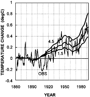
FIG. 8. Observed (OBS; IPCC) and modeled temperature changes for GHG, aerosol, and solar forcing (i.e., as for Fig. 6 but with the solar forcing from Fig. 7 added). Modeled changes are given for climate sensitivity (∆T_2×) values of 1.5°C, 2.5°C, and 4.5°C. All series have been adjusted to have zero means over 1861–1900. 1994 is the last year shown. The same results have been presented in the 1995 IPCC report (31).

of 10 years or less), of which about 30% can be explained by ENSO. On longer time scales, the crucial issue here is whether or not part of the century time scale trend can be attributed to internally generated variability. The magnitude of this possible trend component has been estimated using the simple up-welling–diffusion energy–balance model employed here (see ref. 36) and using more complex coupled O/AGCMs (37). An illustration of this unforced variability is given in Fig. 9, from the GFDL (Geophysical Fluid Dynamics Laboratory) O/AGCM (37). If the O/AGCM data are searched for 134-year trends (i.e., the length of the observational record used here) the maximum global-mean trend is around 0.15°C. Somewhat larger century time scale, internally generated trend values have been given in ref. 36. Both models indicate, however, that only a relatively small (but nonetheless potentially important) fraction of the overall observed trend could be explained by internal processes.

On shorter time scales, natural internally generated trends become more important relative to the anthropogenic signal, a fact that makes interpretation of shorter time scale changes increasingly difficult as the time scale decreases. For example, it has been noted that the observed warming trend over 1910–1940 is considerably larger than that expected from anthropogenic forcing (see Fig. 5 and Fig. 6). It is large, also, compared with the modeled effect of anthropogenic-plus-solar forcing (see Fig. 8). The discrepancy, 0.2–0.3°C over the 30-year period, is, however, within what might be expected due to internally generated variability, which frequently shows trends of similar magnitude in model experiments. Note that the observed trend over this period is uncertain by at least 0.1°C (see Fig. 1).

As an additional consistency check, we note that the residual variability obtained from the best-fit greenhouse/aerosol/solar forcing simulation (RMSE = 0.12°C if the raw IPCC data are used and 0.11°C if ENSO effects are removed) is similar to the average standard deviation over 134-year intervals in the GFDL internal variability simulation (namely, 0.09°C). Because the GFDL variability is a measure of the component that the present deterministic fitting exercise can never account for, this means that we are able to explain almost all of the variance that one could ever hope to explain. Given that the GFDL model underestimates the magnitude of interannual variability related to the ENSO phenomenon, and that the inclusion of volcanic forcing effects should reduce the best-fit RMSE value still further, this is an encouraging result. We note, however, that this result throws little light on which forcing assumption is best because all of the forcings considered here, when the model/observed data fit is optimized, yield similar RMSE values.

FIG. 9. Internally generated variability of global-mean temperature from the GFDL coupled O/AGCM control run. Only the first 200 years of the 1000-year run are shown. A long-term drift component of 0.023°C per century, probably a model artifact, has been removed.

Although there is a quite striking overall consistency in the variance breakdown between the various anthropogenic and natural factors, this consistency does not preclude the possibility of a noticeable and practically significant century time scale trend in the observations due to internal factors. Such a trend could be either positive or negative. Accounting for this possibility introduces an additional element of uncertainty into any attempt to deduce the climate sensitivity from the observational data (38) even when the whole data record is considered. Table 1 shows that, because of external forcing uncertainties that lie well within the range of possibilities, the sensitivity could lie anywhere between 1.7°C and 6.4°C. If, however, part of the trend were internally generated, the range of possibilities may be substantially increased. For example, if 0.1°C of the overall observed warming trend of 0.5°C were internally generated (or, for that matter, the result of errors in the observational data), then the externally forced trend would only be 0.4°C. For any given forcing, the sensitivity required to explain a 0.4°C trend is much less than that required to explain a 0.5°C trend. This uncertainty factor, of course, may operate in either direction.

In attempts to explain the observed warming trend over the past century or so, inclusion of aerosol forcing improves the fit between observed and modeled data (in terms of the minimum RMSE value). However, the agreement between the observationally based (best-fit) sensitivity and the independent model-based range is not improved; the best-fit sensitivity changes from being too low (less than 1.5°C) if GHG forcing alone is used to too high (above 4.5°C) if the IPCC central estimate of aerosol forcing is included. These apparently anomalous sensitivities, however, can be easily reconciled with the model-based range, either through a small reduction in aerosol forcing or by including a solar forcing component. Neither addition changes the RMSE value significantly; including solar forcing leads to a slight improvement.

Alternatively, as noted in ref. 38, a small, internally generated trend could help in reconciling these climate sensitivity differences, especially when considered in conjunction with the external forcing uncertainties. The potential importance of century time scale internal variability as a component of the observed warming has rarely been considered. Any such overall trend could be positive or negative. There is no way to determine whether such a trend component exists, let alone estimate its magnitude, but it is unlikely that it would be zero.

In spite of the likelihood of an (unknowable) internally generated trend component, the model/observed data comparison presented here demonstrates that the observed century time scale global-mean temperature changes are consistent with a dominant anthropogenic influence and secondary influence from solar irradiance increases. The secondary nature of the solar role obtains because the overall solar forcing trend is substantially less than the central anthropogenic forcing estimate of 1.3 W/m². The consistency of this explanation is reinforced by the magnitude of the residuals about the best fit, which is very similar to the magnitude of internally generated natural variability estimated independently from the GFDL coupled O/AGCM.

This consistency, however, does not prove that there has been a large anthropogenic influence. Given uncertainties in the forcing (both anthropogenic and natural), it is still possible that part of the trend has been internally generated. Because

of these various uncertainties, estimates of the value of the climate sensitivity cannot be improved by using observational data alone; the range of possible values for ∆T_2× deduced in this way is substantially larger than the standard model-based range for ∆T_2×, 1.5–4.5°C. It is, however, much more difficult to derive sensitivities below 1.5°C from the observational data than it is to obtain values above 4.5°C.

Where do we go from here? In the most recent IPCC report (31) and in an earlier report (34), it was noted that studies of global-mean temperature alone are insufficient to show a compelling cause–effect relationship between anthropogenic forcing and climate change. Such studies, as shown above, can demonstrate that the observed warming is consistent with a substantial anthropogenic effect on climate but cannot accurately quantify this effect. To show a cause–effect linkage, more sophisticated techniques are required that make use of the patterns of observed climate change, either in the near-surface horizontal (latitude/longitude) plane (39, 40) or in the vertical (zonal mean/height) plane ( 41 , 42 ). Such pattern-based studies have shown increasing and statistically significant similarities between model predictions and observed temperature changes. These results, combined with the evidence from global-mean analyses, provide convincing evidence for a discernible human influence on global climate; but further work is required to better quantify the magnitude of the human influence and reduce uncertainties in the climate sensitivity.

This work was supported by the U.S. Department of Energy (Grant DE-FG02-86ER60397) and the National Oceanic and Atmospheric Administration (Grant NA96AANAG0347). The National Center for Atmospheric Research is sponsored by the National Science Foundation. IPCC temperature data were provided by David Parker, U.K. Meteorological Office.

1. Folland, C. K. , Karl, T. R. & Vinnikov, K. Y. ( 1990 ) in Climate Change: The IPCC Scientific Assessment , eds. Houghton, J. T. , Jenkins, G. J. & Ephraums, J. J. ( Cambridge Univ. Press , Cambridge, U.K. ), pp. 195–238 .

2. Folland, C.K. , Karl, T. R. , Nicholls, N. , Nyenzi, B. S. , Parker, D. E. & Vinnikov, K. Y. ( 1992 ) in Climate Change 1992: The Supplementary Report to the IPCC Scientific Assessment , eds. Houghton, J. T. , Callander, B. A. & Varney, S. K. ( Cambridge Univ. Press , Cambridge, U.K. ), pp. 135–170 .

3. Nicholls, N. , Gruza, G. V. , Jouzel, J. , Karl, T. R. , Ogallo, L. A. & Parker, D. E. ( 1996 ) in Climate Change 1995: The Science of Climate Change , eds. Houghton, J. T. , Meira Filho, L. G. , Callander, B. A. , Harris, N. , Kattenberg, A. & Maskell, K. ( Cambridge Univ. Press , Cambridge, U.K. ), pp. 133–192 .

4. Vinnikov, K. Y. , Groisman, P. Y. & Lugina, K. M. ( 1990 ) J. Clim. 3 , 662–677 .

5. Hansen, J. & Lebedeff, S. ( 1987 ) J. Geophys. Res. 92 , 13345–13372 .

6. Hansen, J. & Lebedeff, S. ( 1988 ) Geophys. Res. Lett. 15 , 323–326 .

7. Jones, P. D. , Raper, S. C. B. , Bradley, R. S. , Diaz, H. F. , Kelly, P. M. & Wigley, T. M. L. ( 1986 ) J. Clim. Appl. Meteorol. 25 , 161–179 .

8. Jones, P. D. , Raper, S. C. B. & Wigley, T. M. L. ( 1986 ) J. Clim. Appl. Meteorol. 25 , 1213–1230 .

9. Jones, P. D. , Wigley, T. M. L. & Farmer, G. ( 1991 ) in Green-house-Gas-Induced Climatic Change: A Critical Appraisal of Simulations and Observations , ed. Schlesinger, M. E. ( Elsevier Science Publishers , Amsterdam ), pp. 153–172 .

10. Jones, P. D. ( 1994 ) J. Clim. 7 , 1794–1802 .

11. Jones, P. D. & Briffa, K. R. ( 1992 ) Holocene 2 , 174–188 .

12. Parker, D. E. , Jones, P. D. , Folland, C. K. & Bevan, A. ( 1994 ) J. Geophys. Res. 99 , 14373–14399 .

13. Parker, D. E. , Folland, C. K. & Jackson, M. ( 1995 ) Clim. Change 31 , 559–600 .

14. Woodruff, S. D. , Slutz, R. J. , Jenne, R. J. & Steurer, P. M. ( 1987 ) Bull. Am. Meteorol. Soc. 68 , 1239–1250 .

15. Jones, P. D. , Wigley, T. M. L. & Briffa, K. R. ( 1994 ) in Trends ‘93: A Compendium of Data on Global Change , eds. Boden, T.A. , Kaiser, D. P. , Sepanski, R. J. & Stoss, F. W. ( Carbon Dioxide Information Analysis Center , Oak Ridge, TN ), pp. 603–608 .

16. Folland, C. K. & Parker, D. E. ( 1995 ) Q. J. R. Meteorol. Soc. 121 , 319–368 .

17. Kattenberg, A. , Giorgi, F. , Grassl, H. , Meehl, G. A. , Mitchell, J. F. B. , Stouffer, R. J. , Tokioka, T. , Weaver, A. J. & Wigley, T. M. L. ( 1996 ) in Climate Change 1995: The Science of Climate Change , eds. Houghton, J. T. , Meira Filho, L. G. , Callander, B. A. , Harris, N. , Kattenberg, A. & Maskell, K. ( Cambridge Univ. Press , Cambridge, U.K. ), pp. 285–357 .

18. Raper, S. C. B. , Wigley, T. M. L. & Warrick, R. A. ( 1996 ) in Sea-Level Rise and Coastal Subsidence: Causes, Consequences and Strategies , eds. Milliman, J. D. & Haq, B. U. ( Kluwer, Dordrecht , The Netherlands ), pp. 11–45 .

19. Charlson, R. J. , Langner, J. , Rodhe, H. , Leovy, C. B. & Warren, S. G. ( 1991 ) Tellus 43AB , 152–163 .

20. Taylor, K. E. & Penner, J. E. ( 1994 ) Nature (London) 369 , 734–737 .

21. Twomey, S. A. , Piepgrass, M. & Wolfe, T. L. ( 1984 ) Tellus 36B , 356–366 .

22. Charlson, R. J. , Lovelock, J. E. , Andreae, M. O. & Warren, S. G. ( 1987 ) Nature (London) 326 , 655–661 .

23. Wigley, T. M. L. ( 1991 ) Nature (London) 349 , 503–506 .

24. Jones, A. , Roberts, D. L. & Slingo, A. ( 1994 ) Nature (London) 370 , 450–463 .

25. Penner, J. E. , Dickinson, R. E. & O’Neill, C. A. ( 1992 ) Science 256 , 1432–1434 .

26. Schimel, D. S. , Alves, D. , Enting, I. , Heimann, M. , Joos, F. , et al. ( 1996 ) in Climate Change 1995: The Science of Climate Change , eds. Houghton, J. T. , Meira Filho, L. G. , Callander, B. A. , Harris, N. , Kattenberg, A. & Maskell, K. ( Cambridge Univ. Press , Cambridge, U.K. ), pp. 65–131 .

27. Wigley, T. M. L. & Raper, S. C. B. ( 1987 ) Nature (London) 330 , 127–131 .

28. Wigley, T. M. L. & Raper, S. C. B. ( 1992 ) Nature (London) 357 , 293–300 .

29. Raper, S. C. B. & Cubasch, U. ( 1996 ) Geophys. Res. Lett. 23 , 1107–1110 .

30. Mitchell, J. F. B. , Manabe, S. , Meleshko, V. & Tokioka, T. ( 1990 ) in Climate Change: The IPCC Scientific Assessment , eds. Houghton, J. T. , Jenkins, G. J. & Ephraums, J. J. ( Cambridge Univ. Press , Cambridge, U.K. ), pp. 131–172 .

31. Santer, B. D. , Wigley, T. M. L. , Barnett, T. P. & Anyamba, E. ( 1996 ) in Climate Change 1995: The Science of Climate Change , eds. Houghton, J. T. , Meira Filho, L. G. , Callander, B. A. , Harris, N. , Kattenberg, A. & Maskell, K. ( Cambridge Univ. Press , Cambridge, U.K. ), pp. 407–443 .

32. Jones, P. D. ( 1988 ) Clim. Monit. 17 , 80–9 .

33. Hoyt, D. V. & Schatten, K. H. ( 1993 ) J. Geophys. Res. 98 , 18895–18906 .

34. Wigley, T. M. L. & Barnett, T. P. ( 1990 ) in Climate Change: The IPCC Scientific Assessment , eds. Houghton, J. T. , Jenkins, G. J. & Ephraums, J. J. ( Cambridge Univ. Press , Cambridge, U.K. ), pp. 239–255 .

35. Wigley, T. M. L. & Raper, S. C. B. ( 1990 ) Geophys. Res. Lett. 17 , 2169–2172 .

36. Wigley, T. M. L. & Raper, S. C. B. ( 1990 ) Nature (London) 344 , 324–327 .

37. Stouffer, R.J. , Manabe, S. & Vinnikov, K.Y. ( 1994 ) Nature (London) 367 , 634–636 .

38. Wigley, T. M. L. & Raper, S. C. B. ( 1991 ) in Climate Change: Science, Impacts and Policy , eds. Jäger, J. & Ferguson, H. L. ( Cambridge Univ. Press , Cambridge, U.K. ), pp. 231–242 .

39. Santer, B. D. , Taylor, K. E. , Wigley, T. M. L. , Penner, J. E. , Jones, P. D. & Cubasch, U. ( 1995 ) Clim. Dyn. 12 , 77–100 .

40. Mitchell, J. F. B. , Johns, T. C. , Gregory, J. M. & Tett, S. F. B. ( 1995 ) Nature (London) 376 , 501–504 .

41. Santer, B. D. , Taylor, K. E. , Wigley, T. M. L. , Johns, T. C. , Jones, P. D. , Karoly, D. J. , Mitchell, J. F. B. , Oort, A. H. , Penner, J. E. , Ramaswamy, V. , Schwarzkopf, M. D. , Stouffer, R. J. & Tett, S. F. B. ( 1996 ) Nature (London) 382 , 39–46 .

42. Tett, S. F. B. , Mitchell, J. F. B. , Parker, D. E. & Allen, M. R. ( 1996 ) Science 274 , 1170–1173 .

43. Keeling, C. D. & Whorf, T. P. ( 1997 ) Proc. Natl. Acad. Sci. USA 94 , 8321–8328 .