
Chapter 4
Invited Session on Record Linkage Methodology
Chair: Nancy Kirkendall, Office of Management and Budget
Authors:
Thomas R.Belin, University of California—Los Angeles, and Donald B.Rubin, Harvard University
Michael D.Larsen, Harvard University
Fritz Scheuren, Ernst and Young, LLP and William E.Winkler, Bureau of the Census
A Method for Calibrating False-Match Rates in Record Linkage*
Thomas R.Belin, UCLA and Donald B.Rubin, Harvard University
Specifying a record-linkage procedure requires both (1) a method for measuring closeness of agreement between records, typically a scalar weight, and (2) a rule for deciding when to classify records as matches or non matches based on the weights. Here we outline a general strategy for the second problem, that is, for accurately estimating false-match rates for each possible cutoff weight. The strategy uses a model where the distribution of observed weights are viewed as a mixture of weights for true matches and weights for false matches. An EM algorithm for fitting mixtures of transformed-normal distributions is used to find posterior modes; associated posterior variability is due to uncertainty about specific normalizing transformations as well as uncertainty in the parameters of the mixture model, the latter being calculated using the SEM algorithm. This mixture-model calibration method is shown to perform well in an applied setting with census data. Further, a simulation experiment reveals that, across a wide variety of settings not satisfying the model's assumptions, the procedure is slightly conservative on average in the sense of overstating false-match rates, and the one-sided confidence coverage (i.e., the proportion of times that these interval estimates cover or overstate the actual false-match rate) is very close to the nominal rate.
KEY WORDS: Box-Cox transformation; Candidate matched pairs; EM algorithm; Mixture model; SEM algorithm; Weights.
1. AN OVERVIEW OF RECORD LINKAGE AND THE PROBLEM OF CALIBRATING FALSE-MATCH RATES
1.1 General Description of Record Linkage
Record linkage (or computer matching, or exact matching) refers to the use of an algorithmic technique to identify records from different data bases that correspond to the same individual. Record-linkage techniques are used in a variety of settings; the current work was formulated and first applied in the context of record linkage between the census and a large-scale postenumeration survey (the PES), which comprises the first step of an extensive matching operation conducted to evaluate census coverage for subgroups of the population (Hogan 1992). The goal of this first step is to declare as many records as possible “matched” without an excessive rate of error, thereby avoiding the cost of the resulting manual processing for all records not declared “matched.”
Specifying a record-linkage procedure requires both a method for measuring closeness of agreement between records and a rule using this measure for deciding when to classify records as matches. Much attention has been paid in the record-linkage literature to the problem of assigning “weights” to individual fields of information in a multivariate record and obtaining a “composite weight” that summarizes the closeness of agreement between two records (see, for example, Copas and Hilton 1990; Fellegi and Sunter 1969; Newcombe 1988; and Newcombe, Kennedy, Axford, and James 1959). Somewhat less attention has been paid to the problem of deciding when to classify records as matches, although various approaches have been offered by Tepping (1968), Fellegi and Sunter (1969), Rogot, Sorlie, and Johnson (1986), and Newcombe (1988). Our work focuses on the second problem by providing a predicted probability of match for two records, with associated standard error, as a function of the composite weight.
The context of our problem, computer matching of census records, is typical of record linkage. After data collection, preprocessing of data, and determination of weights, the next step is the assignment of candidate matched pairs where each pair of records consists of the best potential match for each other from the respective data bases (cf. “hits” in Rogot, Sorlie, and Johnson 1986; “pairs” in Winkler 1989; “assigned pairs” in Jaro 1989). According to specified rules, a scalar weight is assigned to each candidate pair, thereby ordering the pairs. The final step of the record linkage procedure is viewed as a decision problem where three actions are possible for each candidate matched pain declare the two records matched, declare the records not matched, or send both records to be reviewed more closely (see, for example, Fellegi and Sunter 1969). In the motivating problem at the U.S. Census Bureau, a binary choice is made between the alternatives “declare matched” versus “send to followup,” although the matching procedure attempts to draw distinctions within the latter group to make manual matching easier for follow-up clerks. In such a setting, a cutoff weight is needed above which records are declared matched; the false-match rate is then defined as the number of falsely matched pairs divided by the number of declared matched pairs. Particularly relevant for any such decision problem is an accurate method for assessing the probability that a candidate matched pair is a correct match as a function of its weight.
1.2 The Need for Better Methods of Classifying Records as Matches or Nonmatches
Belin (1989a, 1989b, 1990) studied various weighting procedures (including some suggested by theory, some used in practice, and some new simple ad hoc weighting schemes) in the census matching problem and reached three primary
|
* |
Thomas R.Belin is Assistant Professor. Department of Biostatistics. UCLA School of Public Health. Los Angeles. CA, 90024. Donald B.Rubin is Professor. Department of Statistics. Harvard University. Cambridge, MA, 02138. The authors would like to thank William Winkler of the U.S. Census Bureau for a variety of helpful discussions. The authors also gratefully acknowledge the support of Joint Statistical Agreements 89–07, 90–23, and 91– 08 between the Census Bureau and Harvard University, which helped make this research possible. Much of this work was done while the first author was working for the Record Linkage Staff of the Census Bureau: the views expressed are those of the authors and do not necessarily reflect those of the Census Bureau. |
conclusions. First, different weighting procedures lead to comparable accuracy in computer matching. Second, as expected logically and from previous work (e.g., Newcombe 1988, p. 144), the false-match rate is very sensitive to the setting of a cutoff weight above which records will be declared matched. Third, and more surprising, current methods for estimating the false-match rate are extremely inaccurate, typically grossly optimistic.
To illustrate this third conclusion, Table 1 displays empirical findings from Belin (1990) with test-census data on the performance of the procedure of Fellegi and Sunter (1969), which relies on an assumption of independence of agreement across fields of information. That the Fellegi-Sunter procedure for estimating false-match rates does not work well (i. e., is poorly calibrated) may not be so surprising in this setting, because the census data being matched do not conform well to the model of mutual independence of agreement across the fields of information (see, for example, Kelley 1986 and Thibaudeau 1989). Other approaches to estimating false-match rates that rely on strong independence assumptions (e.g., Newcombe 1988) can be criticized on similar grounds.
Although the Fellegi-Sunter approach to setting cutoff weights was originally included in census/PES matching operations (Jaro 1989), in the recent past (including in the 1990 Census) the operational procedure for classifying record pairs as matches has been to have a human observer establish cutoff weights manually by “eyeballing ” lists of pain of records brought together as candidate matches. This manual approach is easily criticized, both because the error properties of the procedure are unknown and variable and because, when linkage is done in batches at different times or by different persons, inconsistent standards are apt to be applied across batches.
Another idea is to use external data to help solve this classification problem. For example, Rogot, Sorlie, and Johnson (1986) relied on extreme order statistics from pilot data to determine cutoffs between matches and nonmatches; but this technique can be criticized, because extreme order statistics may vary considerably from sample to sample, especially when sample sizes are not large. One other possibility, discussed by Tepping (1968), requires clerical review of samples from the output of a record-linkage procedure to provide
Table 1. Performance of Fellegi-Sunter Cutoff Procedure on 1986 Los Angeles Test-Census Data
|
Acceptable false-match rate specified by the user of matching program |
Observed false-match rate among declared matched pairs |
|
.05 |
.0627 |
|
.04 |
.0620 |
|
.03 |
.0620 |
|
.02 |
.0619 |
|
.01 |
.0497 |
|
10−3 |
.0365 |
|
10−4 |
.0224 |
|
10−5 |
.0067 |
|
10−6 |
.0067 |
|
10−7 |
.0067 |
feedback on error rates to refine the calibration procedure. Such feedback is obviously desirable, but in many applications, including the census/PES setting, it is impossible to provide it promptly enough.
A more generally feasible strategy is to use the results of earlier record-linkage studies in which all candidate matched pairs have been carefully reviewed by clerks. This type of review is common practice in operations conducted by the Census Bureau. Each such training study provides a data set in which each candidate pair has its weight and an outcome, defined as true match or false match, and thus provides information for building a model to give probability of match as a function of weight.
1.3 A Proposed Solution to the Problem of Calibrating Error Rates
There are two distinct approaches to estimating the relationship between a dichotomous outcome, Zi = 1 if match and Zi = 0 if nonmatch, from a continuous predictor, the weight, Wi: the direct approach, typified by logistic regression, and the indirect approach, typified by discriminant analysis. In the direct approach, an iid model is of the form f(Zi|Wi, ν) × g(Wi|ζ), where g(Wi|ζ), the marginal distribution of Wi, is left unspecified with ζ a priori independent of ν. In the indirect approach, the iid model is of the form h(Wi|Zi,φ)[λZi(1 − λ)(1−Zi)], where the first factor specifies, for example, a normal conditional distribution of Wi for Zi = 0 and for Zi = 1 with common variance but different means, and the second factor specifies the marginal probability of Zi = 1, λ, which is a priori independent of φ. Under this approach, P(Zi|Wi) is found using Bayes's theorem from the other model specifications as a function of φ and λ. Many authors have discussed distinctions between the two approaches, including Halperin, Blackwelder, and Verter (1971), Mantel and Brown (1974), Efron (1975), and Dawid (1976).
In our setting, application of the direct approach would involve estimating f(Zi|Wi, ν) in observed sites where determinations of clerks had established Zi, and then applying the estimated value of ν to the current site with only Wi observed to estimate the probability of match for each candidate pair. If the previous sites differed only randomly from the current sites, or if the previous sites were a subsample of the current data selected on Wi, then this approach would be ideal Also, if there were many previous sites and each could be described by relevant covariates, such as urban/ rural and region of the country, then the direct approach could estimate the distribution of Z as a function of W and covariates and could use this for the current site. Limited experience of ours and of our colleagues at the Census Bureau, who investigated this possibility using 1990 Census data, has resulted in logistic regression being rejected as a method for estimating false-match rates in the census setting (W.E.Winkler 1993, personal communication).
But the indirect approach has distinct advantages when, as in our setting, there can be substantial differences among sites that are not easily modeled as a function of covariates and we have substantial information on the distribution of weights given true and false matches, h(• | •). In particular,
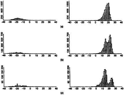
Figure 1. Histograms of Weights for True and False Matches by Site: (a) St. Louis; (b) Columbia; (c) Washington.
with the indirect approach, the observed marginal distribution of Wi in the current site is used to help estimate P(Zi|Wi) in this site, thereby allowing systematic site to site differences in P(Zi|Wi). In addition, there can be substantial gains in efficiency using the indirect approach when normality holds (Efron 1975), especially when h(Wi|Zi = 1, φ) and h(Wi|Zi = 0, φ) are well separated; (that is, when the number of standard deviations difference between their means is large).
Taking this idea one step further, suppose that previous validated data sets had shown that after a known transformation, the true-match weights were normally distributed, and that after a different known transformation, the false-match weights were normally distributed. Then, after inverting the transformations, P(Zi|Wi) could be estimated in the current site by fitting a normal mixture model, which would estimate the means and variances of the two normal components (i.e., φ) and the relative frequency of the two components (i.e., λ), and then applying Bayes's theorem. In this example, instead of assuming a common P(Zi|Wi) across all sites, only the normality after the fixed transformations would be assumed common across sites. If there were many sites with covariate descriptors, then (λ, φ) could be modeled as a function of these, for example, a linear model structure on the normal means.
To illustrate the application of our work, we use available test-census data consisting of records from three separate sites of the 1988 dress rehearsal Census and PES: St. Louis, Missouri, with 12,993 PES records; a region in East Central Missouri including Columbia, Missouri, with 7,855 PES records; and a rural area in eastern Washington state, with only 2,318 records. In each site records were reviewed by clerks, who made a final determination as to the actual match status of each record; for the purpose of our discussion, the clerks ' determinations about the match status of record pairs are regarded as correct The matching procedures used in the 1988 test Census have been documented by Brown et al. (1988), Jaro (1989), and Winkler (1989). Beyond differences in the sizes of the PES files, the types of street addresses in the areas offer considerably different amounts of information for matching purposes; for instance, rural route addresses, which were common in the Washington site but almost nonexistent in the St. Louis site, offer less information for matching than do most addresses commonly found in urban areas.
Figure 1 shows histograms of both true-match weights and false-match weights from each of the three sites. The bimodality in the true-match distribution for the Washington site appears to be due to some record pairs agreeing on address information and some not agreeing. This might generate concern, not so much for lack of fit in the center of the distribution as for lack of fit in the tails, which are essential to false-match rate estimation. Of course, it is not surprising that validated data dispel the assumption of normality for true-match weights and false-match weights. They do, however—at least at a coarse level in their apparent skewness— tend to support the idea of a similar nonnormal distributional shape for true-match weights across sites as well as a similar nonnormal distributional shape for false-match weights across sites. Moreover, although the locations of these distributions change from she to site, as do the relative frequencies of the true-match to the false-match components, the relative spread of the true to false components is similar across sites.
These observations lead us to formulate a transformed-normal mixture model for calibrating false-match rates in record-linkage settings. In this model, two power (or Box-Cox) transformations are used to normalize the false-match weights and the true-match weights, so that the observed raw weights in a current setting are viewed as a mixture of two transformed normal observations.
Mixture models have been used in a wide variety of statistical applications (see Titterington, Smith, and Makov 1985, pp. 16–21, for an extensive bibliography). Power transformations are also used widely in statistics, prominently in an effort to satisfy normal theory assumptions in regression settings (see, for example, Weisberg 1980, pp. 147–151). To our knowledge, neither of these techniques has been utilized in record linkage operations, nor have mixtures of transformed-normal distributions, with different transformations in the groups, appeared previously in the statistical literature, even though this extension is relatively straightforward. The most closely related effort to our own of which we are aware is that of Maclean, Morton, Elston, and Yee (1976), who used a common power transformation for different components of a mixture model, although their work focused on testing for the number of mixture components.
Section 2 describes the technology for fitting mixture models with components that are normally distributed after application of a power transformation, which provides the statistical basis for the proposed calibration method. This section also outlines the calibration procedure itself, including the calculation of standard errors for the predicted false-match rate. Section 3 demonstrates the performance of the method in the applied setting of matching the Census and PES, revealing it to be quite accurate. Section 4 summarizes a simulation experiment to gauge the performance of the calibration procedure in a range of hypothetical settings and this too supports the practical utility of the proposed calibration approach. Section 5 concludes the article with a brief discussion.
2. CALIBRATING FALSE-MATCH RATES IN RECORD LINKAGE USING TRANSFORMED-NORMAL MIXTURE MODELS
2.1 Strategy Based on Viewing Distribution of Weights as Mixture
We assume that a univariate composite weight has been calculated for each candidate pair in the record-linkage problem at hand, so that the distribution of observed weights is a mixture of the distribution of weights for true matches and the distribution of weights for false matches. We also assume the availability of at least one training sample in which match status (i.e., whether a pair of records is a true match or a false match) is known for all record pairs. In our applications, training samples come from other geographical locations previously studied. We implement and study the following strategy for calibrating the false-match rate in a current computer-matching problem:
-
Use the training sample to estimate “global” parameters, that is, the parameters of the transformations that normalize the true- and false-match weight distributions and the parameter that gives the ratio of variances between the two components on the transformed scale. The term “global” is used to indicate that these parameters are estimated by data from other sites and are assumed to be relatively constant from site to site, as opposed to “site-specific ” parameters, which are assumed to vary from site to site and are estimated only by data from the current site.
-
Fix the values of the global parameters at the values estimated from the training sample and fit a mixture of transformed-normal distributions to the current site's weight data to obtain maximum likelihood estimates (MLE's) and associated standard errors of the component means, component variances, and mixing proportion. We use the EM algorithm (Dempster, Laird, and Rubin 1977) to obtain MLE 's and the SEM algorithm (Meng and Rubin 1991) to obtain asymptotic standard errors.
-
For each possible cutoff level for weights, obtain a point estimate for the false-match rate based on the parameter estimates from the model and obtain an estimate of the standard error of the false-match rate. In calculating standard errors, we rely on a large-sample approximation that makes use of the estimated covariance matrix obtained from the SEM algorithm.
An appealing modification of this approach, which we later refer to as our “full strategy,” reflects uncertainty in global parameters through giving them prior distributions. Then, rather than fixing the global parameters at their estimates from the training sample, we can effectively integrate over the uncertainty in the global parameters by modifying Step 2 to be:
2'. Draw values of the global parameters from their posterior distribution given training data, fix global parameters at their drawn values, and fit a mixture of transformed-normal distributions to the current weight data to obtain MLE's (and standard errors) of site-specific parameters;
and adding:
4. Repeat Steps 2' and 3 a few or several times, obtaining false-match rate estimates and standard errors from each repetition, and combine the separate estimates and standard errors into a single point estimate and standard error that reflect uncertainty in the global parameters using the multiple imputation framework of Rubin (1987).
We now describe how to implement each of these steps.
2.2 Using a Training Sample to Estimate Global Parameters
Box and Cox (1964) offered two different parameterizations for the power family of transformations: one that ignores the scale of the observed data, and the other—which we will use—that scales the transformations by a function of the observed data so that the Jacobian is unity. We denote the family of transformations by
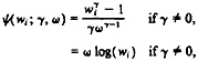
(1)
where ω is the geometric mean, of the observations w1, . . . . wn.
By “transformed-normal distribution,” we mean that for some unknown values of γ and ω, the transformed observations ψ(wi; γ, ω) (i = 1, . . ., n) are normally distributed. Although the sample geometric mean is determined by the data, we will soon turn to a setting involving a mixture of two components with different transformations to normality, in which even the sample geometric means of the two components are unknown; consequently, we treat a as an unknown parameter, the population geometric mean.
When the transformations are not scaled by the geometric-mean factor, as Box and Cox (1964, p. 217) noted, “the general size and range of the transformed observations may depend strongly on [γ].” Of considerable interest in our setting is that when transformations are scaled, not only are the likelihoods for different values of γ directly comparable, at least asymptotically, but also, by implication, so are the residual sums of squares on the transformed scales for different values of γ. In other words, scaling the transformations by ωγ−1 has the effect asymptotically of unconfounding the estimated variance on the transformed scale from the estimated power parameter. This result is important in the context of fitting mixtures of transformed-normal distributions when putting constraints on component variances in the fitting of the mixture model; by using scaled transformations, we can constrain the variance ratio without reference to the specific power transformation that has been applied to the data
Box and Cox (1964) also considered an unknown location parameter in the transformation, which may be needed because power transformations are defined only for positive random variables. Because the weights that arise from recordlinkage procedures are often allowed to be negative, this issue is relevant in our application. Nevertheless, Belin (1991) reported acceptable results using an ad hoc linear transformation of record-linkage weights to a range from 1 to 1,000. Although this ad hoc shift and rescaling is assumed to be present, we suppress the parameters of this transformation in the notation.
In the next section we outline in detail a transformed-normal mixture model for record-linkage weights. Fitting this model requires separate estimates of γ and ω for the true-match and false-match distributions observed in the training data, as well as an estimate of the ratio of variances on the transformed scale. The γ's can, as usual, be estimated by performing a grid search of the likelihoods or of the respective posterior densities. A modal estimate of the variance ratio can be obtained as a by-product of the estimation of the γ's. We also obtain approximate large-sample variances by calculating for each parameter a second difference as numerical approximation to the second derivative of the loglikelihood in the neighborhood of the maximum (Belin 1991). In our work we have simply fixed the ω's at their sample values, which appeared to be adequate based on the overall success of the methodology on both real and simulated data; were it necessary to obtain a better fit to the data, this approach could be modified.
2.3 Fitting Transformed Normal Mixtures with Fixed Global Parameters
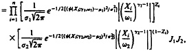
2.3.1 Background on Fitting Normal Mixtures Without Transformations. Suppose that f1 and f2 are densities that depend on an unknown parameter φ, and that the density f is a mixture of f1 and f2, i.e., f(X|φ, λ), = λf1(X|φ) + (1 − λ) f2(X|φ) for some λ between 0 and 1. Given an iid sample (X1, X2. . . , Xn) from f(X|φ, λ), the likelihood of θ = (φ, λ) can then be written as
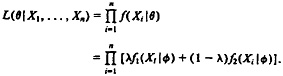
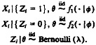
Following the work of many authors (e.g.. Aitkin and Rubin 1985; Dempster et al. 1977; Little and Rubin 1987; Orchard and Woodbury 1972; Titterington et al. 1985), we formulate the mixture model in terms of unobserved indicators of component membership Zi, i = 1, ..., n, where Zi = 1 if Xi comes from component 1 and Zi = 0 if Xi comes from component 2. The mixture model can then be expressed as a hierarchical model,
The “complete-data” likelihood, which assumes that the “missing data” Z1, . . . , Zn are observed, can be written as
L(φ, λ|X1, . . . , Xn; Z1, . . . , Zn)
Viewing the indicators for component membership as missing data motivates the use of the EM algorithm to obtain MLE's of (φ, λ). The E step involves finding the expected value of the Zi's given the data and current parameter estimates φ(t) and λ(t), where t indexes the current iteration. This is computationally straightforward both because the iid structure of the model implies that Zi is conditionally independent of the rest of the data given Xi and because the Zi's are indicator variables, so the expectation of Zi is simply the posterior probability that Zi equals 1. Using Bayes's theorem, the E step at the (t + 1)st iteration thus involves calculating
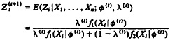
(2)
for i = 1, . . . , n.
The M step involves solving for MLE's of θ in the “complete-data” problem. In the case where f1 corresponds to the ![]() distribution and f2 corresponds to the
distribution and f2 corresponds to the ![]()
![]() distribution, so that
distribution, so that ![]() the M step at
the M step at
iteration (t + 1) involves calculating
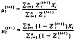
(3)
and
(4)
The updated value of λ at the (t + 1)st iteration is given by
(5)
which holds no matter what the form of the component densities may be. Instabilities can arise in maximum likelihood estimation for normally distributed components with distinct variances, because the likelihood is unbounded at the boundary of the parameter space where either ![]() Unless the starting values for EM are near a local maximum of the likelihood, EM can drift toward the boundary where the resulting fitted model suggests that one component consists of any single observation (with zero variance) and that the other component consists of the remaining observations (Aitkin and Rubin 1985).
Unless the starting values for EM are near a local maximum of the likelihood, EM can drift toward the boundary where the resulting fitted model suggests that one component consists of any single observation (with zero variance) and that the other component consists of the remaining observations (Aitkin and Rubin 1985).
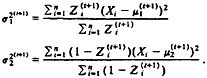
When a constraint is placed on the variances of the two components, EM will typically converge to an MLE in the interior of the parameter space. Accordingly, a common approach in this setting is to find a sensible constraint on the variance ratio between the two components or to develop an informative prior distribution for the variance ratio. When the variance ratio ![]() is assumed fixed, the E step proceeds exactly as in (2) and the M step for
is assumed fixed, the E step proceeds exactly as in (2) and the M step for ![]() and
and ![]() is given by (3); the M step for the scale parameters with fixed V is
is given by (3); the M step for the scale parameters with fixed V is

(6)
2.3.2 Modifications to Normal Mixtures for Distinct Transformations of the Two Components. We now describe EM algorithms for obtaining MLE's of parameters in mixtures of transformed-normal distributions, where there are distinct transformations of each component. Throughout the discussion, we will assume that there are exactly two components; fitting mixtures of more than two components involves straightforward extensions of the arguments that follow (Aitkin and Rubin 1985).
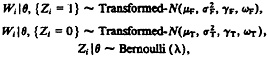
We will also assume that the transformations are fixed; that is, we assume that the power parameters (the two γi's) and the “geometric-mean” parameters (the two ωi's) are known in advance and are not to be estimated from the data. We can write the model for a mixture of transformed-normal components as follows:
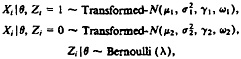
where ![]() and the expression “Transformed-N” with four arguments refers to the transformed-normal distribution with the four arguments being the location, scale, power parameter, and “geometric-mean” parameter of the transformed-normal distribution. The complete-data likelihood can be expressed as
and the expression “Transformed-N” with four arguments refers to the transformed-normal distribution with the four arguments being the location, scale, power parameter, and “geometric-mean” parameter of the transformed-normal distribution. The complete-data likelihood can be expressed as
L(θ|X1, . . . , Xn; Z1, . . . , Zn)
where J1 and J2 are the Jacobians of the scaled transformations X → ψ. If ω1 and ω2 were not fixed a priori but instead were the geometric means of the Xi for the respective components, then J1 = J2 = 1. In our situation, however, because the Zi's are missing, J1 and J2 are functions of {Xi}, {Zi}, and θ, and are not generally equal to 1. Still, J1 and J2 are close to 1 when the estimated geometric mean of the sample Xi in component k is close to ωk. We choose to ignore this minor issue; that is, although we model ω1 and ω2 as known from prior considerations, we still assume J1 = J2 = 1. To do otherwise would greatly complicate our estimation procedure with, we expect, no real benefit; we do not blindly believe such fine details of our model in any case, and we would not expect our procedures to be improved by the extra analytic work and computational complexity.
To keep the distinction clear between the parameters assumed fixed in EM and the parameters being estimated in EM, we partition the parameter into ![]() where
where ![]() and
and ![]() and where the variance ratio
and where the variance ratio ![]() Based on this formulation, MLE's of
Based on this formulation, MLE's of ![]() can be obtained from the following EM algorithm:
can be obtained from the following EM algorithm:
E step. For i = 1, . . ., n, calculate ![]() as in (2), where
as in (2), where
(7)
M step. Calculate![]() and
and ![]() as in (3), λ(t+1) as in (5), and
as in (3), λ(t+1) as in (5), and ![]() and
and ![]() as in (6), with Xi replaced by ψ(Xi; γg, ωg) for g = 1, 2; if the variance ratio V were not fixed but were to be estimated, then (4) would be used in place of (6).
as in (6), with Xi replaced by ψ(Xi; γg, ωg) for g = 1, 2; if the variance ratio V were not fixed but were to be estimated, then (4) would be used in place of (6).
2.3.3 Transformed-Normal Mixture Model for Record-Linkage Weights. Let the weights associated with record pairs in a current data set be denoted by Wi,i = 1, . . . , n,
where as before Zi = 1 implies membership in the false-match component and Zi = 0 implies membership in the true-match component. We assume that we have already obtained, from a training sample, (a) values of the power transformation parameters, denoted by γF for the false-match component and by γT for the true-match component, (b) values of the “geometric mean” parameters in the transformations, denoted by ωF for the false-match component and by ωT for the true-match component, and (c) a value for the ratio of the variances between the false-match and true-match components, denoted by V. Our model then becomes
where ![]() . We work with
. We work with ![]() and
and ![]()
![]() The algorithm of Section 2.3.2, with “F” and “T” substituted for “1” and “2,” describes the EM algorithm for obtaining MLE's of
The algorithm of Section 2.3.2, with “F” and “T” substituted for “1” and “2,” describes the EM algorithm for obtaining MLE's of ![]() from {Wi; i = 1, . . . , n} with {Zi; i = 1, . . . , n} missing and global parameters γF, γT, ωF, ωT, and V fixed at specified values.
from {Wi; i = 1, . . . , n} with {Zi; i = 1, . . . , n} missing and global parameters γF, γT, ωF, ωT, and V fixed at specified values.
2.4 False-Match Rate Estimates and Standard Errors with Fixed Global Parameters
2.4.1 Estimates of the False-Match Rate. Under the transformed-normal mixture model formulation, the false-match rate associated with a cutoff C can be expressed as a function of the parameters θ as

(8)
Substitution of MLE's for the parameters in this expression provides a predicted false-match rate associated with cutoff C.
Because there is a maximum possible weight associated with perfect agreement in most record-linkage procedures, one could view the weight distribution as truncated above. According to this view, the contribution of the tail above the upper truncation point (say, B), should be discarded by substituting Φ([ψg(B; γg, ωg,) − μg]/σg) for the 1s inside the bracketed expressions (g = F, T as appropriate). Empirical investigation suggests that truncation of the extreme upper tail makes very little difference in predictions. The results in Sections 3 and 4 reflect false-match rate predictions without truncation of the extreme upper tail.
2.4.2 Obtaining an Asymptotic Covariance Matrix for Mixture-Model Parameters From SEM Algorithm. The SEM algorithm (Meng and Rubin 1991) provides a method for obtaining standard errors of parameters in models that are fit using the EM algorithm. The technique uses estimates of the fraction of missing information derived from successive EM iterates to inflate the complete-data variance-covariance matrix to provide an appropriate observed-data variance-covariance matrix. Details on the implementation of the SEM algorithm in our mixture-model setting are deferred to the Appendix.
Standard arguments lead to large-sample standard errors for functions of parameters. For example, the false-match rate e(C|θ) can be expressed as a function of the four components of ![]() by substituting for
by substituting for ![]() σT in (8). Then the squared standard error of the estimated false-match rate is given by SE2(e) ≈ dT Ad, where A is the covariance matrix for
σT in (8). Then the squared standard error of the estimated false-match rate is given by SE2(e) ≈ dT Ad, where A is the covariance matrix for ![]() obtained by SEM and the vth component of d is
obtained by SEM and the vth component of d is ![]()
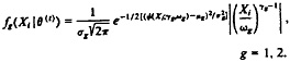
2.4.3 Estimates of the Probability of False Match for a Record Pair With a Given Weight. The transformed-normal mixture model also provide a framework far estimating the probability of false match associated with various cutoff weights. To be clear, we draw a distinction between the “probability of false match” and what we refer to as the “neighborhood false-match rate” to avoid any confusion caused by (1) our using a continuous mixture distribution to approximate the discrete distribution of weights associated with a finite number of record pairs, and (2) the fact that there are only finitely many possible weights associated with many record-linkage weighting schemes. The “neighborhood false-match rate around W” is the number of false matches divided by the number of declared matches among pairs of records with composite weights in a small neighborhood of W; with a specific model, the neighborhood false-match rate is the “probability of false match” implied by the relative density of the true-match and false-match components at W.
In terms of the mixture-model parameters, the false-match rate among record pairs with weights between W and W + h is given by
where
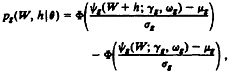
g=F, T,
and ![]() . Although the number of false matches is not a smooth function of the number of declared matches, ξ(W, h|θ) is a smooth function
. Although the number of false matches is not a smooth function of the number of declared matches, ξ(W, h|θ) is a smooth function
of h. The probability of false match under the transformed-normal mixture model is the limit as h→ 0 of ξ(W, h|θ), which we denote as η(W|θ); we obtain
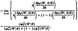
(9)
where
g = F, T.
Estimates of neighborhood false-match rates are thus routinely obtained by substituting the fixed global parameter values and MLE's of μF, μT, σF, σT, and λ into (9).
Because the neighborhood false-match rate captures the trade-off between the number of false matches and the number of declared matches, the problem of setting cutoffs can be cast in terms of the question “Approximately how many declared matches are needed to make up for the cost of a false match?” If subject matter experts who are using a record-linkage procedure can arrive at an answer to this question, then a procedure for setting cutoffs could be determined by selecting a cutoff weight where the estimated neighborhood false-match rate equals the appropriate ratio. Alternatively, one could monitor changes in the neighborhood false-match rate (instead of specifying a “tolerable ” neighborhood false-match rate in advance) and could set a cutoff weight at a point just before the neighborhood false-match rate accelerates.
2.5 Reflecting Uncertainty in Global Parameters
When there is more than one source of training data, the information available about both within-site and between-site variability in global parameters can be incorporated into the prior specification. For example, with two training sites, we could combine the average within-site variability in a global parameter with a 1 df estimate of between-site variability to represent prior uncertainty in the parameter. With many sites with covariate descriptors, we could model the multivariate regression of global parameters on covariates.
The procedure we used in the application to census/PES data offers an illustration in the simple case with two training sites available to calibrate a third site. For each of the training-data sites and each of the components (true-match and false-match), joint MLE's were found for ![]() g = F, T, using a simple grid-search over the power parameters. This yielded two estimates of the power parameters, γF and γT, and two estimates of the variance ratio V between the false-match and true-match components. Additionally, an estimated variance-co variance matrix for these three parameters was obtained by calculating second differences of the loglikelihood at grid points near the maximum.
g = F, T, using a simple grid-search over the power parameters. This yielded two estimates of the power parameters, γF and γT, and two estimates of the variance ratio V between the false-match and true-match components. Additionally, an estimated variance-co variance matrix for these three parameters was obtained by calculating second differences of the loglikelihood at grid points near the maximum.
Values of each parameter for the mixture-model fitting were drawn from separate truncated-normal distributions with mean equal to the average of the estimates from the two training sites and variance equal to the sum of the squared differences between the individual site parameter values and their mean (i.e., the estimated “between ” variance), plus the average squared standard error from the two prior fittings (i.e., the average “within” variance). The truncation ensured that the power parameter for the false-match component was less than i, that the power parameter for the true-match component was greater than 1, and that the variance ratio was also greater than 1. These constraints on the power parameters were based on the view that because there is a maximum possible weight corresponding to complete agreement and a minimum possible weight corresponding to complete disagreement, the true-match component will have a longer left tail than right tail and the false-match component will have a longer right tail than left tail. The truncation for the variance ratio was based on an assumption that false-match weights will exhibit more variability than true-match weights for these data on the transformed scale as well as on the original scale.
For simplicity, the geometric-mean terms in the transformations ( ωF and ωT) were simply fixed at the geometric mean of the component geometric means from the two previous sites. If the methods had not worked as well as they did with test and simulated data, then we would have also reflected uncertainty in these parameters.
Due to the structure of our problem, in which the role of the prior distribution is to represent observable variability in global parameters from training data, we presume that the functional form of the prior is not too important as long as variability in global parameters is represented accurately. That is, we anticipate that any one of a number of methods that reflect uncertainty in the parameters estimated from training data will yield interval estimates with approximately the correct coverage properties, i.e., nominal (1 − α) × 100% interval estimates will cover the true value of the estimand approximately (1 − α) × 100% or more of the time. Alternative specifications for the prior distribution were described by Belin (1991).
When we fit multiple mixture models to average over uncertainty in the parameters estimated by prior data (i.e., when we use the “full strategy” of Section 2.1), the multiple-imputation framework of Rubin (1987) can be invoked to combine estimates and standard errors from the separate models to provide one inference. Suppose that we fit m mixture models corresponding to m separate draws of the global parameters from their priors and thereby obtain false-match rate estimates e1, e2, . . . , em and variance estimates u1, u2, . . . , um, where u1 = SE2 (e1) is obtained by the method of Section 2.4.2. Following Rubin (1987, p. 76), we can estimate the false-match rate by
and its squared standard error by
Monte Carlo evaluations documented by Rubin (1987, secs. 4.6–4.8) illustrate that even a few imputations (m = 2, 3, or 5) are enough to produce very reasonable coverage properties for interval estimates in many cases. The combination of estimation procedures that condition on global parameters with a multiple-imputation procedure to obtain inferences that average over those global parameters is a powerful technique that can be applied quite generally.
3. PERFORMANCE OF CALIBRATION PROCEDURE ON CENSUS COMPUTER-MATCHING DATA
3.1 Results From Test-Census Data
We use the test-census data described in Section 1.3 to illustrate the performance of the proposed calibration procedure, where determinations by clerks are the best measures available for judging true-match and false-match status. With three separate sites available, we were able to apply our strategy three times, with two sites serving as training data and the mixture-model procedure applied to the data from the third site.
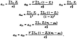
We display results from each of the three tests in Figure 2. The dotted curve represents predicted false-match rates obtained from the mixture-model procedure, with accompanying 95% intervals represented by the dashed curves. Also plotted are the observed false-match rates, denoted by the “O” symbol, associated with each of several possible choices of cutoff values between matches and nonmatches.
We call attention to several features of these plots. First, it is clearly possible to match large proportions of the files with little or no error. Second, the quality of candidate matches becomes dramatically worse at some point where the false-match rate accelerates. Finally, the calibration procedure performs very well in all three tests from the standpoint of providing predictions that are close to the true values and interval estimates that include the true values.
In Figure 3 we take a magnifying glass to the previous displays to highlight the behavior of the calibration procedure in the region of interest where the false-match rate accelerates. That the predicted false-match rate curves bend upward close to the points where the observed false-match rate curves rise steeply is a particularly encouraging feature of the calibration method.
For comparison with the logistic-regression approach, we report in Table 2 (p. 704) the estimated false-match rates across the various sites for records with weights in the interval [−5, 0], which in practice contains both true matches and false matches. Two alternative logistic regression models— one in which logit(η) is modeled as a linear function of matching weight and the other in which logit(η) is modeled as a quadratic function of matching weight, where η is the probability of false match—were fitted to data from two sites to predict false-match rates in the third site. A predictive standard error to reflect binomial sampling variability, as well as uncertainty in parameter estimation, was calculated using
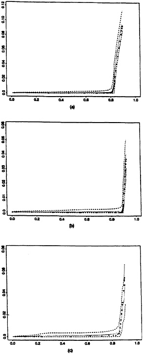
Figure 2. Performance of Calibration Procedure on Test-Census Data: (a) St. Louis, Using Columbia and Washington as Training Sample; (b) Columbia, Using St. Louis and Washington as Training Sample; (c) Washington. Using St. Louis and Columbia as Training Sample. O = observed false-match rate; . . . = predicted false-match rate; . . . = upper and lower 95% bounds.
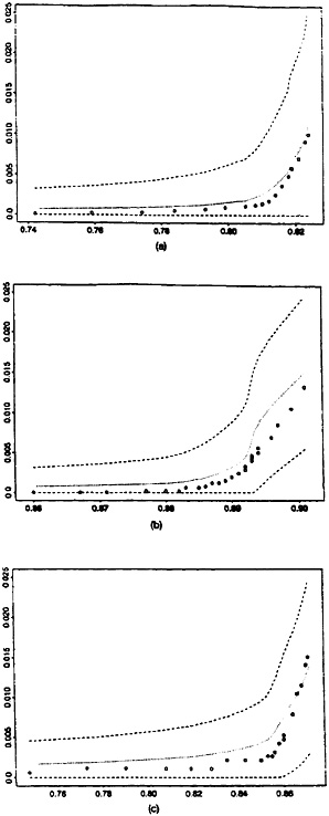
Figure 3. Performance of Calibration Procedure in Region of Interest: (a) St. Louis, Using Columbia and Washington as Training Sample; (b) Columbia, Using St. Louis and Washington as Training Sample; (c) Washington, Using St. Louis and Columbia as Training Sample. O = observed false-match rate; = predicted false-match rate; - - - = upper and lower 95% bounds.
where n* is the number of record pairs with weights in the target interval and ![]() is the predicted probability of false match for candidate pair i. For the linear logistic model, we have wi = (1, wi)T, where wi is the weight for record pair i and var
is the predicted probability of false match for candidate pair i. For the linear logistic model, we have wi = (1, wi)T, where wi is the weight for record pair i and var ![]() is the 2 × 2 covariance matrix of the regression parameters, whereas for the quadratic logistic model we have
is the 2 × 2 covariance matrix of the regression parameters, whereas for the quadratic logistic model we have ![]() where var
where var ![]() is the 3 × 3 covariance matrix of the regression parameters.
is the 3 × 3 covariance matrix of the regression parameters.
As can be seen from Table 2, the predicted false-match rates from two alternative logistic regression models often were not in agreement with the observed false-match rates; in fact, they were often several standard errors apart. Because weights typically depend on site-specific data, this finding was not especially surprising. It is also noteworthy that the estimate of the quadratic term ß2 in the quadratic models was more than two standard errors from zero using the St. Louis data (p = 029) but was near zero using the Columbia and Washington data sets individually (p = 928 and p = 719). Using the mixture-model calibration approach, in two of the three sites the observed false-match rate is within two standard errors of the predicted false-match rate, and in the other site (St. Louis) the mixture-model approach is conservative in that it overstates the false-match rate. We regard this performance as superior to that of logistic regression—not surprising in light of our earlier discussion in Section 1.3 of why we eschewed logistic regression in this setting. Refining the mixture-model calibration approach through a more sophisticated prior distribution for global parameters (e.g., altering the prior specification so that urban sites are exchangeable with one another but not with rural sites) may result in even better performance by reflecting key distinctions in distributional shapes across sites.
3.2 A Limitation in the Extreme Tails
For small proportions of the records declared matched, counter-intuitive false-match rate estimates arise, with false-match rate estimates increasing as the proportion declared matched goes to zero. Such effects are explained by the false-match component being more variable than the true-match component, so that in the extreme upper tail of the component distributions the false-match component density is greater than the true-match component density. To avoid nonsensical results (since we know that the false-match rate should go to zero as the weight approaches the maximum possible weight), we find the points along the false-match-rate curve and the upper interval-estimate curve, if any, where the curves depart from a monotone decreasing pattern as the proportion declared matched approaches zero. From the point at which the monotone pattern stops, we linearly interpolate false-match rate estimates between that point and zero. We are not alarmed to find that the model does not fit well in the far reaches of the upper tails of component distributions, and other smoothing procedures may be preferred to the linear-interpolation procedure used here.
Table 2. Performance of Mixture-Model Callibration Procedure on Test-census Matching Weights in the interval [−5, 0]
|
Site to be predicted |
Observed false-match rate among cases with weights in [−5, 0] |
Predicted false-match rate (SE) for cases with weights in [−5, 0] under linear logistic model; that is logit(η) = α + β (Wt) |
Predicted false-match rate (SE) for cases with weights in [−5, 0] under quadratic logistic model; that is logit(η) = α + β, (Wt) + β2(Wt)2 |
Predicted false-match rate (SE) for cases with weights in [−5, 0] based on mixture-model calibration method |
|
St. Louis |
.646 |
.417 |
.429 |
.852 |
|
(=73/113) |
(.045) |
(.045) |
(.033) |
|
|
Columbia |
.389 |
.584 |
.613 |
.524 |
|
(= 14/36) |
(.079) |
(.079) |
(.083) |
|
|
Washington |
.294 |
.573 |
.597 |
.145 |
|
(= 5/17) |
(.115) |
(.115) |
(.085) |
4. SIMULATION EXPERIMENT TO INVESTIGATE PROPERTIES OF CALIBRATION PROCEDURE
4.1 Description of Simulation Study
Encouraged by the success of our method with real data, we conducted a large simulation experiment to enhance our understanding of the calibration method and to study statistical properties of the procedure (e.g., bias in estimates of the false-match rate, bias in estimates of the probability of false match, coverage of nominal 95% interval estimates for false-match rates, etc.) when the data generating mechanism was known. The simulation procedure involved generating data from two overlapping component distributions, with potential “site-to-site ” variability from one weight distribution to another, to represent plausible weights, and replicating the calibration procedure on these samples.
Beta distributions were used to represent the components of the distribution of weights in the simulation experiment Simulated weights thus were generated from component distributions that generally would be skewed and that have a functional form other than the transformed-normal distribution used in our procedure. The choice of beta-distributed components was convenient in that simple computational routines were available (Press, Flannery, Teukolsky, and Vetterling 1986) to generate beta-random deviates and to evaluate tail probabilities of beta densities.
Table 3 lists factors and outcome variables that were included in the experiment Here we report only broad descriptive summaries from the simulation study. Greater detail on the design of the experiment and a discussion of the strategy for relating simulation outcomes to experimental factors have been provided by Belin (1991). The calibration procedure was replicated 6,000 times, with factors selected in a way that favored treatments that were less costly in terms of computer time (for details, again see Belin 1991).
4.2 Results
Figure 4 displays the average relative bias from the various simulation replicates in a histogram. Due to the way that we have defined relative bias (see Table 3), negative values correspond to situations where the predicted false-match rate is greater than the observed false-match rate; that is, negative relative bias corresponds to conservative false-match rate estimates. It is immediately apparent that the calibration procedure is on target in the vast majority of cases, with departures failing mostly on the “conservative” side, where the procedure overstates false-match rates and only a few cases where the procedure understates false-match rates.
The few cases in which the average relative bias was unusually large and negative were examined more closely, and all of these had one or more cutoffs where the observed false-match rate was zero and the expected false-match rate was small. In such instances the absolute errors are small, but relative errors can be very large. Clearly, however, errors between a predicted false-match rate of .001 or .002 and observed false-match rate of 0 presumably are not of great concern in applications.
There was a single replicate that had a positive average relative bias substantially larger than that of the other replicates. Further investigation found that a rare event occurred in that batch, with one of the eight highest-weighted records being a false match, which produced a very high relative error. In this replicate, where the predicted false-match rate under the mixture model was .001, the observed false-match rate was .125 and the expected (beta) false-match rate was .00357. Belin (1991) reported that other percentiles of the distribution in this replicate were fairly well calibrated (e.g., predicted false-match rates of .005, .01, .10, .50, and .90 corresponded to expected beta false-match rates of .007, .011, .130, .455, and .896); thus it was apparently a rare event rather than a breakdown in the calibration method that led to the unusual observation.
With respect to the coverage of interval estimates, we focus on simulation results when the SEM algorithm was applied to calculate a distinct covariance matrix for each fitted mixture model (n = 518). In the other simulation replicates, shortcuts in standard error calculations were taken so as to avoid computation; Belin (1991) reported that these shortcut methods performed moderately worse in terms of coverage. For nominal two-sided 95% intervals, the calculated intervals covered observed false-match rates 88.58% of the time (SE = 1.94%); for nominal one-sided 97.5% intervals, the calculated intervals covered observed false-match rates 97.27% of the time (SE = 1.45%). Thus the calibration method does not achieve 95% coverage for two-sided interval estimates, but when it errs it tends to err on the side of overstating false-match rates, so that the one-sided interval estimates perform well.
Table 3. Description of Factors and Outcomes in Simulation
|
Experimental factors |
Comments |
|
1. Possible values = {3, 4, 30} 2–3. Possible values = {2,000, 2,001, 9,999} 4. Possible values in [.01, 5] 5. Be(aF, bF),aF ~ U(1.75, 2) bF ~ U(3, 6). 6. Be(aT, bT), aT ~ U(8, 12) bT ~ U(1.75, 2) 7–8. Separate draws from 5–8 for separate sites, or common shapes across sites 9. Perform SEM for each mixture model being fit, or a short-cut method to save computing time based on approximations 10. Possible values = {3, 5, 10} |
|
Outcomes measured in simulation |
Comments |
|
1. Prespecified false-match rates = {.001, 002, 015, 02, 025, 03, 04, 05} Relative bias = [(observed false-match rate) - (predicted false- match rate)]/v(expected false-match rate) “predicted false-match rate” = estimated false-match rate calculated under transformed-normal mixture model “observed false-match rate” = {# false matches}/{# declared matches} at given cutoff “expected false-match rate” = {tail area of Beta false-match component}/(sum of tail areas of Beta component distributions} 2–3. Same prespecified false-match rates as in 1. 4. Estimated probabilities of false match = {.00125, 0025, 005, 01, 02, 10, 25, 50, 75, 90} |
Turning to the performance of the estimated probabilities of false match (i.e., neighborhood false-match rates) obtained from the fitted mixture models, Table 4 provides the mean, standard deviation, minimum, and maximum of the true underlying probabilities being estimated by the calibration procedure. Although in specific sites the calibration procedure substantially understates or overstates false-match rates, the procedure appears to have good properties in the aggregate.
5. DISCUSSION
Previous attempts at estimating false-match rates in record linkage were either unreliable or too cumbersome for practical
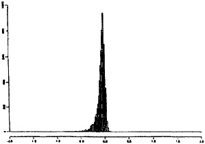
Figure 4. Histogram of Average Relative Bias Across Simulation Replicates.
use. Although our method involves fitting nonstandard models, other researchers have used software that we developed to implement the technique in at least two other settings (Ishwaran, Berry, Duan, and Kanouse 1991; Scheuren and Winkler 1991, 1993). This software is available on request from the first author.
Analyses by Belin (1991) have revealed that the deficiencies in the calibration procedure typically occurred where the split in the proportion of records between the two components was very extreme. For example, after excluding a few dozen replicates where 99% or more of the records were declared matched above the point where the procedure predicted a false-match rate of 005, there was no evidence that sample sizes of the data bases being matched had an impact on the accuracy of estimated probabilities of false match, implying that breakdown of the calibration procedure appears to be a threshold phenomenon.
Table 4. Performance of Estimated Probabilities of False-Match in Predicting True Underlying Probabilities
|
Estimated probability |
Mean of actual probabilities |
Std. deviation of actual probabilities |
Minimum of actual probabilities |
Maximum of actual probabilities |
|
.00125 |
.00045 |
.00075 |
.00000 |
.0105 |
|
.0025 |
.0012 |
.00143 |
.00000 |
.0170 |
|
.005 |
.0030 |
.00266 |
.00000 |
.0295 |
|
.01 |
.0072 |
.00470 |
.00002 |
.059 |
|
.02 |
.0160 |
.00818 |
.00019 |
.1183 |
|
.10 |
.0813 |
.03231 |
.00155 |
.4980 |
|
.25 |
.2066 |
.07385 |
.00549 |
.8094 |
|
.50 |
.4555 |
.11996 |
.02812 |
.9551 |
|
.75 |
.7459 |
.10768 |
.20013 |
.9988 |
|
.90 |
.9244 |
.05222 |
.56845 |
1.000 |
Finally, on several occasions when we have discussed these techniques and associated supporting evidence, we have been questioned about the validity of using determinations of clerks as a proxy for true-match or false-match status. Beyond pointing to the results of the simulations, we note that (a) clerical review is as close to truth as one is likely to get in many applied contexts, and (b) possible inaccuracy in assignment of match status by clerks is no criticism of the calibration procedure. This methodology provides a way to calibrate false-match rates to whatever approach is used to identify truth and falsehood in the training sample and appears to be a novel technique that is useful in applied contexts.
APPENDIX: IMPLEMENTATION OF THE SEM ALGORITHM
The SEM algorithm is founded on the identity that the observed data observed information matrix ![]() for a k-dimensional perameter θ can be expressed in terms of the conditional expectation of the “complete-data” observed information matrix evaluated at the MLE
for a k-dimensional perameter θ can be expressed in terms of the conditional expectation of the “complete-data” observed information matrix evaluated at the MLE ![]() as
as
where I is the k × k identity matrix and DM is the Jacobian of the mapping defined by EM (i.e., of the mapping that updates parameter values on the tth iteration to those on the (t + 1)st iteration) evaluated at the MLE ![]() . Taking inverses of both sides of the previous equation yields the identity
. Taking inverses of both sides of the previous equation yields the identity
where ![]() and ∆V=Vcom DM(I − DM)−1, the latter reflecting the increase in variance due to the missing information.
and ∆V=Vcom DM(I − DM)−1, the latter reflecting the increase in variance due to the missing information.
The SEM procedure attempts to evaluate the DM matrix of partial derivatives numerically. First, EM is run to convergence and the MLE ![]() is obtained. To compute partial derivatives, all but one of the components of the parameter are fixed at their MLE's, and the remaining component is set to its value at the tth iteration, say θ(t)(i). Then, after taking a “forced EM step” by using this parameter value as a start to a single iteration ( E step and M step), the new estimates, say
is obtained. To compute partial derivatives, all but one of the components of the parameter are fixed at their MLE's, and the remaining component is set to its value at the tth iteration, say θ(t)(i). Then, after taking a “forced EM step” by using this parameter value as a start to a single iteration ( E step and M step), the new estimates, say ![]() for j=1, . . . , k, yield the following estimates of partial derivatives:
for j=1, . . . , k, yield the following estimates of partial derivatives:
It is necessary to perform k forced EM steps at every iteration of SEM—although Meng and Rubin (1991) pointed out that once convergence is reached for each component of the vector (ri,1, ri,2, . . . , ri, k), it is no longer necessary to perform the forced EM step for component i = i′.
Because we regard the variance ratio as fixed when fitting our mixture models, we are actually estimating four parameters in the calibration mixture-model setting: the locations of the two components, one unknown scale parameter, and a mixing parameter. We can calculate the complete-data information matrix for ![]()
![]() as
as
where
The missing information in our problem arises from the fact that the Zi's are unknown.
Because the covariance matrix is 4 × 4, every iteration or the SEM algorithm takes roughly four times as long as an iteration of EM. It also should be pointed out that the SEM algorithm relies on precise calculation of MLE's. Although it may only be necessary to run EM for 10 or 20 iterations to obtain accuracy to two decimal places in MLE's, it might take 100 or more iterations to obtain accuracy to, say, six decimal places. These aspects of the SEM algorithm can make it computationally expensive.
The DM matrix containing the rv’s will not generally be symmetric, but of course the resulting covariance matrix should be symmetric. If the resulting covariance matrix is not symmetric even though several digits of numerical precision are obtained for the MLE and the rv’s, this reflects an error in the computer code used to implement the forced SEM steps or perhaps in the code for the resulting covariance matrix thus provides a diagnostic check on the correctness of the program.
Experience with the SEM algorithm suggests that convergence of the numerical approximations to the partial derivatives of the mapping often occurs in the first few iterations and further reveals that beyond a certain number of iterations, the approach can give nonsensical results owing to limitations in numerical precision, just as with any numerical differentiation procedure. Meng and Rubin (1991) suggested specifying a convergence criterion for the rv’s and ceasing to calculate these terms once the criterion is satisfied for all j = 1, . . ., k. An alternative (used in producing the results in Secs. 3 and 4) involves running the SEM algorithm for eight iterations, estimating an partial derivatives of the mapping on each iteration, assessing which two of the eight partial derivative estimates are closest to one another, and taking the second of the two as our estimate of the derivative. Experience with this approach suggests that it yields acceptable results for practice in that the off-diagonal elements of the resulting covariance matrix agree with one another to a few decimal places.
[Received February 1993. Revised November 1993.]
REFERENCES
Aitkin, M., and Rubin, D.B. ( 1985), “Estimation and Hypothesis Testing in Finite Mixture Models,” Journal of the Royal Statistical Society, Ser. B, 47, 67–75.
Belin, T.R. ( 1989a), “Outline of Procedure for Evaluating Computer Matching in a Factorial Experiment,” unpublished memorandum, U.S. Bureau of the Census, Statistical Research Division.
—— ( 1989b), “Results from Evaluation of Computer Matching,” unpublished memorandum, U.S. Bureau of the Census, Statistical Research Division.
—— ( 1990), “A Proposed Improvement in Computer Matching Techniques,” in Statistics of Income and Related Administrative Record Research: 1988–1989. Washington, DC U.S. Internal Revenue Service, pp. 167–172.
—— ( 1991), “Using Mixture Models to Calibrate Error Rates in Record-Linkage Procedures, with Application to Computer Matching for Census Undercount Estimation, ” Ph.D. thesis, Harvard University, Dept. of Statistics.
Box, G.E.P., and Cox, D.R. ( 1964), “An Analysis of Transformations” (with discussion), Journal of the Royal Statistical Society, Ser. B, 26, 206–252.
Brown, P., Laplant, W., Lynch, M., Odell, S., Thibaudeau, Y., and Winkler, W. ( 1988), Collective Documentation for the 1988 PES Computer-Match Processing and Printing. Vols. I–III, Washington, DC: U.S. Bureau of the Census, Statistical Research Division.
Copas, J., and Hilton, F. ( 1990), “Record Linkage: Statistical Models for Matching Computer Records, ” Journal of the Royal Statistical Society, Ser. A. 153, 287–320.
Dawid, A.P. ( 1976), “Properties of Diagnostic Data Distributions,” Biometrics, 32, 647–658.
Dempster, A.P., Laird, N.M., and Rubin, D.B. ( 1977), “Maximum Likelihood from Incomplete Data via the EM Algorithm” (with discussion), Journal of the Royal Statistical Society, Ser. B, 39, 1–38.
Efron, B. ( 1975), “The Efficiency of Logistic Regression Compared to Normal Discriminant Analysis,” Journal of the American Statistical Association, 70, 892–898.
Fellegi, I.P., and Sunter, A.B. ( 1969), “A Theory for Record Linkage,” Journal of the American Statistical Association, 64, 1183–1210.
Halperin, M., Blackwelder, W.C., and Verter, J.I. ( 1971), “Estimation of the Multivariate Logistic Risk Function: A Comparison of the Discriminant Function and Maximum Likelihood Approaches,” Journal of Chronic Diseases, 24, 125–158.
Hogan, H. ( 1992), “The 1990 Post-Enumeration Survey: An Overview,” The American Statistician, 46, 261–269.
Ishwaran, H., Berry. S., Duan, N., and Kanouse, D. ( 1991). “Replicate Interviews in the Los Angeles Women's Health Risk Study: Searching for the Three-Faced Eve,” technical report, RAND Corporation.
Jaro, M.A. ( 1989), “Advances in Record-Linkage Methodology as Applied to Matching the 1985 Census of Tampa, Florida,” Journal of the American Statistical Association, 84, 414–420.
Kelley, R.P. ( 1986). “Robustness of the Census Bureau's Record Linkage System,” in Proceedings of the American Statistical Association, Section on Survey Research Methods, pp. 620–624.
Little, R.J.A., and Rubin, D.B. ( 1987), Statistical Analysis with Missing Data, New York: John Wiley.
Maclean, C.J., Morton, N.E., Elston, R.C., and Yee, S. ( 1976), “Skewness in Commingled Distributions,” Biometrics, 32, 695–699.
Mantel, N., and Brown, C. ( 1974), “Alternative Tests for Comparing Normal Distribution Parameters Based on Logistic Regression,” Biometrics, 30 485–497.
Meng, X.L., and Rubin, D.B. ( 1991), “Using EM to Obtain Asymptotic Variance-Covariance Matrices: The SEM Algorithm,” Journal of the American Statistical Association, 86, 899–909.
Newcombe, H.B. ( 1988), Handbook of Record Linkage: Methods for Health and Statistical Studies, Administration, and Business, Oxford, U.K.: Oxford University Press.
Newcombe, H.B., Kennedy, J.M., Axford, S.J., and James. A.P. ( 1959), “Automatic Linkage of Vital Records,” Science, 130, 954–959.
Orchard, T., and Woodbury, M.A. ( 1972), “A Missing Information Principle: Theory and Applications,” Proceedings of the Sixth Berkeley Symposium on Mathematical Statistics and Probability. 1, 697–715.
Press, W.H., Flannery, B.P., Teukolsky, S.A., and Vetterling, W.T. ( 1986), Numerical Recipes: The Art of Scientific Computing, Cambridge, U.K.: Cambridge University Press.
Rogot, E., Sorlie, P.D., and Johnson, N.J. ( 1986), “Probabilistic Methods in Matching Census Samples to the National Death Index,” Journal of Chronic Diseases, 39, 719–734.
Rubin, D.B. ( 1987), Multiple Imputation for Nonresponse in Surveys, New York: John Wiley.
Scheuren, F., and Winkler, W.E. ( 1991), “An Error Model for Regression Analysis of Data Files That are Computer Matched,” in Proceedings of the 1991 Annual Research Conference, U.S. Bureau of the Census, pp. 669–687.
—— ( 1993). “Regression Analysis of data files that are computer matched,” Siney Methodology, 19, 39–58.
Tepping, B.J. ( 1968), “A Model for Optimum Linkage of Records,” Journal of the American Statistical Association, 63, 1321–1332.
Thibaudeau, Y. ( 1989), “Fitting Log-Linear Models in Computer Matching.” in Proceedings of the American Statistical Association, Section on Statis tical Computing, pp. 283–288.
Titterington, D.M., Smith, A.F.M., and Makov, U.E. ( 1985), Statistical Analysis of Finite Mixture Distributions, New York: John Wiley.
Weisberg, S. ( 1980), Applied Linear Regression, New York: John Wiley.
Winkler, W.E. ( 1989), “Near-Automatic Weight Computation in the Fellegi-Sunter Model of Record Linkage,” in Proceedings of the Fifth Annual Research Conference, U.S. Bureau of the Census, pp. 145–155.
Modeling Issues and the Use of Experience in Record Linkage
Michael D.Larsen, Harvard University
Abstract
The goal of record linkage is to link quickly and accurately records corresponding to the same person or entity. Fellegi and Sunter (1969) proposed a statistical model for record linkage that assumes pairs of entries, one from each of two files, either are matches corresponding to a single person or nonmatches arising from two different people. Certain patterns of agreements and disagreements on variables in the two files are more likely among matches than among non-matches. The observed patterns can be viewed as arising from a mixture distribution.
Mixture models, which for discrete data are generalizations of latent-class models, can be fit to comparison patterns in order to find matching and nonmatching pairs of records. Mixture models, when used with data from the U.S. Decennial Census—Post Enumeration Survey, quickly give accurate results.
A critical issue in new record-linkage problems is determining when the mixture models consistently identify matches and nonmatches, rather than some other division of the pairs of records. A method that uses information based on experience, identifies records to review, and incorporates clerically-reviewed data is proposed.
Introduction
Record linkage entails comparing records in one or more data files and can be implemented for unduplication or to enable analyses of relationships between variables in two or more files. Candidate records being compared really arise from a single person or from two different individuals. Administrative data bases are large and clerical review to find matching and nonmatching pairs is expensive in terms of human resources, money, and time. Automated linkage involves using computers to perform matching operations quickly and accurately.
Mixture models can be used when the population is composed of underlying and possibly unidentified subpopulations. The clerks manually identify matches and nonmatches, while mixture models can be fit to unreviewed data in the hopes of finding the same groups. However, mixture models applied to some variables can produce groups that fit the data but do not correspond to the desired divisions. A critical issue in this application is determining when the model actually is identifying matches and nonmatches.
A procedure is proposed in this paper that when applied to Census data seems to work well. The more that is known about a particular record linkage application, the better the procedure should work. The size of the two files being matched, the quality of the information recorded in the two files, and any clerical review that has already been completed are incorporated into the procedure. Additionally, the procedure
should help clerks be more efficient because it can direct their efforts and increase the value of reviewed data through use in the model.
The paper defines mixture models and discusses estimation of parameters, clustering, and error rates. Then previous theoretical work on record linkage is described. Next, the paper explains the proposed procedure. A summary of the application of the procedure to five Census data sets is given. The paper concludes with a brief summary of results and reiteration of goals.
Mixture Models
An observation yi (possibly multivariate) arising from a finite mixture distribution with G classes has probability density
p(yi|Π, Θ) = Σg=1,G πg pg(yi|θg), (1)
where πg (Σg=1,G πg =1), pg, and θg are the proportion, the density of observations, and the distributional parameters, respectively, in class g, and Π and Θ are abbreviated notation for the collections of proportions and parameters, respectively. The likelihood for π and θ based on a set of n observations is a product with index i=1,...,n of formula (1).
The variables considered in this paper are dichotomous and define a table of counts, which can have its cells indexed by i. In the application, each observation is ten dimensional, so n=1024. The mixture classes are in effect subtables, which when combined yield the observed table. The density pg(• | •) in mixture class g can be defined by a log-linear model on the expected counts in the cells of the subtable. The relationship among variables described by the log linear model can be the same or different in the various classes. When the variables defining the table in all classes are independent conditional on the class, the model is the traditional latent-class model. Sources for latent-class models include Goodman (1974) and Haberman (1974, 1979).
Maximum likelihood estimates of π and θ can be obtained using the EM (Dempster, Laird, Rubin 1977) and ECM (Meng and Rubin, 1993) algorithms. The ECM algorithm is needed when the log linear model in one or more of the classes can not be fit in closed form, but has to be estimated using iterative proportional fitting.
The algorithms treat estimation as a missing data problem. The unobserved data are the counts in each pattern in each class and can be represented by a matrix z with n rows and G columns, where entry zig is the number of observations with pattern i in class g. If the latent counts were known, the density would be
p(y, z|Π, Θ) = Πi=1,n Πg=1,G (πg pg(yi|θg))zig. (2)
Classified data can be used along with unclassified data in algorithms for estimating parameters. The density then is a combination of formulas (2) and a product over i of (1). Known matches and nonmatches, either from a previous similar matching problem or from clerk-reviewed data in a new problem, can be very valuable since subtables tend to be similar to the classified data.
Probabilities of group membership for unclassified data can be computed using Bayes' Theorem. For the kth observation in the ith cell, the probability of being in class g (zigk=1) is
p(zigk = 1 | yi, π, θ) = πg pg(yi | θg) / Σh=1,G πh ph(yi | θh). (3)
Probability (3) is the same for all observations in cell i. Probabilities of class membership relate to probabilities of being a match and nonmatch only to the degree that mixture classes are similar to matches and nonmatches.
The probabilities of group membership can be used to cluster the cells of the table by sorting the cells of the table according to descending probability of membership in a selected class. An estimated error rate at a given probability cut-off is obtained by dividing the expected number of observations not in a class by the total number of observations assigned to a class. As an error rate is reduced by assigning fewer cells to a class, the number of observations in a nebulous group not assigned to a class increases.
Before the match and nonmatch status is determined by clerks tentative declarations as probable match and probable nonmatch can be made using mixture models. It is necessary to choose a class or classes to be used as probable matches and probable nonmatches, which usually can be done by looking a probabilities of agreement on fields in the mixture classes. The estimated error rates from the mixture model correspond to the actual rate of misclassification of matches and nonmatches only to the degree that the mixture classes correspond to match and nonmatch groups.
Record Linkage Theory
Fellegi and Sunter (1969) proposed a statistical model for record linkage that assumes pairs of entries, one from each of two files, either are matches corresponding to a single person or nonmatches arising from two different people. Patterns of agreements and disagreements on variables have probabilities of occurring among matches and among nonmatches. If the pairs of records are ordered according to the likelihood ratio for being a match versus being a nonmatch and two cut-off points are chosen, one above which pairs are declared matches and one below which pairs are declared nonmatches, the procedure is optimal in the sense of minimizing the size of the undeclared set at given error levels.
Fellegi and Sunter (1969) suggested methods to estimate the unknown probabilities involved in the likelihood ratio. Some of their simplifying assumptions, such as the independence of agreement on fields of information within matches and nonmatches, have continued to be used extensively in applications.
In the methods proposed in this paper, the likelihood ratio is estimated using the mixture model. If the first class is the class of probable matches, the likelihood ratio is for pattern i is
p(g=1 | yi, Π, Θ)/p(g≠1|yi, Π, Θ) = π1 p1(yi|θ1)/Σg=2,G πg pg(yi|θg). (4)
The success depends on the relationship between the implied latent groups and the match and nonmatch categories.
The choice of cutoff values for declaring observations matches and nonmatches is critical, as demonstrated by Belin (1993). Belin and Rubin (1995) have shown that previous applications of the Fellegi-Sunter procedure do not always have their specified error levels. In applications, the cutoff values often are determined by manual review of observations in the “gray area” or likely to be sent to clerical review.
In the current paper, a cutoff can be chosen using mixture model results to achieve a specified error level, but the actual error level might or might not be close to the estimated level.
Winkler (1988, 1989a, 1989b, 1989c, 1990, 1992, 1993, 1994) and Thibaudeau (1989, 1993) have used mixture models of the type used in this article in record-linkage applications at the Census Bureau. The new procedure in this article addresses the critical question of when a mixture-model approach is appropriate for a new record-linkage situation.
Belin and Rubin (1995) developed a procedure for estimating error rates in some situations using the Fellegi-Sunter algorithm and applied it to Census data. Their method needs clerically-reviewed training data from similar record linkages and works well when the distributions of likelihood values (4) for matches and nonmatches are well separated. The new approach of this paper does not require training data, but could use it as classified observations, and provides its own estimates of error rates as described for mixture models.
Other applications of record linkage have used more information, such as frequency of names and string comparator metrics, than simple binary agree/disagree comparisons of fields. While there obviously is value in more detailed comparisons, this paper uses only multivariate dichotomous data and leaves development of model-based alternatives to current methods for more complicated data to later.
Procedure
The procedure for applying mixture models to record-linkage vector comparisons is specified below. It has many informal aspects some of which correspond to decisions often made in practical applications. Later work will investigate formalizing the procedure.
-
Fit a collection of mixture models that have been successful in previous similar record-linkage problems to the data.
-
Select a model with a class having (a) high probabilities of agreement on important fields, (b) probability of class membership near the expected percent of pairs that are matches, and (c) probabilities of class membership for individual comparison patterns near 0 or 1.
-
Identify a set of records for clerks to review using the mixture model results.
-
Refit the mixture model using both the classified and unclassified data.
-
Cycle through the two previous steps as money and time allow, or until satisfied with results.
Models that can be used in step (1) are illustrated below. Some searching through other model possibilities might have to be done. In step (2), from the observed, unclassified data, it is possible to compute the probability of agreement on fields and combinations of fields. The probabilities should be higher in the probable match class than overall. The percent of pairs that are matches is limited by the size of the smaller of the two lists contributing to candidate pairs. If a class is much larger than the size of the smaller list, it must contain several nonmatches. Of course no single model may be clearly preferable given the informal statement of criteria.
In step (3), records to review can be identified by first accumulating pairs into the probable match class according to probability of membership until a certain point and then reviewing pairs at the chosen
boundary. The boundary used in this paper is the minimum of the estimated proportion in the probable mixture class and the size of the small list divided by the total number of pairs.
In the next section, the procedure is applied to five Census data sets and produces good results. Many aspects of the procedure parallel successful applications of the Fellegi-Sunter approach to record linkage. Different mixture models give slightly different estimates of the likelihood ratio just as different estimation methods currently used in practice lead to different orderings of pairs.
Application
In 1988, a trial census and post-enumeration survey (PES) were conducted. Data from two urban sites are referred to as D88a and D88b in this section. In 1990, following the census, a PES was conducted in three locations. D90a and D90b are the data sets from urban sites, and D90c are data from a rural site. Table 1 contains summaries of the five data sets. Not all possible pairs of records from the census and PES were compared. Candidate match pairs had to agree on a minimal set of characteristics. Sites vary in size, proportion that are matches, and probabilities of agreeing on fields. D90c is rural, and its address information is not very precise. Thus, relatively more pairs are compared, yielding lower probabilities of agreement and a lower proportion of matches.
Table 1. —Summary of Five Census/Post-Enumeration Survey Data Sets, Including Probabilities of Agreements on Fields Overall (and for Matches)
|
Data set |
D88a |
D88b |
D90a |
D90b |
D90c |
|
Census size |
12072 |
9794 |
5022 |
4539 |
2414 |
|
PES size |
15048 |
7649 |
5212 |
4859 |
4187 |
|
Total pairs |
116305 |
56773 |
37327 |
38795 |
39214 |
|
Matches |
11092 |
6878 |
3596 |
3488 |
1261 |
|
Nonmatch |
105213 |
49895 |
33731 |
35307 |
37953 |
|
Last name |
.32(.98) |
.41(.99) |
.31(.98) |
.29(.98) |
.26(.98) |
|
First name |
.11(.95) |
.14(.98) |
.12(.96) |
.11(.95) |
.06(.95 |
|
House # |
.28(.97) |
.18(.50) |
.30(.95) |
.27(.94) |
.06(.42) |
|
Street |
.60(.96) |
.28(.49) |
.37(.67) |
.59(.95) |
.11(.44) |
|
Phone # |
.19(.71) |
.31(.83) |
.19(.69) |
.18(.66) |
.06(.45) |
|
Age |
.16(.85) |
.23(.94) |
.19(.89) |
.17(.88) |
.11(.89) |
|
Relation to head of household |
.19(.48) |
.20(.54) |
.16(.46) |
.19(.48) |
.25(.56) |
|
Martial status |
.41(.84) |
.44(.89) |
.36(.78) |
.42(.85) |
.42(.88) |
|
Sex |
.53(.96) |
.53(.98) |
.52(.97) |
.52(.96) |
.50(.96) |
|
Race |
.91(.97) |
.93(.98) |
.80(.93) |
.83(.91) |
.80(.86) |
Mixture models considered in this application have either two or three classes. Models for the variables within each class include either main effects only, all two-way interactions, all three-way interactions, a five-way interaction between typically household variables (last name, house number, street name, phone number, and race) and a five-way interaction between typically personal variables (the other five), and a set of interactions described by Armstrong and Mayda (1993). The actual models are described in Table 2.
Table 2. —Mixture Models Considered for Each Data Set
|
Abbreviation |
Model Class 1 |
Model Class 2 |
Model Class 3 |
|
2C CI |
Independent |
Independent |
|
|
2C CI-2way |
Independent |
2way interactions |
|
|
2C CI-3way |
Independent |
3way interactions |
|
|
3C CI |
Independent |
Independent |
Independent |
|
3C CI-2way |
Independent |
2way interactions |
2way interactions |
|
2C CI-HP |
Independent |
5way interactions (Household, Personal) |
|
|
2C HP |
5way interactions |
5way interactions |
|
|
3C CI-HP |
Independent |
5way interactions |
5way interactions |
|
2C AM |
Independent |
Armstrong and Mayda, 1993 |
|
|
3C AM |
Independent |
Armstrong and Mayda, 1993 |
Armstrong and Mayda, 1993 |
To illustrate the results from fitting a mixture model, the three-class conditional independence model (model 4) was fit to D88a. Figure 1 contains plots of the estimated and actual false-match and false-nonmatch rate. At an error rate of 005, using the estimated false-match curve, 7462 matches and 3 non-matches are declared matches, giving an actual error rate of 0004. At an estimated error rate of 01, 8596 matches and 23 nonmatches are declared matches, giving an actual error rate of 0027.
Figure 1. —False-Match and False-Nonmatch Rates From Fitting a Three-Class Conditional Independence Mixture to D88a
(The solid lines are actual and the dashed lines are estimated error rates)
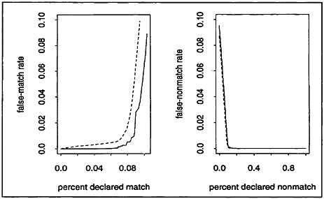
The three-class conditional independence model works for the D88a data, because one of the classes tends to consist of pairs that agree on most comparisons. The medium-sized mixture class tends to agree on variables defining households, but to disagree on personal variables. This class can be called the same household-different person class. The third class tends to disagree on all comparisons. The three-class conditional-independence model also produces good results for the other data sets, except for D90c data. The difference could be caused by the fact that D90c is from a rural area, while the others have a lot of the population in urban settings with better household identifiers.
The search procedure was applied to each of the five data sets. The models selected to start with are given in the second row of Table 3. The number of matches and nonmatches declared matches with estimated false-match rates 005 and 01 are given in lines three and four of Table 3. The number of matches and nonmatches declared nonmatches with estimated false-nonmatch rates 001 and 005 are given in the next two lines. Most models are successfully separating matches and nonmatches. However, in some cases, the rapid rise of estimated false-match rates means few observations can safely be declared matches.
Table 3. —Initial Model Selected for Each Data Set, Along with Matches and Nonmatches Declared Matches and Nonmatches for Two False-Match (FMR) and False-Nonmatch (FNMR) Rates Parentheses enclose (match, nonmatch) counts
|
Data set |
D88a |
D88b |
D90a |
D90b |
D90c |
|
Model |
3C CI |
2C CI-2way |
3C CI |
3C CI |
3C CI-HP |
|
.005 FMR |
(7442,2) |
(0,0) |
(2802,27) |
(2421,12) |
(766,99) |
|
.01 FMR |
(8596,23) |
(24,0) |
(3083,50) |
(2812,25) |
(997,112) |
|
.001 FNMR |
(260, 104587) |
(3455, 49855) |
(124, 33244) |
(69, 34507) |
(32, 36900) |
|
.005 FNMR |
(1021, 105117) |
(3858, 49882) |
(248, 33469) |
(234, 35126) |
(61, 37571) |
|
Total Counts |
(11092, 105213) |
(6878, 49895) |
(3596, 33731) |
(3488, 35307) |
(1261, 37953) |
The models used for D88a, D88b, and D90c were clearly the best candidates among the proposed models for trying to identify matches. In the cases of D90a and D90b, the model with two classes, one with conditional independence between the variables and the other with all two-way interactions, were close competitors to the three-class conditional-independence model. The models chosen for D90a and D90b had estimated error rates that grew slowly until approximately the proportion in the smallest class. The models not chosen had rapidly rising estimated error rates right away.
Pairs were identified to be reviewed by clerks. For the data set D88a, 5000 pairs were reviewed and error rates reestimated. 1000 pairs were reviewed and then the model was refit 5 times. Then 5000 more pairs were reviewed, 1000 at a time. Table 4 contains results for all 5 data sets. For the smaller data sets, fewer observations were reviewed. Note that in Table 4, the reported estimated false-match rates have been reduced. After about ten percent of the pairs are reviewed, most of the matches and nonmatches can be identified with few errors.
Table 4. —Matches and Nonmatches Declared Matches and Nonmatches for Two False-Match (FMR) and False-Nonmatch Rates (FNMR) After Reviewing Some Records and Refitting Models Parentheses enclose (match, nonmatch) counts
|
Data set |
D88a |
D88b |
D90a |
D90b |
D90c |
|
Model |
3C CI |
2C CI-2way |
3C CI |
3C CI |
3C CI-HP |
|
Reviewed |
5000 |
2500 |
2000 |
2000 |
2000 |
|
.001 FMR |
(10764, 0) |
(2703, 1) |
(2620, 10) |
(2562, 8) |
(48, 2) |
|
.005 FMR |
(10917, 27) |
(3105, 8) |
(3447, 26) |
(3347, 17) |
(393,5) |
|
.001 FNMR |
(58, 102728) |
(3339, 49694) |
(104, 33657) |
(76, 35227) |
(40, 37633) |
|
.005 FNMR |
(255, 105212) |
(3448, 49866) |
(316, 33718) |
(206, 35298) |
(121, 37863) |
|
Reviewed |
10000 |
5000 |
4000 |
4000 |
4000 |
|
.001 FMR |
(10916, 13) |
(5057, 1) |
(3439, 1) |
(3341, 3) |
(1019, 5) |
|
.005 FMR |
(10917, 27) |
(6479, 17) |
(3456, 18) |
(3352, 9) |
(1217, 5) |
|
.001 FNMR |
(58, 102728) |
(246, 49857) |
(106, 33688) |
(76, 35236) |
(32, 37994) |
|
.005 FNMR |
(255, 105212) |
(433, 49881) |
(194, 33731) |
(206, 35307) |
(186, 37948) |
|
Total counts |
(11092, 105213) |
(6878, 49895) |
(3596, 33731) |
(3488, 35307) |
(1261, 37953) |
Figure 2 (on the next page) illustrates the impact of the addition of clerk-reviewed data on false-match rate estimates for data set D90c. The method performs better on the other data sets with their models than on D90c.
Conclusion
The development of theory related to applications can be useful for several reasons. The mixture-modeling approach of this paper hopefully can provide some insight into adjustments that are made in applications to make current theory work. Aspects of the new procedure with models parallel actual practice without models. The modeling approach also could improve efficiency by helping clerks identify valuable records to review and then using the additional information through the model to learn more about unclassified observations. More formal model selection procedures and models that allow more complex comparison data will increase the usefulness of the theory.
The goal of this paper has been to demonstrate methods that could be used in new record-linkage situations with big lists where accuracy, automation, and efficiency are needed. The procedure identifies matches and nonmatches, directs clerks in their work, and provides cut-offs and estimates of error rates on five Census data sets.
Acknowledgments
The author wishes to thank William E.Winkler and Donald B.Rubin for their support and guidance in this project. Thanks also to William E.Winkler and Fritz Scheuren for organizing the Record Linkage Workshop.
References
Armstrong, J.B. and Mayda, J.E. ( 1993). Model-Based Estimation of Record Linkage Error Rates, Survey Methodology, 19, 137–147.
Belin, Thomas R. ( 1993). Evaluation of Sources of Variation in Record Linkage Through a Factorial Experiment, Survey Methodology, 19, 13–29.
Belin, Thomas R. and Rubin, Donald B. ( 1995). A Method for Calibrating False-Match Rates in Record Linkage, Journal of the American Statistical Association, 90, 694–707.
Dempster, A.P.; Laird, N.M.; and Rubin, Donald B. ( 1977). Maximum Likelihood from Incomplete Data Via the EM Algorithm, Journal of the Royal Statistical Society, Series B, 39, 1–22, (C/R: 22–37).
Fellegi, Ivan P. and Sumter, Alan B. ( 1969). A Theory for Record Linkage, Journal of the American Statistical Association, 64, 1183–1210.
Goodman, Leo A. ( 1974). Exploratory Latent Structure Analysis Using Both Identifiable and Unidentifiable Models, Biometrika, 61, 215–231.
Haberman, Shelby J. ( 1974). Log-Linear Models for Frequency Tables Derived by Indirect Observation: Maximum Likelihood Equations, The Annals of Statistics, 2, 911–924.
Haberman, Shelby J. ( 1979). Analysis of Qualitative Data, Vol. 2, New York: Academic Press.
Meng, Xiao-Li and Rubin, Donald B. ( 1993). Maximum Likelihood Estimation Via the ECM Algorithm: A General Framework Biometrika, 80, 267–278.
Thibaudeau, Yves. ( 1989). Fitting Log-Linear Models in Computer Matching, Proceedings of the Section on Statistical Computing, American Statistical Association, 283–288.
Thibaudeau, Yves. ( 1993). The Discrimination Power of Dependency Structures in Record Linkage Survey Methodology, 19, 31–38.
Winkler, William E. ( 1988). Using the EM Algorithm for Weight Computation in the Fellegi-Sunter Model of Record Linkage, Proceedings of the Survey Research Methods Section, American Statistical Association, 667–671.
Winkler, William E. ( 1989a). Frequency-Based Matching in the Fellegi-Sunter Model of Record Linkage Proceedings of the Survey Research Methods Section, American Statistical Association, 778- 783.
Winkler, William E. ( 1989b). Near Automatic Weight Computation in the Fellegi-Sunter Model of Record Linkage, Proceedings of the Bureau of the Census Annual Research Conference , 5, 145–155.
Winkler, William E. ( 1989c). Methods for Adjusting for Lack of Independence in an Application of the Fellegi-Sunter Model of Record Linkage, Survey Methodology, 15, 101–117.
Winkler, William E. ( 1990). String Comparator Metrics and Enhanced Decision Rules in the Fellegi-Sunter Model of Record Linkage, Proceedings of the Survey Research Methods Section, American Statistical Association, 354–359.
Winkler, William E. ( 1992), Comparative Analysis of Record Linkage Decision Rules, Proceedings of the Survey Research Methods Section, American Statistical Association , 829–834.
Winkler, William E, ( 1993). Improved Decision Rules in the Fellegi-Sunter Model of Record Linkage Proceedings of the Survey Research Methods Section, American Statistical Association, 274–279.
Winkler, William E. ( 1994). Advanced Methods for Record Linkage, Proceedings of the Survey Research Methods Section, American Statistical Association, 467–472.
Regression Analysis of Data Files that Are Computer Matched—Part I
Fritz Scheuren, Ernst and Young, LLP
William E.Winkler, Bureau of the Census
ABSTRACT
This paper focuses on how to deal with record linkage errors when engaged in regression analysis. Recent work by Rubin and Belin (1991) and by Winkler and Thibaudeau (1991) provides the theory, computational algorithms, and software necessary for estimating matching probabilities. These advances allow us to update the work of Neter, Maynes, and Ramanathan (1965). Adjustment procedures are outlined and some successful simulations are described. Our results are preliminary and intended largely to stimulate further work.
KEY WORDS: Record linkage; Matching error; Regression analysis.
1. INTRODUCTION
Information that resides in two separate computer data bases can be combined for analysis and policy decisions. For instance, an epidemiologist might wish to evaluate the effect of a new cancer treatment by matching information from a collection of medical case studies against a death registry in order to obtain information about the cause and date of death (e.g., Beebe 1985). An economist might wish to evaluate energy policy decisions by matching a data base containing fuel and commodity information for a set of companies against a data base containing the values and types of goods produced by the companies (e.g., Winkler 1985). If unique identifiers, such as verified social security numbers or employer identification numbers, are available, then matching data sources can be straightforward and standard methods of statistical analysis may be applicable directly.
When unique identifiers are not available (e.g., Jabine and Scheuren 1986), then the linkage must be performed using information such as company or individual name, address, age, and other descriptive items. Even when typographical variations and errors are absent, name information such as “Smith” and “Robert” may not be sufficient, by itself, to identify an individual. Furthermore, the use of addresses is often subject to formatting errors because existing parsing or standardization software does not effectively allow comparison of, say, a house number with a house number and a street name with a street name. The addresses of an individual we wish to match may also differ because one is erroneous or because the individual has moved.
Over the last few years, there has been an outpouring of new work on record linkage techniques in North America (e.g., Jaro 1989; and Newcombe, Fair and Lalonde 1992). Some of these results were spurred on by a series of conferences beginning in the mid-1980s (e.g., Kilss and Alvey 1985; Howe and Spasoff 1986; Coombs and Singh 1987; Carpenter and Fair 1989); a further major stimulus in the U.S. has been the effort to study undercoverage in the 1990 Decennial Census (e.g., Winkler and Thibaudeau 1991). The new book by Newcombe (1988) has also had an important role in this ferment. Finally, efforts elsewhere have also been considerable (e.g., Copas and Hilton 1990).
What is surprising about all of this recent work is that the main theoretical underpinnings for computer-oriented matching methods are quite mature. Sound practice dates back at least to the 1950s and the work of Newcombe and his collaborators (e.g., Newcombe et al. 1959). About a decade later, the underlying theory for these basic ideas was firmly established with the papers of Tepping (1968) and, especially, Fellegi and Sunter (1969).
Part of the reason for the continuing interest in record linkage is that the computer revolution has made possible better and better techniques. The proliferation of machine readable files has also widened the range of application. Still another factor has been the need to build bridges between the relatively narrow (even obscure) field of computer matching and the rest of statistics (e.g., Scheuren 1985). Our present paper falls under this last category and is intended to look at what is special about regression analyses with matched data sets.
By and large we will not discuss linkage techniques here. Instead, we will discuss what happens after the link status has been determined. The setting, we will assume, is the typical one where the linker does his or her work separately from the analyst. We will also suppose that the analyst (or user) may want to apply conventional statistical techniques—regression, contingency tables, life tables, etc. — to the linked file. A key question we want to explore then is “What should the linker do to help the analyst?” A
related question is “What should the analyst know about the linkage and how should that information be used?”
In our opinion it is important to conceptualize the linkage and analysis steps as part of a single statistical system and to devise appropriate strategies accordingly. Obviously the quality of the linkage effort may directly impact on any analyses done. Despite this, rarely are we given direct measures of that impact (e.g., Scheuren and Oh 1975). Rubin (1990) has noted the need to make inferential statements that are designed to summarize evidence in the data being analyzed. Rubin's ideas were presented in the connotation of data housekeeping techniques like editing and imputation, where nonresponse can often invalidate standard statistical procedures that are available in existing software packages. We believe Rubin's perspective applies at least with equal force in record linkage work.
Organizationally, our discussion is divided into four sections. First, we provide some background on the linkage setting, because any answers —even partial ones—will depend on the files to be linked and the uses of the matched data. In the next section we discuss our methodological approach, focusing, as already noted, just on regression analysis. A few results are presented in section 4 from some exploratory simulations. These simulations are intended to help the reader weigh our ideas and get a feel for some of the difficulties. A final section consists of preliminary conclusions and ideas for future research. A short appendix containing more on theoretical considerations is also provided.
2. RECORD LINKAGE BACKGROUND
When linking two or more files, an individual record on one file may not be linked with the correct corresponding record on the other file. If a unique identifier for corresponding records on two files is not available—or is subject to inaccuracy—then the matching process is subject to error. If the resultant linked data base contains a substantial proportion of information from pairs of records that have been brought together erroneously or a significant proportion of records that need to be brought together are erroneously left apart, then statistical analyses may be sufficiently compromised that results of standard statistical techniques could be misleading. For the bulk of this paper we will only be treating the situation of how erroneous links affect analyses. The impact of problems caused by erroneous nonlinks (an implicit type of sampling that can yield selection biases) is discussed briefly in the final section.
2.1 Fellegi-Sunter Record Linkage Model
The record linkage process attempts to classify pairs in a product space A × B from two files A and B into M, the set of true links, and U, the set of true nonlinks. Making rigorous concepts introduced by Newcombe (e.g., Newcombe et al. 1959), Fellegi and Sunter (1969) considered ratios of probabilities of the form:
R = Pr(γ ε Γ | M)/Pr(γ ε Γ | U), (2.1)
where γ is an arbitrary agreement pattern in a comparison space Γ. For instance, Γ might consist of eight patterns representing simple agreement or not on surname, first name, and age. Alternatively, each γ ε Γ might additionally account for the relative frequency with which specific surnames, such as Smith or Zabrinsky, occur. The fields that are compared (surname, first name, age) are referred to as matching variables.
The decision rule is given by:
If R > Upper, then designate pair as a link.
If Lower ≤ R ≤ Upper, then designate pair as a possible link and hold for clerical review. (2.2)
If R < Lower, then designate pair as a nonlink.
Fellegi and Sunter (1969) showed that the decision rule is optimal in the sense that for any pair of fixed bounds on R, the middle region is minimized over all decision rules on the same comparison space Γ. The cutoff thresholds Upper and Lower are determined by the error bounds. We call the ratio R or any monotonely increasing transformation of it (such as given by a logarithm) a matching weight or total agreement weight.
In actual applications, the optimality of the decision rule (2.2) is heavily dependent on the accuracy of the estimates of the probabilities given in (2.1). The probabilities in (2.1) are called matching parameters. Estimated parameters are (nearly) optimal if they yield decision rules that perform (nearly) as well as rule (2.2) does when the true parameters are used.
The Fellegi-Sunter approach is basically a direct extension of the classical theory of hypothesis testing to record linkage. To describe the model further, suppose there are two files of size n and m where—without loss of generality— we will assume that n· ≤ m. As part of the linkage process, a comparison might be carried out between all possible n × m pairs of records (one component of the pair coming from each file). A decision is, then, made as to whether or not the members of each comparison-pair represent the same unit or whether there is insufficient evidence to determine link status.
Schematically, it is conventional to look at the n × m pairs arrayed by some measure of the probability that the pair represent records for the same unit. In Figure 1, for example, we have plotted two curves. The curve on the right is a hypothetical distribution of the n true links by the “matching weight” (computed from (2.1) but in natural logarithms). The curve on the left is the remaining of the n × (m − 1) pairs—the true nonlinks—plotted by their matching weights again in logarithms.
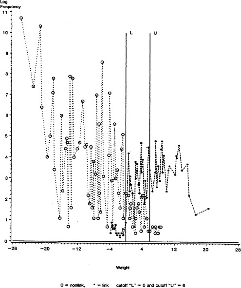
Typically, as Figure 1 indicates, the link and nonlink distributions overlap. At the extremes the overlap is of no consequence in arriving at linkage decisions; however, there is a middle region of potential links, say between “L” and “U”, where it would be hard, based on Figure 1 alone, to distinguish with any degree of accuracy between links and nonlinks.
The Fellegi-Sunter model is valid on any set of pairs we consider. However, for computational convenience, rather than consider all possible pairs in A × B, we might consider only a subset of pairs where the records from both files agree on key or “blocking” information that is thought to be highly accurate. Examples of the logical blocking criteria include items such as a geographical identifier like Postal (e.g., ZIP) code or a surname identifier such as a Soundex or NYSIIS code (see e.g., Newcombe 1988, pp. 182–184). Incidentally, the Fellegi-Sunter Model does not presuppose (as Figure 1 did) that among the n × m pairs there will be n links but rather, if there are no duplicates on A or B, that there will be at most n links.
2.2 Handling Potential Links
Even when a computer matching system uses the Fellegi-Sunter decision rule to designate some pairs as almost certain true links or true nonlinks, it could leave a large subset of pairs that are only potential links. One way to address potentially linked pairs is to clerically review them in an attempt to delineate true links correctly. A way to deal with erroneously nonlinked pairs is to perform additional (again possibly clerical) searches. Both of these approaches are costly, time-consuming, and subject to error.
Not surprisingly, the main focus of record linkage research since the beginning work of Newcombe has been how to reduce the clerical review steps caused by the potential links. Great progress has been made in improving linkage rules through better utilization of information in pairs of records and at estimating error rates via probabilistic models.
Record linkage decision rates have been improved through a variety of methods. To deal with minor typographical errors such as “Smith ” versus “Smoth”, Winkler and Thibaudeau (1991) extended the string comparator metrics introduced by Jaro (1989). Alternatively, Newcombe et al. (1989) developed methods for creating and using partial agreement tables. For certain classes of files, Winkler and Thibaudeau (1991) (see also Winkler 1992; Jaro 1989) developed Expectation-Maximization procedures and ad hoc modelling procedures based on a priori information that automatically yielded the optimal parameters in (2.1) for use in the decision rules (2.2).
Rubin and Belin (1991) introduced a method for estimating error rates, when error rates could not be reliably estimated via conventional methods (Belin 1991, pp. 19–20). Using a model that specified that the curves of weights versus log frequency produced by the matching process could be expressed as a mixture of two curves (links and nonlinks), Rubin and Belin estimated the curves which, in turn, gave estimates of error rates. To apply their method, Rubin and Belin needed a training sample to yield an a priori estimate of the shape of the two curves.
While many linkage problems arise in retrospective, often epidemiological settings, occasionally linkers have been able to designate what information is needed in both data sets to be linked based on known analytic needs. Requiring better matching information, such as was done with the 1990 Census Post-Enumeration Survey (see e.g., Winkler and Thibaudeau 1991), assured that sets of potential links were minimized.
Despite these strides, eventually, the linker and analyst still may have to face a possible clerical review step. Even today, the remaining costs in time, money and hidden residual errors can still be considerable. Are there safe alternatives short of a full review? We believe so and this belief motivates our perspective in section 3, where we examine linkage errors in a regression analysis context. Other approaches, however, might be needed for different analytical frameworks.
3. REGRESSION WITH LINKED DATA
Our discussion of regression will presuppose that the linker has helped the analyst by providing a combined data file consisting of pairs of records—one from each input file—along with the match probability and the link status of each pair. Link, nonlink, and potential links would all be included and identified as such. Keeping likely links and potential links seems an obvious step; keeping likely nonlinks, less so. However, as Newcombe has pointed out, information from likely nonlinks is needed for computing biases. We conjecture that it will suffice to keep no more than two or three pairs of matches from the B file for each record on the A file. The two or three pairs with the highest matching weights would be retained.
In particular, we will assume that the file of linked cases has been augmented so that every record on the smaller of the two files has been paired with, say, the two records on the larger file having the highest matching weights. As n = m, we are keeping 2n of the n × m possible pairs. For each record we keep the linkage indicators and the probabilities associated with the records to which it is paired. Some of these cases will consist of (link, nonlink) combinations or (nonlink, nonlink) combinations. For simplicity's sake, we are not going to deal with settings where more than one true link could occur; hence, (link, link) combinations are by definition ruled out.
As may be quite apparent, such a data structure allows different methods of analysis. For example, we can partition
the file back into three parts—identified links, nonlinks, and potential links. Whatever analysis we are doing could be repeated separately for each group or for subsets of these groups. In the application here, we will use nonlinks to adjust the potential links, and, thereby, gain an additional perspective that could lead to reductions in the Mean Square Error (MSE) over statistics calculated only from the linked data.
For statistical analyses, if we were to use only data arising from pairs of records that we were highly confident were links, then we might be throwing away much additional information from the set of potentially linked pairs, which, as a subset, could contain as many true links as the set of pairs which we designate as links. Additionally, we could seriously bias results because certain subsets of the true links that we might be interested in might reside primarily in the set of potential links. For instance, if we were considering affirmative action and income questions, certain records (such as those associated with lower income individuals) might be more difficult to match using name and address information and, thus, might be heavily concentrated among the set of potential links.
3.1 Motivating Theory
Neter, Maynes, and Ramanathan (1965) recognized that errors introduced during the matching process could adversely affect analyses based on the resultant linked files. To show how the ideas of Neter et al. motivate the ideas in this paper, we provide additional details of their model. Neter et al. assumed that the set of records from one file (1) always could be matched, (2) always had the same probability p of being correctly matched, and (3) had the same probability q of being mismatched to any remaining records in the second file (i.e. p + (N - 1)q = 1 where N is file size). They generalized their basic results by assuming that the sets of pairs from the two files could be partitioned into classes in which (1), (2) and (3) held.
Our approach follows that of Neter et al. because we believe their approach is sensible. We concur with their results showing that if matching errors are moderate then regression coefficients could be severely biased. We do not believe, however, that condition (3)—which was their main means of simplifying computational formulas—will ever hold in practice. If matching is based on unique identifiers such as social security numbers subject to typographical error, it is unlikely that a typographical error will mean that a given record has the same probability of being incorrectly matched to all remaining records in the second file. If matching variables consist of name and address information (which is often subject to substantially greater typographical error), then condition (3) is even more unlikely to hold.
To fix ideas on how our work builds on and generalizes results of Neter et al. we consider a special case. Suppose we are conducting ordinary least squares using a simple regression of the form,
y = a0+ a1x + e. (3.1)
Next, assume mismatches have occurred, so that they variables (from one file) and the x variables (from another file) are not always for the same unit.
Now in this setting, the unadjusted estimator of a1 would be biased; however, under assumptions such as that x and y are independent when a mismatch occurs, it can be shown that, if we know the mismatch rate, h, that an unbiased adjusted estimator can be obtained by simply correcting the ordinary estimator by multiplying it by (1/(1 - h)). Intuitively, the erroneously linked pairs lead to an understatement of the true correlation (positive or negative) between x and y. The adjusted coefficient removes this understatement. With the adjusted slope coefficent ![]() the proper intercept can be obtained from the usual expression
the proper intercept can be obtained from the usual expression ![]() where
where ![]() has been adjusted.
has been adjusted.
Methods for estimating regression standard errors can also be devised in the presence of matching errors. Rather than just continuing to discuss this special case, though, we will look at how the idea of making a multiplicative adjustment can be generalized. Consider
Y = Xß + e, (3.2)
the ordinary univariate regression model, for which error terms all have mean zero and are independent with constant variance s2. If we were working with a data base of size n, Y would be regressed on X in the usual manner. Now, given that each case has two matches, we have 2n pairs altogether. We wish to use (Xi,Yi), but instead use (Xi,Zi). Zi could be Yi, but may take some other value, Yj, due to matching error.
For i = 1, n,
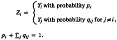
(3.3)
The probability pi may be zero or one. We define hi = 1 - pi and divide the set of pairs into n mutually exclusive classes. The classes are determined by records from one of the files. Each class consists of the independent x-variable Xi, the true value of the dependent y-variable, the values of the y-variables from records in the second file to which the record in the first file containing Xi have been paired, and computer matching probabilities (or weights). Included are links, nonlinks, and potential links. Under an assumption of one-to-one matching, for each i = 1, n, there exists at most one j such that qij> 0. We let f be defined by f(i) = j.
The intuitive idea of our approach (and that of Neter et al.) is that we can, under the model assumptions, express each observed data point pair (X,Z) in terms of the true values (X,Y) and a bias term (X,b). All equations needed for the usual regression techniques can then be obtained. Our computational formulas are much more complicated than those of Neter et al. because their strong assumption (3) made considerable simplification possible in the computational formulas. In particular, under their model assumptions, Neter et al. proved that both the mean and variance of the observed Z-values were necessarily equal the mean and variance of the true Y-values.
Under the model of this paper, we observe (see Appendix) that
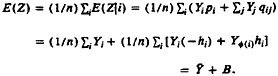
(3.4)
As each Xi, i = 1, n, can be paired with either Yi or Yf(i), the second equality in (3.4) represents 2n points. Similarly, we can represent szy in terms of sxy and a bias term Bxy, and ![]() in terms of
in terms of ![]() and a bias term Byy. We neither assume that the bias terms have expectation zero nor that they are uncorrelated with the observed data.
and a bias term Byy. We neither assume that the bias terms have expectation zero nor that they are uncorrelated with the observed data.
With the different representations, we can adjust the regression coefficients ßzx and their associated standard errors back to the true values ßyx and their associated standardr errors. Our assumption of one-to-one matching (which is not needed for the general theory) is done for computational tractability and to reduce the number of records and amount of information that must be tracked during the matching process.
In implementing the adjustments, we make two crucial assumptions. The first is that, for i = 1, n, we can accurately estimate the true probabilities of a match pi. See Appendix for the method of Rubin and Belin (1991). The second is that, for each i = 1, n, the true value Yi associated with independent variable Xi is the pair with the highest matching weight and the false value Yf(i) is associated with the second highest matching weight. (From the simulations conducted it appears that at least the first of these two assumptions matters greatly when a significant portion of the pairs are potential links.)
3.2 Simulated Application
Using the methods just described, we attempted a simulation with real data. Our basic approach was to take two files for which true linkage statuses were known and re-link them using different matching variables—or really versions of the same variables with different degrees of distortion introduced, making it harder and harder to distinguish a link from a nonlink. This created a setting where there was enough discrimination power for the Rubin-Belin algorithm for estimating probabilities to work, but not so much discriminating power that the overlap area of potential links becomes insignificant.
The basic simulation results were obtained by starting with a pair of files of size 10,000 that had good information for matching and for which true match status was known. To conduct the simulations a range of error was introduced into the matching variables, different amounts of data were used for matching, and greater deviations from optimal matching probabilities were allowed.
Three matching scenarios were considered: (1) good, (2) mediocre, and (3) poor. The good matching scenario consisted of using most of the available procedures that had been developed for matching during the 1990 U.S. Census (e.g., Winkler and Thibaudeau 1991). Matching variables consisted of last name, first name, middle initial, house number, street name, apartment or unit identifier, telephone, age, marital status, relationship to head of household, sex, and race. Matching probabilities used in crucial likelihood ratios needed for the decision rules were chosen close to optimal.
The mediocre matching scenario consisted of using last name, first name, middle initial, two address variations, apartment or unit identifier, and age. Minor typographical errors were introduced independently into one seventh of the last names and one fifth of the first names. Matching probabilities were chosen to deviate from optimal but were still considered to be consistent with those that might be selected by an experienced computer matching expert.
The poor matching scenario consisted of using last name, first name, one address variation, and age. Minor typographical errors were introduced independently into one fifth of the last names and one third of the first names. Moderately severe typographical errors were made in one fourth of the addresses. Matching probabilities were chosen that deviated substantially from optimal. The intent was for them to be selected in a manner that a practitioner might choose after gaining only a little experience.
With the various scenarios, our ability to distinguish between true links and true nonlinks differs significantly. For the good scenario, we see that the scatter for true links and nonlinks is almost completely separated (Figure 2). With the mediocre scheme, the corresponding sets of points overlap moderately (Figure 3); and, with the poor, the overlap is substantial (Figure 4).
We primarily caused the good matching scenario to degenerate to the poor matching error (Figures 2–4) by using less matching information and inducing typographical error in the matching variables. Even if we had kept the same matching variables as in the good matching scenario (Figure 2), we could have caused curve overlap (as in Figure 4) merely by varying the matching
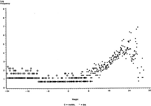
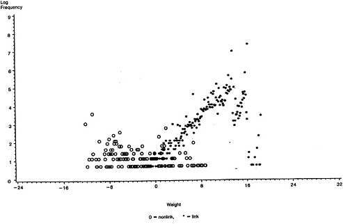
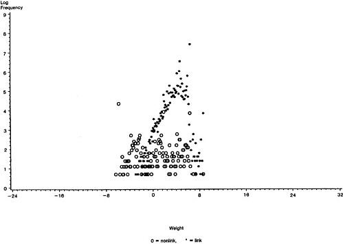
Table 1 Counts of True Links and True Nonlinks and Probabilities of an Erroneous Link in Weight Ranges for Various Matching Cases; Estimated Probabilities via Rubin-Belin Methodology
parameters given by equation (2.1). The poor matching scenario can arise when we do not have suitable name parsing software that allows comparison of corresponding surnames and first names or suitable address parsing software that allows comparison of corresponding house numbers and street names. Lack of proper parsing means that corresponding matching variables associated with many true links will not be properly utilized.
Our ability to estimate the probability of a match varies significantly. In Table 1 we have displayed these probabilities, both true and estimated, by weight classes. For the good and mediocre matching scenarios, estimated probabilities were fairly close to the true values. For the poor scenario, in which most pairs are potential links, deviations are quite substantial.
For each matching scenario, empirical data were created. Each data base contained a computer matching weight, true and estimated matching probabilities, the independent x-variable for the regression, the true dependent y-variable, the observed y-variables in the record having the highest match weight, and the observed y-variable from the record having the second highest matching weight.
The independent x-variables for the regression were constructed using the SAS RANUNI procedure, so as to be uniformly distributed between 1 and 101. For this paper, they were chosen independently of any matching variables. (While we have considered the situation for which regression variables are dependent on one or more matching variables (Winkler and Scheuren 1991), we do not present any such results in this paper.)
Three regression scenarios were then considered. They correspond to progressively lower R2 values: (1) R2 between 0.75 and 0.80; (2) between 0.40 and 0.45; and (3) between 0.20 and 0.22. The dependent variables were generated with independent seeds using the SAS RANNOR procedure. Within each matching scenario (good, mediocre, or poor), all pairing of records obtained by the matching process and, thus, matching error was fixed.
It should be noted that there are two reasons why we generated the (x,y)-data used in the analyses. First, we wanted to be able to control the regression data sufficiently well to determine what the effect of matching error was. This was an important consideration in the very large Monte Carlo simulations reported in Winkler and Scheuren (1991). Second, there existed no available pairs of data files in which highly precise matching information is available and which contain suitable quantitative data.
In performing the simulations for our investigation, some of which are reported here, we created more than 900 data bases, corresponding to a large number of variants of the three basic matching scenarios. Each data base contained three pairs of (x,y)-variables corresponding to the three basic regression scenarios. An examination of these data bases was undertaken to look at some of the matching sensitivity of the regressions and associated adjustments to the sampling procedure. The different data bases determined by different seed numbers are called different samples.
The regression adjustments were made separately for each weight class shown in Table 1, using both the estimated and true probabilities of linkage. In Table 1, weight class 10 refers to pairs having weights between 10 and 11 and weight class -1 refers to pairs having weights between -0 and -1. All pairs having weights 15 and above are combined into class 15 + and all pairs having weights -9 and below are combined into class -10-. While it was possible with the Rubin-Belin results to make individual adjustments for linkage probabilities, we chose to make average adjustments, by each weight class in Table 1. (See Czajka et al. 1992, for discussion of a related decision. Our approach has some of the flavor of the work on propensity scores (e.g., Rosenbaum and Rubin 1983, 1985). Propensity scoring techniques, while proposed for other classes of problems, may have application here as well.
4. SOME HIGHLIGHTS AND LIMITATIONS OF THE SIMULATION RESULTS
Because of space limitations, we will present only a few representative results from the simulations conducted. For more information, including an extensive set of tables, see Winkler and Scheuren (1991).
The two outcome measures from our simulation that we consider are the relative bias and relative standard error. We will only discuss the mediocre matching scenario in detail and only for the case R2 between 0.40 and 0.45. Figures 5–7 shows the relative bias results from a single representative sample. An overall summary, though, for the other scenarios is presented in Table 2. Some limitations on the simulation are also noted at the end of this section.
4.1 Illustrative Results for Mediocre Matching
Rather than use all pairs, we only consider pairs having weights 10 or less. Use of the smaller subset of pairs allows us to examine regression adjustment procedures for weight classes having low to high proportions of true nonlinks. We note that the eliminated pairs (having weight 10 and above) are associated only with true links. Figures 5 and 6 present our results for adjusted and unadjusted regression data, respectively. Results obtained with unadjusted data are based on conventional regression formulas (e.g., Draper and Smith 1981). The weight classes displayed are cumulative beginning with pairs having the highest weight. Weight class w refers to all pairs having weights between w and 10.
We observe the following:
-
The accumulation is by decreasing matching weight (i.e. from classes most likely to consist almost solely of true links to the classes containing increasing higher proportions of true nonlinks). In particular, for weight class w = 8, the first data point shown in Figures 5–7, there were 3 nonlinks and 439 links. By the time, say, we had cumulated the data through weight class w = 5, there were 24 nonlinks; the links, however, had grown to 1,121 —affording us a much larger overall sample size with a corresponding reduction in the regression standard error.
-
Relative biases are provided for the original and adjusted slope coefficient â1 by taking the ratio of the true coefficient (about 2) and the calculated one for each cumulative weight class.
-
Adjusted regression results are shown employing both estimated and true match probabilities. In particular, Figure 5 corresponds to the results obtained using estimated probabilities (all that would ordinarily be available in practice). Figure 7 corresponds to the unrealistic situation for which we knew the true probabilities.
-
Relative root mean square errors (not shown) are obtained by calculating MSEs for each cumulative weight class. For each class, the bias is squared, added to the square of the standard errors, and square roots taken.
Observations on the results we obtained are fairly straightforward and about what we expected. For example, as sample size increased, we found the relative root mean square errors decreasd substantially for the adjusted coefficients. If the regression coefficients were not adjusted,
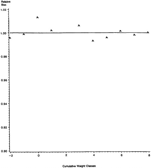
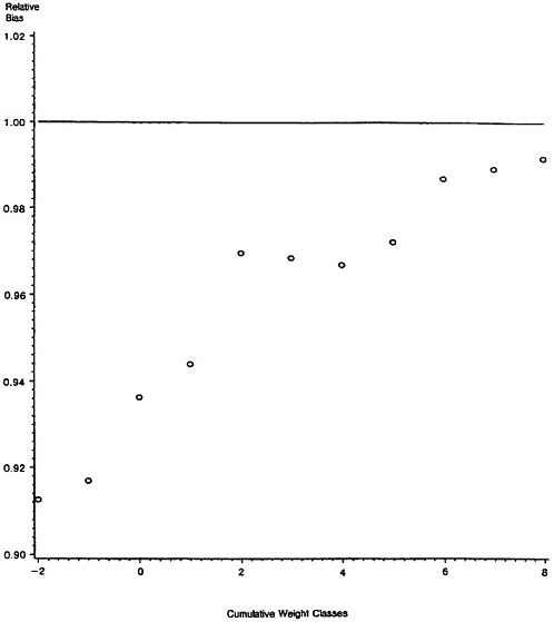
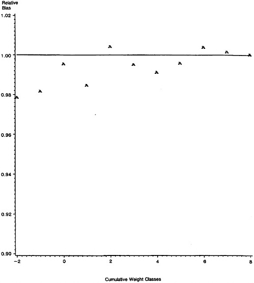
standard errors still decreased as the sample size grew, but at an unacceptably high price in increased bias.
One point of concern is that our ability to accurately estimate matching probabilities critically affects the accuracy of the coefficient estimates. If we can accurately estimate the probabilities (as in this case), then the adjustment procedure works reasonably well; if we cannot (see below), then the adjustment could perform badly.
4.2 Overall Results Summary
Our results varied somewhat for the three different values of R2—being better for larger R2 values. These R2 differences, however, do not change our main conclusions; hence, Table 2 does not address them. Notice that, for the good matching scenario, attempting to adjust does little good and may even cause some minor harm. Certainly it is pointless, in any case, and we only included it in our simulations for the sake of completeness. At the other extreme, even for poor matches, we obtained satisfactory results, but only when using the true probabilities— something not possible in practice.
Table 2 Summary of Adjustment Results for Illustrative Simulations
|
Basis of adjustments |
Matching scenarios |
||
|
Good |
Mediocre |
Poor |
|
|
True probabilities |
Adjustment was not helpful because it was not needed |
Good results like those in Section 4.1 |
Good results like those in Section 4.1 |
|
Estimated probabilities |
Same as above |
Same as above |
Poor results because Rubin-Belin could not estimate the probabilities |
Any statistical estimation procedure will have difficulty with the poor matching scenario because of the extreme overlap of the curves. See Figure 4. We believe the mediocre scenario covers a wide range of typical settings. Nonetheless, the poor matching scenario might arise fairly often too, especially with less experienced linkers. Either new estimation procedures will have to be developed for the poor case or the Rubin-Belin probability estimation procedure —which was not designed for this situation—will have to be enhanced.
4.3 Some Simulation Limitations
The simulation results are subject to a number of limitations. Some of these are of possible major practical significance; others less so. A partial list follows:
-
In conducting simulations for this paper, we assumed that the highest weight pair was a true link and the second highest a true nonlink. This assumption fails because, sometimes, the second highest is the true link and the highest a true nonlink. (We do not have a clear sense of how important this issue might be in practice. It would certainly have to be a factor in poor matching scenarios.)
-
A second limitation of the data sets employed for the simulations is that the truly linked record may not be present at all in the file to which the first file is being matched. (This could be important. In many practical settings, we would expect the “logical blocking criteria” also to cause both pairs used in the adjustment to be false links.)
-
A third limitation of our approach is that no use has been made of conventional regression diagnostic tools. (Depending on the environment, outliers created because of nonlinks could wreak havoc with underlying relationships. In our simulations this did not show up as much of a problem, largely, perhaps, because the X and Y values generated were bounded in a moderately narrow range.)
5. CONCLUSIONS AND FUTURE WORK
The theoretical and related simulation results presented here are obviously somewhat contrived and artificial. A lot more needs to be done, therefore, to validate and generalize our beginning efforts. Nonetheless, some recommendations for current practice stand out, as well as areas for future research. We will cover first a few of the topics that intrigued us as worthy of more study to improve the adjustment of potential links. Second, some remarks are made about the related problem of what to do with the (remaining) nonlinks. Finally, the section ends with some summary ideas and a revisitation of our perspective concerning the unity of the tasks that linkers and analysts do.
5.1 Improvements in Linkage Adjustment
An obvious question is whether our adjustment procedures could borrow ideas from general methods for errors-in-variables (e.g., Johnston 1972). We have not explored this, but there may be some payoffs.
Of more interest to us are techniques that grow out of conventional regression diagnostics. A blend of these with our approach has a lot of appeal. Remember we are making adjustments, weight class by weight class. Suppose we looked ahead of time at the residual scatter in a particular weight class, where the residuals were calculated around the regression obtained from the cumulative weight classes above the class in question. Outliers, say, could then be identified and might be treated as nonlinks rather than potential links.
We intend to explore this possibility with simulated data that is heavier-tailed than what was used here. Also we will explore consciously varying the length of the weight classes and the minimum number of cases in each class. We have an uneasy feeling that the number of cases in each class may have been too small in places. (See Table 1.) On the other hand, we did not use the fact that the weight classes were of equal length nor did we study what would have happened had they been of differing lengths.
One final point, as noted already: we believe our approach has much in common with propensity scoring, but we did not explicitly appeal to that more general theory for aid and this could be something worth doing. For example, propensity scoring ideas may be especially helpful in the case where the regression variables and the linkage variables are dependent. (See Winkler and Scheuren (1991) for a report on the limited simulations undertaken and the additional difficulties encountered.)
5.2 Handling Erroneous Nonlinks
In the use of record linkage methods the general problem of selection bias arises because of erroneous nonlinks. There are a number of ways to handle this. For example, the links could be adjusted by the analyst for lack of representativeness, using the approaches familiar to those who adjust for unit or, conceivably, item nonresponse (e.g., Scheuren et al. 1981).
The present approach for handling potential links could help reduce the size of the erroneous nonlink problem but, generally, would not eliminate it. To be specific, suppose we had a linkage setting where, for resource reasons, it was infeasible to follow up on the potential links. Many practitioners, might simply drop the potential links, thereby, increasing the number of erroneous nonlinks. (For instance, in ascertaining which of a cohort's members is alive or dead, a third possibility—unascertained—is often used.)
Our approach to the potential links would have implicitly adjusted for that portion of the erroneous nonlinks which were potentially linkable (with a followup step, say). Other erroneous nonlinks would generally remain and another adjustment for them might still be an issue to consider.
Often we can be faced with linkage settings where the files being linked have subgroups with matching information of varying quality, resulting in differing rates of erroneous links and nonlinks. In principle, we could employ the techniques in this paper to each subgroup separately. How to handle very small subgroups is an open problem and the effect on estimated differences between subgroups, even when both are of modest size, while seemingly straightforward, deserves study.
5.3 Concluding Comments
At the start of this paper we asked two “key” questions. Now that we are concluding, it might make sense to reconsider these questions and try, in summary fashion, to give some answers.
-
“What should the linker do to help the analyst?” If possible, the linker should play a role in designing the datasets to be matched, so that the identifying information on both is of high quality. Powerful algorithms exist now in several places to do an excellent job of linkage (e.g., at Statistics Canada or the U.S. Bureau of the Census, to name two). Linkers should resist the temptation to design and develop their own software. In most cases, modifying or simply using existing software is highly recommended (Scheuren 1985). Obviously, for the analyst 's sake, the linker needs to provide as much linkage information as possible on the files matched so that the analyst can make informed choices in his or her work. In the present paper we have proposed that the links, nonlinks, and potential links be provided to the analyst—not just links. We strongly recommend this, even if a clerical review step has been undertaken. We do not necessarily recommend the particular choices we made about the file structure, at least not without further study. We would argue, though, that our choices are serviceable.
-
“What should the analyst know about the linkage and how should this be used?” The analyst needs to have information like link, nonlink, and potential link status, along with linkage probabilities, if available. Many settings could arise where simply doing the data analysis steps separately by link status will reveal a great deal about the sensitivity of one's results. The present paper provides some initial ideas about how this use might be approached in a regression context. There also appears to be some improvements possible using the adjustments carried out here, particularly for the mediocre matching scenario. How general these improvements are remains to be seen. Even so, we are relatively pleased with our results and look forward to doing more. Indeed, there are direct connections to be made between our approach to the regression problem and other standard techniques, like contingency table loglinear models.
Clearly, we have not developed complete, general answers to the questions we raised. We hope, though, that this paper will at least stimulate interest on the part of others that could lead us all to better practice.
ACKNOWLEDGMENTS AND DISCLAIMERS
The authors would like to thank Yahia Ahmed and Mary Batcher for their help in preparing this paper and two referees for detailed and discerning comments. Fruitful discussions were held with Tom Belin. Wendy Alvey also provided considerable editorial assistance.
The usual disclaimers are appropriate here: in particular, this paper reflects the views of the authors and not necessarily those of their respective agencies. Problems, like a lack of clarity in our thinking or in our exposition, are entirely the authors' responsibility.
APPENDIX
The appendix is divided into four sections. The first provides details on how matching error affects regression models for the simple univariate case. The approach most closely resembles the approach introduced by Neter et al. (1965) and provides motivation for the generalizations presented in appendix sections two and three. Computational formulas are considerably more complicated than those presented by Neter et al. because we use a more realistic model of the matching process. In the second section, we extend the univariate model to the case for which all independent variables arise from one file, while the dependent variable comes from the other, and, in the third, we extend the second case to that in which some independent variables come from one file and some come from another. The fourth section summarizes methods of Rubin and Belin (1991) (see also Belin 1991) for estimating the probability of a link.
A.1. Univariate Regression Model
In this section we address the simplest regression situation in which we match two files and consider a set of numeric pairs in which the independent variable is taken from a record in one file and the dependent variable is taken from the corresponding matched record from the other file.
Let Y = Xβ + ε be the ordinary univariate regression model for which error terms are independent with expectation zero and constant variance σ2. If we were working with a single data base, Y would be regressed on X in the usual manner. For i = 1, . . . , n, we wish to use (Xi,Yi) but we will use (Xi,Zi), where Zi is usually Yi but it may take some other value Yj due to matching error.
That is, for i = 1, . . . , n,
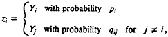
where pi + Σj≠1qij = 1.
The probability pi may be zero or one. We define hi = 1 − pi. As in Neter et al. (1965), we divide the set of pairs into n mutually exclusive classes. Each class consists of exactly one (Xi,Zi) and, thus, there are n classes. The intuitive idea of our procedure is that we basically adjust Zi, in each (Xi,Zi) for the bias induced by the matching process. The accuracy of the adjustment is heavily dependent on the accuracy of the estimates of the matching probabilities in our model.
To simplify the computational formulas in the explanation, we assume one-to-one matching; that is, for each i = 1, . . . , n, there exists at most one j such that qij > 0. We let φ be defined by φ(i) = j. Our model still applies if we do not assume one-to-one matching.
As intermediate steps in estimating regression coefficients and their standard errors, we need to find μz≡ E(Z), ![]() and σzx. As in Neter et al. (1965),
and σzx. As in Neter et al. (1965),
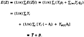
(A.1.1)
The first and second equalities are by definition and the third is by addition and subtraction. The third inequality is the first time we apply the one-to-one matching assumption. The last term on the right hand side of the equality is the bias which we denote by B. Note that the overall bias B is the statistical average (expectation) of the individual biases [Yi(−hi) + Y(i)hi] for i = 1, . . . , n. Similarly, we have
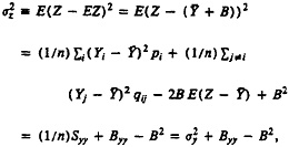
(A.1.2)
where ![]()
![]() and
and ![]()
(A.1.3)
where ![]()
![]() and syx = (1/n)Syx. The term Byy is the bias for the second moments and the term Byx is the bias for the cross-product of Y and X. Formulas (A.1.1), (A.1.2), and (A.1.3), respectively, correspond to formulas (A.1), (A.2), and (A.3) in Neter et al. The formulas necessarily differ in detail because we use a more general model of the matching process.
and syx = (1/n)Syx. The term Byy is the bias for the second moments and the term Byx is the bias for the cross-product of Y and X. Formulas (A.1.1), (A.1.2), and (A.1.3), respectively, correspond to formulas (A.1), (A.2), and (A.3) in Neter et al. The formulas necessarily differ in detail because we use a more general model of the matching process.
The regression coefficients are related by
(A.1.4)
To get an estimate of the variance of ßyx, we first derive an estimate s2 for the variance s2 in the usual manner.
(A.1.5)
Using (A.1.2) and (A.1.3) allows us to express s2 in terms of the observable quantities ![]() and szx and the bias terms Byy, Byx, and B that are computable under our assumptions. The estimated variance of ßyx is then computed by the usual formula (e.g., Draper and Smith 1981, 18–20)
and szx and the bias terms Byy, Byx, and B that are computable under our assumptions. The estimated variance of ßyx is then computed by the usual formula (e.g., Draper and Smith 1981, 18–20)
We observe that the first equality in (A.1.5) involves the usual regression assumption that the error terms are independent with identical variance.
In the numeric examples of this paper we assumed that the true independent value Xi associated with each Yi was from the record with the highest matching weight and the false independent value was taken from the record with the second highest matching weight. This assumption is plausible because we have only addressed simple regression in this paper and because the second highest matching weight was typically much lower than the highest. Thus, it is much more natural to assume that the record with the second highest matching weight is false. In our empirical examples we use straightforward adjustments and make simplistic assumptions that work well because they are consistent with the data and the matching process. In more complicated regression situations or with other models such as loglinear we will likely have to make additional modelling assumptions. The additional assumptions can be likened to the manner in which simple models for nonresponse require additional assumptions as the models progress from ignorable to nonignorable (see Rubin 1987).
In this section, we chose to adjust independent x-values and leave dependents-values as fixed in order to achieve consistency with the reasoning of Neter et al. We could have just as easily adjusted dependent y-values leaving x-values as fixed.
A.2. Multiple Regression with Independent Variables from One File and Dependent Variables from the Other File
At this point we pass to the usual matrix notation (e.g., Graybill 1976). Our basic model is
Y = Xß + e,
where Y is a n × 1 array, X is a n × p array, ß is a p × 1 array, and e is a n × 1 array.
Analogous to the reasoning we used in (A.1.1), we can represent
Z = Y + B, (A.2.1)
where Z, Y, and B are n × 1 arrays having terms that correspond, for i = 1, n, via
zi= yi+piyi+ hiyf(i).
Because we observe Z and X only, we consider the equation
Z = XC + e. (A.2.2)
We obtain an estimate ![]() by regressing on the observed data in the usual manner. We wish to adjust the estimate
by regressing on the observed data in the usual manner. We wish to adjust the estimate ![]() to an estimate
to an estimate ![]() of ß in a manner analogous to (A.1.1).
of ß in a manner analogous to (A.1.1).
Using (A.2.1) and (A.2.2) we obtain
(A.2.3)
The first term on the left hand side of (A.2.3) is the usual estimate ![]() . The second term on the left hand side of (A.2.3) is our bias adjustment. XT is the transpose of X.
. The second term on the left hand side of (A.2.3) is our bias adjustment. XT is the transpose of X.
The usual formula (Graybill 1976, p. 176) allows estimation of the variance s2 associated with the i.i.d. error components of e,
(A.2.4)
Via (A.2.1) can ![]() be represented in terms of the observable Z and X in a manner similar to (A.1.2) and (A.1.3). As
be represented in terms of the observable Z and X in a manner similar to (A.1.2) and (A.1.3). As
YTY = ZTZ - BTZ - ZTB - BTB, (A.2.5)
we can obtain the remaining portion of the right hand side of (A.2.4) that allows estimation of s2.
Via the usual formula (e.g., Graybill 1976, p. 276), the covariance of ![]() is
is
(A.2.6)
which we can estimate.
A.3. Multiple Regression with Independent Variables from Both Files
When some of the independent variables come from the same file as Y we must adjust them in a manner similar to the way in which we adjust Y in equations. (A.1.1) and (A.2.1). Then data array X can be written in the form
Xd= X + D, (A.3.1)
where D is the array of bias adjustments taking those terms of X arising from the same file as Y back to their true values that are represented in Xd. Using (A.2.1) and (A.2.2), we obtain
Y + B = (Xd− D)C. (A.3.2)
With algebra (A.3.2) becomes
(A.3.3)
If D is zero (i.e., all independent x-values arise from a single file), then (A.3.3) agrees with (A.2.3). The first term on the left hand side of (A.2.3) is the estimate of ![]() . The estimate
. The estimate ![]() is obtained analogously to the way (A.2.3), (A.2.4)
is obtained analogously to the way (A.2.3), (A.2.4) ![]() and (A.2.5) were used. The covariance of
and (A.2.5) were used. The covariance of ![]() follows from (A.2.6).
follows from (A.2.6).
To estimate the probabilty of a true link within any weight range, Rubin and Belin (1991) consider the set of pairs that are produced by the computer matching program and that are ranked by decreasing weight. They assume that the probability of a true link is a montone function of the weight; that is, the higher the weight, the higher the probability of a true link. They assume that the distribution of the observed weights is a mixture of the distributions for true links and true nonlinks.
Their estimation procedure is:
-
Model each of the two components of the mixture as normal with unknown mean and variance after separate power transformations.
-
Estimate the power of the two transformations from a training sample.
-
Taking the two transformations as known, fit a normal mixture model to the current weight data to obtain maximum likelihood estimates (and standard errors).
-
Use the parameters from the fitted model to obtain point estimates of the false-link rate as a function of cutoff level and obtain standard errors for the false-link rate using the delta-method approximation.
While the Rubin-Belin method requires a training sample, the training sample is primarily used to get the shape of the curves. That is, if the power transformation is given by
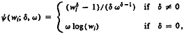
where ω is the geometric mean of the weights wi, i = 1, . . . , n, then ω and δ can be estimated for the two curves. For the examples of this paper and a large class of other matching situations (Winkler and Thibaudeau 1991), the Rubin-Belin estimation procedure works well. In some other situations a different method (Winkler 1992) that uses more information than the Rubin-Belin method and does not require a training sample yields accurate estimates, while software (see e.g., Belin 1991) based on the Rubin-Belin method fails to converge even if new calibration data are obtained. Because the calibration data for the good and mediocre scenarios of this paper are appropriate, the Rubin-Belin method provides better estimates than the method of Winkler.
REFERENCES
BEEBE, G.W. ( 1985). Why are epidemiologists interested in matching algorithms? In Record Linkage Techniques—1985. U.S. Internal Revenue Service.
BELIN, T. ( 1991). Using Mixture Models to Calibrate Error Rates in Record Linkage Procedures, with Application to Computer Matching for Census Undercount Estimation . Harvard Ph.D. thesis.
CARPENTER, M., and FAIR, M.E. (Editors) ( 1989). Proceedings of the Record Linkage Sessions and Workshop, Canadian Epidemiological Research Conference, Statistics Canada.
COOMBS, J.W., and SINGH, M.P. (Editors) ( 1987). Proceedings: Symposium on Statistical Uses of Administrative Data, Statistics Canada.
COPAS, J.B., and HILTON, F.J. ( 1990). Record linkage: Statistical models for matching computer records. Journal of the Royal Statistical Society A, 153, 287–320.
CZJAKA, J.L., HIRABAYASHI, S.M., LITTLE, R.J.A., and RUBIN, D.B. ( 1992). Evaluation of a new procedure for estimating income and tax aggregrates from advance data. Journal of Business and Economic Statistics, 10, 117–131.
DRAPER, N.R., and SMITH, H. ( 1981). Applied Regression Analysis, 2nd Edition. New York: J.Wiley.
FELLEGI, I.P., and SUNTER, A. ( 1969). A theory of record linkage. Journal of the of the American Statistical Association, 64, 1183–1210.
GRAYBILL, F.A. ( 1976). Theory and Application of the Linear Model. Belmont, CA: Wadsworth.
HOWE, G., and SPASOFF, R.A. (Editors) ( 1986). Proceedings of the Workshop on Computerized Record Linkage in Health Research . Toronto, Ontario, Canada: University of Toronto Press.
JABINE, T.B., and SCHEUREN, F.J. ( 1986). Record linkages for statistical purposes: methodological issues. Journal of Official Statistics, 2, 255–277.
JARO, M.A. ( 1989). Advances in record-linkage methodology as applied to matching the 1985 Census of Tampa, Florida. Journal of the American Statistical Association, 84, 414–420.
JOHNSTON, J. ( 1972). Econometric Methods, 2nd Edition. New York: McGraw-Hill.
KILSS, B., and ALVEY, W. (Editors) ( 1985). Record Linkage Techniques—1985. U.S. Internal Revenue Service, Publication 1299, 2–86.
NEWCOMBE, H.B. ( 1988). Handbook of Record Linkage: Methods for Health and Statistical Studies, Administration and Business . Oxford: Oxford University Press.
NEWCOMBE, H.B., FAIR, M.E., and LALONDE, P. ( 1992). The use of names for linking personal records. Journal of the Americal Statistical Association, 87, 1193–1208.
NEWCOMBE, H.B., KENNEDY, J.M., AXFORD, S.J., and JAMES, A.P. ( 1959). Automatic linkage of vital records. Science, 130, 954–959.
NETER, J., MAYNES, E.S., and RAMANATHAN, R. ( 1965). The effect of mismatching on the measurement of response errors. Journal of the American Statistical Association, 60, 1005–1027.
ROSENBAUM, P., and RUBIN, D. ( 1983). The central role of the propensity score in observational studies for causal effects. Biometrika, 70, 41–55.
ROSENBAUM, P., and RUBIN, D. ( 1985). Constructing a control group using multivariate matched sampling methods that incorporate the propensity score. The American Statistician, 39, 33–38.
RUBIN, D.B. ( 1987). Multiple Imputation for Nonresponse in Surveys. New York: J.Wiley.
RUBIN, D.B. ( 1990). Discussion (of Imputation Session). Proceedings of the 1990 Annual Research Conference, U.S. Bureau of the Census, 676–678.
RUBIN, D., and BELIN, T. ( 1991). Recent developments in calibrating error rates for computer matching Proceedingsof the 1991 Annual Research Conference, U.S. Bureau of the Census, 657–668.
SCHEUREN, F. ( 1985). Methodologic issues in linkage of multiple data bases. Record Linkage Techniques—1985. U.S. Internal Revenue Service.
SCHEUREN, F., and OH, H.L. ( 1975). Fiddling Around with Nonmatches and Mismatches. Proceedings of the Social Statistics Section, American Statistical Association, 627–633.
SCHEUREN, F., OH, H.L., VOGEL, L., and YUSKAVAGE, R. ( 1981). Methods of Estimation for the 1973 Exact Match Study. Studies from Interagency Data Linkages, U.S. Department of Health and Human Services, Social Security Administration, Publication 13–11750.
TEPPING, B.J. ( 1968). A model for optimum linkage of records. Journal of the American Statistical Association, 63, 1321–1332.
WINKLER, W.E. ( 1985). Exact matching list of businesses: blocking, subfield identification, and information theory. In Record Linkage Techniques—1985, (Eds. B.Kilss and W.Alvey). U.S. Internal Revenue Service, Publication 1299, 2–86.
WINKLER, W.E. ( 1992). Comparative analysis of record linkage decision rules. Proceedings of the Section on Survey Research Methods, American Statistical Association, to appear.
WINKLER, W.E., and SCHEUREN, F. ( 1991). How Computer Matching Error Effects Regression Analysis: Exploratory and Confirmatory Analysis. U.S. Bureau of the Census, Statistical Research Division Technical Report.
WINKLER, W.E., and THIBAUDEAU, Y. ( 1991). An Application of the Fellegi-Sunter Model of Record Linkage to the 1990 U.S. Census. U.S. Bureau of the Census, Statistical Research Division Technical Report.
Regression Analysis of Data Files that are Computer Matched—Part II*
Fritz Scheuren, Ernst and Young, LLP
William E.Winkler, Bureau of the Census
Abstract
Many policy decisions are best made when there is supporting statistical evidence based on analyses of appropriate microdata. Sometimes all the needed data exist but reside in multiple files for which common identifiers (e.g., SIN's, EIN's, or SSN's) are unavailable. This paper demonstrates a methodology for analyzing two such files: when there is common nonunique information subject to significant error and when each source file contains noncommon quantitative data that can be connected with appropriate models. Such a situation might arise with files of businesses only having difficult-to-use name and address information in common, one file with the energy products consumed by the companies, and the other file containing the types and amounts of goods they produce. Another situation might arise with files on individuals in which one file has earnings data, another information about health-related expenses, and a third information about receipts of supplemental payments. The goal of the methodology presented is to produce valid statistical analyses; appropriate microdata files may or may not be produced.
Introduction
Application Setting
To model the energy economy properly, an economist might need company-specific microdata on the fuel and feedstocks used by companies that are only available from Agency A and corresponding microdata on the goods produced for companies that is only available from Agency B. To model the health of individuals in society, a demographer or health science policy worker might need individual-specific information on those receiving social benefits from Agencies B1, B2, and B3, corresponding income information from Agency I, and information on health services from Agencies H1 and H2. Such modeling is possible if analysts have access to the microdata and if unique, common identifiers are available (e.g., Oh and Scheuren, 1975; Jabine and Scheuren, 1986). If the only common identifiers are error-prone or nonunique or both, then probabilistic matching techniques (e.g., Newcombe et al., 1959, Fellegi and Sunter, 1969) are needed.
Relation To Earlier Work
In earlier work (Scheuren and Winkler, 1993), we provided theory showing that elementary regression analyses could be accurately adjusted for matching error, employing knowledge of the quality of the matching. In that work, we relied heavily on an error-rate estimation procedure of Belin and Rubin (1995). In later research (Winkler and Scheuren, 1995, 1996), we showed that we could make further improvements by using noncommon quantitative data from the two files to improve matching and adjust statistical analyses for matching error. The main requirement — even in heretofore seemingly impossible situations—was that there exist a reasonable model for the relationships
|
* |
Reprinted with permission. To appear in Survey Methodology (1997), 23, 2. |
among the noncommon quantitative data. In the empirical example of this paper, we use data for which a very small subset of pairs can be accurately matched using name and address information only and for which the noncommon quantitative data is at least moderately correlated. In other situations, researchers might have a small microdata set that accurately represents relationships of noncommon data across a set of large administrative files or they might just have a reasonable guess at what the relationships among the noncommon data are. We are not sure, but conjecture that, with a reasonable starting point, the methods discussed here will succeed often enough to be of general value.
Basic Approach
The intuitive underpinnings of our methods are based on now well-known probabilistic record linkage (RL) and edit/imputation (EI) technologies. The ideas of modern RL were introduced by Newcombe (Newcombe et al., 1959) and mathematically formalized by Fellegi and Sunter (1969). Recent methods are described in Winkler (1994, 1995). EI has traditionally been used to clean up erroneous data in files. The most pertinent methods are based on the EI model of Fellegi and Holt (1976).
To adjust a statistical analysis for matching error, we employ a four-step recursive approach that is very powerful. We begin with an enhanced RL approach (e.g., Winkler, 1994; Belin and Rubin, 1995) to delineate a subset of pairs of records in which the matching error rate is estimated to be very low. We perform a regression analysis, RA, on the low-error-rate linked records and partially adjust the regression model on the remainder of the pairs by applying previous methods (Scheuren and Winkler, 1993). Then, we refine the EI model using traditional outlier-detection methods to edit and impute outliers in the remainder of the linked pairs. Another regression analysis (RA) is done and this time the results are fed back into the linkage step so that the RL step can be improved (and so on). The cycle continues until the analytic results desired cease to change. Schematically, these analytic linking methods take the form

Structure of What Follows
Beginning with this introduction, the paper is divided into five sections. In the second section, we undertake a short review of Edit/Imputation (EI) and Record Linkage (RL) methods. Our purpose is not to describe them in detail but simply to set the stage for the present application. Because Regression Analysis (RA) is so well known, our treatment of it is covered only in the particular simulated application (Section 3). The intent of these simulations is to use matching scenarios that are more difficult than what most linkers typically encounter. Simultaneously, we employ quantitative data that is both easy to understand but hard to use in matching. In the fourth section, we present results. The final section consists of some conclusions and areas for future study.
EI and RL Methods Reviewed
Edit/Imputation
Methods of editing microdata have traditionally dealt with logical inconsistencies in data bases. Software consisted of if-then-else rules that were data-base-specific and very difficult to maintain or modify, so as to keep current. Imputation methods were part of the set of if-then-else rules and could yield revised records that still failed edits. In a major theoretical advance that broke with prior statistical methods, Fellegi and Holt (1976)
introduced operations-research-based methods that both provided a means of checking the logical consistency of an edit system and assured that an edit-failing record could always be updated with imputed values, so that the revised record satisfies all edits. An additional advantage of Fellegi-Holt systems is that their edit methods tie directly with current methods of imputing microdata (e.g., Little and Rubin 1987).
Although we will only consider continuous data in this paper, EI techniques also hold for discrete data and combinations of discrete and continuous data. In any event, suppose we have continuous data. In this case a collection of edits might consist of rules for each record of the form
c1X < Y < c2X.
In words,
Y can be expected to be greater than c1X and less than c2X; hence, if Y less than c1X and greater than c2X, then the data record should be reviewed (with resource and other practical considerations determining the actual bounds used).
Here Y may be total wages, X the number of employees, and c1 and c2 constants such that c1< c2. When an (X, Y) pair associated with a record fails an edit, we may replace, say, Y with an estimate (or prediction).
Record Linkage
A record linkage process attempts to classify pairs in a product space A × B from two files A and B into M, the set of true links, and U, the set of true nonlinks. Making rigorous concepts introduced by Newcombe (e.g., Newcombe et al., 1959; Newcombe et al, 1992), Fellegi and Sunter (1969) considered ratios R of probabilities of the form
R = Pr ((γεΓ|M)/Pr((γεΓ|U)
where γ is an arbitrary agreement pattern in a comparison space Γ. For instance, Γ might consist of eight patterns representing simple agreement or not on surname, first name, and age. Alternatively, each γεΓ might additionally account for the relative frequency with which specific surnames, such as Scheuren or Winkler, occur. The fields compared (surname, first name, age) are called matching variables. The decision rule is given by
If R > Upper , then designate pair as a link.
If Lower ≤ R ≤ Upper, then designate pair as a possible link and hold for clerical review.
If R < Lower, then designate pair as a nonlink.
Fellegi and Sunter (1969) showed that this decision rule is optimal in the sense that for any pair of fixed bounds on R, the middle region is minimized over all decision rules on the same comparison space Γ. The cutoff thresholds, Upper and Lower, are determined by the error bounds. We call the ratio R or any monotonely increasing transformation of it (typically a logarithm) a matching weight or total agreement weight.
With the availability of inexpensive computing power, there has been an outpouring of new work on record linkage techniques (e.g., Jaro, 1989, Newcombe, Fair, Lalonde, 1992, Winkler, 1994, 1995). The new computer-intensive methods reduce, or even sometimes eliminate, the need for clerical review when name, address, and other information used in matching is of reasonable quality. The proceedings from a recently concluded international conference on record linkage showcases these ideas and might be the best single reference (Alvey and Jamerson, 1997).
Simulation Setting
Matching Scenarios
For our simulations, we considered a scenario in which matches are virtually indistinguishable from nonmatches. In our earlier work (Scheuren and Winkler, 1993), we considered three matching scenarios in which matches are more easily distinguished from nonmatches than in the scenario of the present paper.
In both papers, the basic idea is to generate data having known distributional properties, adjoin the data to two files that would be matched, and then to evaluate the effect of increasing amounts of matching error on analyses. Because the methods of this paper work better than what we did earlier, we only consider a matching scenario that we label “Second Poor,” because it is more difficult than the poor (most difficult) scenario we considered previously.
We started here with two population files (sizes 12,000 and 15,000), each having good matching information and for which true match status was known. The settings were examined: high, medium and low—depending on the extent to which the smaller file had cases also included in the larger file. In the high file inclusion situation, about 10,000 cases are on both files for an file inclusion or intersection rate on the smaller or base file of about 83%. In the medium file intersection situation, we took a sample of one file so that the intersection of the two files being matched was approximately 25%. In the low file intersection situation, we took samples of both files so that the intersection of the files being matched was approximately 5%. The number of intersecting cases, obviously, bounds the number of true matches that can be found.
We then generated quantitative data with known distributional properties and adjoined the data to the files. These variations are described below and displayed in Figure 1 where we show the poor scenario (labeled “first poor”) of our previous 1993 paper and the “second poor” scenario used in this paper. In the figure, the match weight, the logarithm of R, is plotted on the horizontal axis with the frequency, also expressed in logs, plotted on the vertical axis. Matches (or true links) appear as asterisks (*), while nonmatches (or true nonlinks) appear as small circles (o).
“First Poor” Scenario (Figure 1a)
The first poor matching scenario consisted of using last name, first name, one address variation, and age. Minor typographical errors were introduced independently into one fifth of the last names and one third of the first names in one of the files. Moderately severe typographical errors were made independently in one fourth of the addresses of the same file. Matching probabilities were chosen that deviated substantially from optimal. The intent was for the links to be made in a manner that a practitioner might choose after gaining only a little experience. The situation is analogous to that of using administrative lists of individuals where information used in matching is of poor quality. The true mismatch rate here was 10.1%.
Figure 1a. 1st Poor Matching Scenario
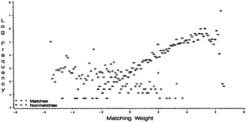
“Second Poor” Scenario (Figure 1b)
The second poor matching scenario consisted of using last name, first name, and one address variation. Minor typographical errors were introduced independently into one third of the last names and one third of the first names in one of the files. Severe typographical errors were made in one fourth of the addresses in the same file. Matching probabilities were chosen that deviated substantially from optimal. The intent was to represent situations that often occur with lists of businesses in which the linker has little control over the quality of the lists. Name information—a key identifying characteristic —is often very difficult to compare effectively with business lists. The true mismatch rate was 14.6%.
Figure 1b. 2nd Poor Matching Scenario
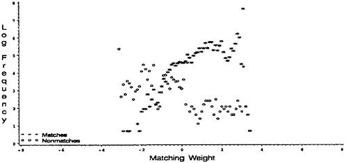
Summary of Matching Scenarios
Clearly, depending on the scenario, our ability to distinguish between true links and true nonlinks differs significantly. With the first poor scenario, the overlap, shown visually between the log-frequency-versus-weight curves is substantial (Figure 1a); and, with the second poor scheme, the overlap of the log-frequency-versus-weight curves is almost total (Figure 1b). In the earlier work, we showed that our theoretical adjustment procedure worked well using the known true match rates in our data sets. For situations where the curves of true links and true nonlinks were reasonably well separated, we accurately estimated error rates via a procedure of Belin and Rubin (1995) and our procedure could be used in practice. In the poor matching scenario of that paper (first poor scenario of this paper), the Belin-Rubin procedure was unable to provide accurate estimates of error rates but our theoretical adjustment procedure still worked well. This indicated that we either had to find an enhancement to the Belin-Rubin procedures or to develop methods that used more of the available data. (That conclusion, incidentally, from our earlier work led, after some false starts, to the present approach.)
Quantitative Scenarios
Having specified the above linkage situations, we used SAS to generate ordinary least squares data under the model Y = 6 X + e,. The X values were chosen to be uniformly distributed between 1 and 101. The error terms, are normal and homoscedastic with variances 13000, 36000, and 125000, respectively. The resulting regressions of Y on X have R2 values in the true matched population of 70%, 47%, and 20%, respectively. Matching with quantitative data is difficult because, for each record in one file, there are hundreds of records having quantitative values that are close to the record that is a true match. To make modeling and analysis even more difficult in the high file overlap scenario, we used all false matches and only 5% of the true matches; in the medium file overlap scenario, we used all false matches and only 25% of true matches. (Note: Here to heighten the visual effect, we have introduced another random sampling step, so the reader can “see” better in the figures the effect of bad matching. This sample depends on the match status of the case and is confined only to those cases that were matched, whether correctly or falsely.)
A crucial practical assumption for the work of this paper is that analysts are able to produce a reasonable model (guesstimate) for the relationships between the noncommon quantitative items. For the initial modeling in the empirical example of this paper, we use the subset of pairs for which matching weight is high and the error-rate is low. Thus, the number of false matches in the subset is kept to a minimum. Although neither the procedure of Belin and Rubin (1995) nor an alternative procedure of Winkler (1994), that requires an ad hoc intervention, could be used to estimate error rates, we believe it is possible for an experienced matcher to pick out a low-error-rate set of pairs even in the second poor scenario.
Simulation Results
Most of this Section is devoted to presenting graphs and results of the overall process for the second poor scenario, where the R2 value is moderate, and the intersection between the two files is high. These results best illustrate the procedures of this paper. At the end of the Section (in subsection 4.8), we summarize results over all R2 situations and all overlaps. To make the modeling more difficult and show the power of the analytic linking methods, we use all false matches and a random sample of only 5% of the true matches. We only consider pairs having matching weight above a lower bound that we determine based on analytic considerations and experience. For the pairs of our analysis, the restriction causes the number of false matches to significantly exceed the number of true matches. (Again, this is done to heighten the visual effect of matching failures and to make the problem even more difficult.)
To illustrate the data situation and the modeling approach, we provide triples of plots. The first plot in the triple shows the true data situation as if each record in one file was linked with its true corresponding record in the other file. The quantitative data pairs correspond to the truth. In the second plot, we show the observed data. A high proportion of the pairs is in error because they correspond to false matches. To get to the third plot in the triple, we model using a small number of pairs (approximately 100) and then replace outliers with pairs in which the observed Y-value is replaced with a predicted Y-value.
Initial True Regression Relationship
In Figure 2a, the actual true regression relationship and related scatterplot are shown, for one of our simulations, as they would appear if there were no matching errors. In this figure and the remaining ones, the true regression line is always given for reference. Finally, the true population slope or beta coefficient (at 5.85) and the R2 value (at 43%) are provided for the data (sample of pairs) being displayed.
Figure 2a. 2nd Poor Scenario, 1st Pass All False & 5% True Matches, True Data, HighOverlap 1104 Points, beta=5.85, R–square=0.43
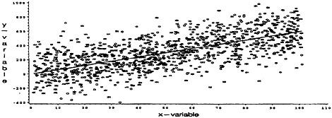
Regression after Initial RL ⇒ RA Step
In Figure 2b, we are looking at the regression on the actual observed links—not what should have happened in a perfect world but what did happen in a very imperfect one. Unsurprisingly, we see only a weak regression relationship between Y and X. The observed slope or beta coefficient differs greatly from its true value (2.47 v. 5.85). The fit measure is similarly affected—falling to 7% from 43%.
Figure 2b. 2nd Poor Scenario, 1st Pass All False & 5% True Matches, Observed Data, HighOverlap 1104 Points, beta=2.47, R–square=0.07
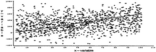
Regression After First Combined RL ⇒ RA ⇒ EI ⇒ RA Step
Figure 2c completes our display of the first cycle of the iterative process we are employing. Here we have edited the data in the plot displayed as follows. First, using just the 99 cases with a match weight of 3.00 or larger, an attempt was made to improve the poor results given in figure 2b. Using this provisional fit, predicted values were obtained for all the matched cases; then outliers with residuals of 460 or more were removed and the regression refit on the remaining pairs. This new equation, used in figure 2c, was essentially Y = 4.78X + ε, with a variance of 40000. Using our earlier approach (Scheuren and Winkler, 1993), a further adjustment was made in the estimated beta coefficient from 4.78 to 5.4. If a pair of matched records yielded an outlier, then predicted values (not shown) using the equation Y = 5.4X were imputed. If a pair does not yield an outlier, then the observed value was used as the predicted value.
Figure 2c. 2nd Poor Scenario, 1st Pass All False & 5% True Matches, Outlier—Adjusted Data 1104 Points, beta= 4.78, R–square=0.40

Second True Reference Regression
Figure 3a displays a scatterplot of X and Y as they would appear if they could be true matches based on a second RL step. Note here that we have a somewhat different set of linked pairs this time from earlier, because we have used the regression results to help in the linkage. In particular, the second RL step employed the predicted Y values as determined above; hence it had more information on which to base a linkage. This meant that a different group of linked records was available after the second RL step. Since a considerably better link was obtained, there
Figure 3a. 2nd Poor Scenario, 2nd Pass All False & 5% True Matches, True Data, High Overlap 650 Points, beta= 5.91, R–square=0.48
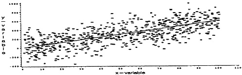
were fewer false matches; hence our sample of all false matches and 5% of the true matches dropped from 1104 in Figures 2a thru 2c to 650 for Figures 3a thru 3c. In this second iteration, the true slope or beta coefficient and the R2 values remained, though, virtually identical for the estimated slope (5.85 v. 5.91) and fit (43% v. 48%).
Regression After Second RL ⇒ RA Step
In Figure 3b, we see a considerable improvement in the relationship between Y and X using the actual observed links after the second RL step. The estimated slope has risen from 2.47 initially to 4.75 here. Still too small but much improved. The fit has been similarly affected, rising from 7% to 33%.
Figure 3b. 2nd Poor Scenario, 2nd Pass All False & 5% True Matches, Observed Data, High Overlap 650 Points, beta=4.75, R–square=0.33
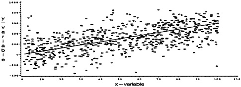
Regression After Second Combined RL⇒RA⇒EI⇒RA Step
Figure 3c completes the display of the second cycle of our iterative process. Here we have edited the data as follows. Using the fit (from subsection 4.5), another set of predicted values was obtained for all the matched cases (as in subsection 4.3). This new equation was essentially Y = 5.26X + ε, with a variance of about 35000. If a pair of matched records yields an outlier, then predicted values using the equation Y = 5.3X were imputed. If a pair does not yield an outlier, then the observed value was used as the predicted value.
Figure 3c. 2nd Poor Scenario, 2nd Pass All False & 5% True Matches, Outlier—Adjusted Data 650 Points, beta=5.26, R–square=0.47
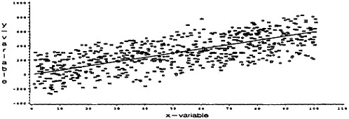
Additional Iterations
While we did not show it in this paper, we did iterate through a third matching pass. The beta coefficient, after adjustment, did not change much. We do not conclude from this that asymptotic unbiasedness exists; rather that the method, as it has evolved so far, has a positive benefit and that this benefit may be quickly reached.
Further Results
Our further results are of two kinds. We looked first at what happened in the medium R2 scenario (i.e., R2 equal to 47) for the medium- and low- file intersection situations. We further looked at the cases when R2 was higher (at 70) or lower (at 20). For the medium R2 scenario and low intersection case the matching was somewhat easier. This occurs because there were significantly fewer false-match candidates and we could more easily separate true matches from false matches. For the high R2 scenarios, the modeling and matching were also more straightforward than there were for the medium R2 scenario. Hence, there were no new issues there either.
On the other hand, for the low R2 scenario, no matter what degree of file intersection existed, we were unable to distinguish true matches from false matches, even with the improved methods we are using. The reason for this, we believe, is that there are many outliers associated with the true matches. We can no longer assume, therefore, that a moderately higher percentage of the outliers in the regression model are due to false matches. In fact, with each true match that is associated with an outlier Y-value, there may be many false matches that have Y-values that are closer to the predicted Y-value than the true match.
Comments and Future Study
Overall Summary
In this paper, we have looked at a very restricted analysis setting: a simple regression of one quantitative dependent variable from one file matched to a single quantitative independent variable from another file. This standard analysis was, however, approached in a very nonstandard setting. The matching scenarios, in fact; were quite challenging. Indeed, just a few years ago, we might have said that the “second poor” matching scenario appeared hopeless.
On the other hand, as discussed below, there are many loose ends. Hence, the demonstration given here can be considered, quite rightly in our view, as a limited accomplishment. But make no mistake about it, we are doing something entirely new. In past record linkage applications, there was a clear separation between the identifying data and the analysis data. Here, we have used a regression analysis to improve the linkage and the improved linkage to improve the analysis and so on.
Earlier, in our 1993 paper, we advocated that there be a unified approach between the linkage and the analysis. At that point, though, we were only ready to propose that the linkage probabilities be used in the analysis to correct for the failures to complete the matching step satisfactorily. This paper is the first to propose a completely unified methodology and to demonstrate how it might be carried out.
Planned Application
We expect that the first applications of our new methods will be with large business data bases. In such situations, noncommon quantitative data are often moderately or highly correlated and the quantitative variables
(both predicted and observed) can have great distinguishing power for linkage, especially when combined with name information and geographic information, such as a postal (e.g., ZIP) code.
A second observation is also worth making about our results. The work done here points strongly to the need to improve some of the now routine practices for protecting public use files from reidentification. In fact, it turns out that in some settings—even after quantitative data have been confidentiality protected (by conventional methods) and without any directly identifying variables present—the methods in this paper can be successful in reidentifying a substantial fraction of records thought to be reasonably secure from this risk (as predicted in Scheuren, 1995). For examples, see Winkler, 1997.
Expected Extensions
What happens when our results are generalized to the multiple regression case? We are working on this now and results are starting to emerge which have given us insight into where further research is required. We speculate that the degree of underlying association R2 will continue to be the dominant element in whether a usable analysis is possible.
There is also the case of multivariate regression. This problem is harder and will be more of a challenge. Simple multivariate extensions of the univariate comparison of Y values in this paper have not worked as well as we would like. For this setting, perhaps, variants and extensions of Little and Rubin (1987, Chapters 6 and 8) will prove to be a good starting point.
“Limited Accomplishment”
Until now an analysis based on the second poor scenario would not have been even remotely sensible. For this reason alone we should be happy with our results. A closer examination, though, shows a number of places where the approach demonstrated is weaker than it needs to be or simply unfinished. For those who want theorems proven, this may be a particularly strong sentiment. For example, a convergence proof is among the important loose ends to be dealt with, even in the simple regression setting. A practical demonstration of our approach with more than two matched files also is necessary, albeit this appears to be more straightforward.
Guiding Practice
We have no ready advise for those who may attempt what we have done. Our own experience, at this point, is insufficient for us to offer ideas on how to guide practice, except the usual extra caution that goes with any new application. Maybe, after our own efforts and those of others have matured, we can offer more.
References
Alvey, W. and Jamerson, B. (eds.) ( 1997), Record Linkage Techniques —1997 (Proceedings of An International Record Linkage Workshop and Exposition, March 20–21, 1997, in Arlington VA).
Belin, T. R,, and Rubin, D.B. ( 1995). A Method for Calibrating False-Match Rates in Record Linkage, Journal of the American Statistical Association, 90, 694–707.
Fellegi, I. and Holt, T. ( 1976). A Systematic Approach to Automatic Edit and Imputation, Journal of the of the American Statistical Association, 71, 17–35.
Fellegi, I. and Sunter, A. ( 1969). A Theory of Record Linkage, Journal of the of the American Statistical Association, 64, 1183–1210.
Jabine, T.B. and Scheuren, F. ( 1986). Record Linkages for Statistical Purposes: Methodological Issues, Journal of Official Statistics, 2, 255–277.
Jaro, M.A. ( 1989). Advances in Record-Linkage Methodology as Applied to Matching the 1985 Census of Tampa, Florida, Journal of the American Statistical Association, 89, 414–420.
Little, R.J. A. and Rubin, D.B. ( 1987). Statistical Analysis with Missing Data, J.Wiley: New York.
Newcombe, H.B.; Kennedy, J.M.; Axford, S.J.; and James, A.P. ( 1959). Automatic Linkage of Vital Records, Science, 130, 954–959.
Newcombe, H.; Fair, M.; and Lalonde, P. ( 1992). The Use of Names for Linking Personal Records, Journal of the American Statistical Association, 87, 1193–1208.
Oh, H.L. and Scheuren, F. ( 1975). Fiddling Around with Mismatches and Nonmatches, Proceedings of the Section on Social Statistics, American Statistical Association.
Scheuren, F. and Winkler, W.E. ( 1993). Regression Analysis of Data Files that are Computer Matched, Survey Methodology, 19, 39–58.
Scheuren, F. ( 1995). Review of Private Lives and Public Policies, Journal of the American Statistical Association, 90.
Scheuren, F. and Winkler, W.E. ( 1996). Recursive Merging and Analysis of Administrative Lists and Data, Proceedings of the Section of Government Statistics, American Statistical Association, 123–128.
Winkler, W.E. ( 1994). Advanced Methods of Record Linkage, Proceedings of the Section of Survey Research Methods, American Statistical Association, 467–472.
Winkler, W.E. ( 1995). Matching and Record Linkage, in B.G.Cox et al. (ed.), Business Survey Methods, New York: J.Wiley, 355–384.
Winkler, W.E. and Scheuren, F. ( 1995). Linking Data to Create Information, Proceedings of Statistics Canada Symposium, 95.
Winkler, W.E. and Scheuren, F. ( 1996). Recursive Analysis of Linked Data Files, Proceedings of the 1996 Census Bureau.
Winkler, W.E. ( 1997), Producing Public-Use Microdata That are Analytically Valid and Confidential Paper presented at the 1997 Joint Statistical Meetings in Anaheim


