
6
INTERPOLATION, NONLINEAR SMOOTHING, FILTERING, AND PREDICTION
The topics of smoothing and filtering, commonly referred to as “data assimilation” in the oceanographic and meteorological literature, have attracted a great deal of attention of late. This emphasis on the combination of statistical with dynamical methods, relatively new to oceanography, arises as a natural consequence of the increasing sophistication of models, the rapid increase in available computing power, and the availability of new extensive data sets.
The most extensive of these newly available and soon to be available data sets are remotely sensed from space. Active and passive instruments operating in the microwave, infrared, and visible portions of the electromagnetic spectrum provide spatial and temporal coverage of the ocean unavailable from any other source, but present new challenges in interpretation. In particular, problems of filling in temporal and spatial gaps in the data, interpolating satellite data sets to model grids, and selecting a limited number of points from very large data sets in order to formulate tractable computational problems must be considered.
INTERPOLATION OF SATELLITE DATA SETS
Characteristics of Satellite Data
Different satellite instruments pose different problems, depending on spatial and temporal coverage, effects of clouds and rain cells, and viewing geometries. Characteristically, satellite data are sampled very rapidly (on the order of seconds or minutes). Data are acquired as areal averages along the satellite ground track, as in the case of the altimeter, which samples a region 10 km wide, or as areal averages of patches 5 to 50 km in diameter in swaths 1000 km wide in the cross-track direction, as in the case of the scatterometer or AVHRR. Spatially overlapping samples are taken on the order of 10 days later in the case of line samples, or on the order of 1 day later in the case of swaths.
The satellite altimeter, as indicated in Table 2.1 of Chapter 2, takes measurements roughly every 7 km along the track. Employing active microwave radar, the altimeter functions in both day and night hours, in the presence of clouds, or in clear weather. Two sets of satellite tracks, corresponding to ascending and descending orbits (i.e., orbits that cross the equator moving northward or southward, respectively) form a nonrectangular network that is oriented at an angle with respect to the parallels and meridians of latitude and longitude. The angles change as functions of the distance from the equator, as do the separations between adjacent tracks in the same direction (Figure 6.1). The irregular space-time sampling inherent in satellite measurements over an ocean basin raises important questions about aliasing and the range in wavenumber-frequency space that can be resolved
by the data. The problem is very difficult, and only a few attempts have thus far been made to address the issue (Wunsch, 1989; Schlax and Chelton, 1992).
Satellite instruments, such as AVHRR, that work in the visible and infrared range of the electromagnetic spectrum provide ocean observations only in the absence of clouds. Hence, maps based on these observations have gaps. One way of achieving full coverage of a specific ocean area is by creating composite images that combine data from different time periods (cf., NRC, 1992a). However, since the fields (for example, sea surface temperature) are time dependent, the composite images represent only some average picture of sea surface temperature distribution for the period covered. Therefore, it is important to know how this picture and its statistical properties are connected with the statistical properties of cloud fields, and how representative the composite image is with respect to the ensemble average of the temperature field (see, e.g., Chelton and Schlax, 1991).
Mapping Satellite Data: Motivation and Methods
For most applications, satellite data must be represented on a regular grid. The most common method of mapping satellite observations onto a geographic grid is by interpolating the data from nearby points at the satellite measurement locations. Given the complicated statistical geometry of oceanographic fields (see Chapter 2), such gridding may lead to considerable distortion. Therefore, it is important to study effects of intermittent and rare events, as well as effects of statistical anisotropy and inhomogeneity of oceanographic fields, on the gridding process.
Each interpolated value is typically computed from the 10 to 1000 closest data points, selected from the millions of points typically found in satellite data sets. Common non-trivial methods of interpolating include natural or smoothing spline fits, successive corrections, statistical interpolation, and fitting analytical basis functions such as spherical harmonics. In all cases the interpolated values are linear functions of some judiciously chosen subset of the data.
Applications of natural splines and smoothing splines to interpolate irregularly spaced data are as common in oceanography as they are in most other fields of science and engineering. The methods have been well documented in the literature (e.g., Press et al., 1986; Silverman, 1985).
Successive corrections (Bratseth, 1986; Tripoli and Krishnamurti, 1975) is an iterative scheme, with one iteration per spatial and temporal scale starting with the larger ones. The interpolating weights are a function only of the scale and an associated quantity, the search radius (e.g., Gaussian of given width arbitrarily set to zero for distances greater than the search radius). This scheme is computationally very fast and adapts reasonably well to irregular data distributions, but does not usually provide a formal error estimate of the interpolated field, although it is straightforward to add one. Somewhat related is an iterative scheme that solves the differential equation for minimum curvature (Swain, 1976) of the interpolated surfaces with predetermined stiffness parameter, akin to cubic splines; however, the extension to three-dimensional data is not commonly available.
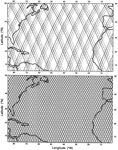
FIGURE 6.1 Example pattern of satellite ground tracks for the Geosat altimeter (see Douglas and Cheney, 1990, and Vol. 95, Nos. C3 and C10 of J.Geophys. Res.) with a 17-day exact repeat orbit configuration. Upper panel shows the ground tracks traced out during days 1 to 3 (solid lines), days 4 to 6 (dashed lines), and days 7 to 9 (dotted lines) of each 17-day repeat cycle. Note the eastward shift of a coarse-resolution ground track pattern at 3-day intervals. Lower panel shows the complete grid of ground tracks sampled during each 17-day cycle. SOURCE: Courtesy of Dudley Chelton, Oregon State University.
Statistical interpolation (Gandin, 1965; Alaka and Elvander, 1972; Bretherton et al., 1976), also referred to as optimal interpolation and most generally referred to as objective mapping (despite the fact that all of the techniques described here are objective), consists of least-squares fitting between interpolated and data fields. It assumes that estimates are known and available of the covariance matrix of the data with errors, and of the field to be interpolated. This is formally identical to ordinary least squares regression, in which the value of the interpolated field at a given point is assumed to be a linear function of the data at nearby points, and the moment and cross-product matrices are determined by assumptions about the spatial and temporal covariance of the underlying field. The formulas for the coefficients are derived simply by taking the expected values of the matrices in the ordinary least squares regression formula. Because matrix inversions are required for each set of estimates, the computational requirement is typically an order of magnitude larger than with the successive correction scheme. Formal error estimates are always given. Kriging (Journel and Huijbregts, 1978; NRC, 1992a) is a similar method in which the structure function rather than covariance is used to describe the data and desired field, with somewhat better adaptability to inhomogeneous statistics. The equivalence of objective analysis and spline interpolation was presented by McIntosh (1990).
Projecting the data on a space spanned by a convenient set of nonlocal basis functions is simple and well known, but there is no obvious choice of an efficient set of basis functions. The spherical harmonics commonly used for this purpose in meteorology do not form an efficient basis over the oceanic domain alone, requiring high-degree terms just to adapt to the domain. Recent efforts to define an equivalent set only over the oceans (Hwang, 1991) appear to have been successful.
The disadvantage of using L2 norm minimizations is their relatively high computer resource requirement. An insidious consequence of this high resource demand is that in order to limit the problem to a size manageable with available computer resources, some researchers use too few data values or too small a region to achieve proper isolation of the length scales of signal and error. The disadvantage of schemes with fixed weights is clear: they are unable to adapt to data of varying accuracy, even though they do a decent job at adapting to inhomogeneous data distributions. The practical disadvantage for both objective mapping and successive corrections is that spatially inhomogeneous scales and anisotropy are not easily treated, and require breaking up the problem into several regional ones. This can lead to inconsistencies or other undesirable problems along the boundaries of adjacent regions. In the case of basis functions, most natural choices prove to be very inefficient in representing small-scale features; e.g., many higher-degree terms may be required to define a narrow jet such as the Gulf Stream.
DATA ASSIMILATION: USE OF DYNAMICAL MODELS FOR SMOOTHING AND FILTERING
As discussed in Chapter 1, it is not possible even with satellite data sets to provide complete initial and boundary conditions for the models in use today. This is partly due to physical considerations, such as the unknown details of air-sea exchanges, but the greatest
limitation on modeling studies today remains the sparsity of data, especially subsurface data that are inaccessible via satellites. It is therefore necessary to extract all available information from the data while, simultaneously, understanding the limitations on the applicability of any given data set.
Most data assimilation work to date has been based on least-squares formulations and the resulting linearized mathematical formalism. This can be justified rigorously for linear systems under fairly general conditions, assuming the initial error distributions are Gaussian. Within their realm of applicability, linearized methods have been quite successful. The ocean modeling community has a fair amount of experience with filtering and smoothing of linear models. The major remaining issues involve validation of statistical error models. These issues are most fruitfully considered in the contexts of specific problems. A review of data assimilation in oceanography can be found in Ghil and Malanotte-Rizzoli (1991). For a general overview, see NRC (1991a).
The use of ocean circulation models in smoothing and filtering of observational data has a relatively short history. Still, there have been a number of successful attempts (e.g., Thacker and Long, 1988; Gaspar and Wunsch, 1989; Miller and Cane, 1989). A recent excellent study is that of Fukumori et al. (1992). There has been, however, little systematic study of nonlinear smoothing and filtering in the context of ocean modeling. The ocean modeling literature naturally overlaps with the numerical weather prediction literature on this subject, and the two fields share a common interest in qualitative results, but systematic studies are few, and those that exist are elementary.
Direct approaches to applying statistically based data assimilation methods to nonlinear problems have so far been based on generalizations of linear methods. Variational methods used to date (e.g., Tziperman and Thacker, 1989; Bennett and Thorburn, 1992; Miller et al., 1992; Moore, 1991) have been derived from quadratic cost functions; i.e., the optimized solution is the one that minimizes some combination of covariances. This presupposes the notion that minimizing quadratic moments is the right thing to do in this context, even though the underlying distribution may not be unimodal. As one might expect, these methods work well in problems in which the nonlinearity is weak, or at least does not result in qualitatively nonlinear behavior such as bifurcation or chaos. Model studies have been performed on the Lorenz equations (Gauthier, 1992; Miller et al., 1992), which, for the most part, used covariance statistics and linearized methods. (An application in which third and fourth moments were calculated explicitly was presented by Miller et al. (1993), but it is unlikely that this method has any wider applicability). Gauthier (1992) and Miller et al. (1993) discuss in detail the pitfalls in filtering and smoothing of highly nonlinear problems. In those cases, the implementation of variational methods results in extreme computational difficulty.
The solution to the nonlinear filtering problem for randomly perturbed dynamical systems is well understood theoretically (see Rozovskii, 1990). It can be reduced to a solution of the so-called Zakai equation, a second-order stochastic parabolic equation. It describes the evolution of the non-normalized density of the state vector conditioned upon observations. Smoothing and prediction are technically based on the Zakai equation and the so-called backward filtering equation (see Rozovskii, 1990). In the last decade substantial progress has also been made in numerical studies of the Zakai equation (see, e.g.,
Florchinger and LeGland, 1990). However, this theoretically perfect approach has some practical limitations. In particular, the dimension of the spatial variable for the Zakai equation is equal to the dimension of the state vector. This is clearly impractical for modern dynamical ocean models that have thousands, if not hundreds of thousands, of state variables.
It appears that the most promising approach to this problem is development of hierarchical methods that would involve Kalman-type filtering where possible and refinement of the first-level coarse filtering by application of intrinsically nonlinear procedures when necessary. These require further research on numerical approximation for Zakai-type stochastic partial differential equations, including development of stochastic versions for multigrid methods, wavelets, and so on.
While true nonlinear filtering will not find direct application to practical ocean models in the near future, guidance from solutions of simplified problems can be expected. Further, there may be approximations to the Zakai equation in terms of parametric representations to solutions that are more versatile than those derived from methods explored earlier.
Overall, it appears that numerical methods for stochastic systems are developing into an exciting area of science that is of importance to oceanographic data assimilation.
INVERSE METHODS
Some oceanographers consider that, in some larger sense, all of physical oceanography can be described in terms of an inverse problem: given data, describe the ocean from which the data were sampled. Obviously direct inversion of the sampling process is impossible, but the smoothing process is occasionally viewed as some generalized inverse of the sampling process, with the laws of ocean physics used as constraints (see, e.g., Wunsch, 1978, 1988; Bennett, 1992).
It has become common in oceanography and dynamic meteorology to solve the smoothing problem by assuming that the system in question is governed exactly by a given dynamical model. Since the output of many dynamical models is determined uniquely by the initial condition, the problem becomes one of finding the initial conditions that result in model output that is closest to the observed data in some sense; the metric most commonly used has been least squares. These problems are usually solved by a conjugate gradient method, and the gradient of the mean square data error with respect to the initial values can be calculated conveniently by solving an adjoint equation. For that reason, this procedure is often referred to as the adjoint method. (see, e.g., Tziperman and Thacker, 1989). This is formally an inverse problem, i.e.: when given the outputs in the form of the data, find the inputs in the form of the initial conditions.
There are many significant problems in physical oceanography that bear specific resemblance to what is formally called inverse theory in other fields such as geophysics. These include estimation of empirical parameters (e.g., diffusion coefficients) and the design of sampling arrays to yield the most detailed picture of the property being sampled. Problems such as these, along with others that fall within the strict category of smoothing and filtering, are described in detail in the volume by Bennett (1992).
PROSPECTIVE DIRECTIONS FOR RESEARCH
There are many opportunities for statistical and probabilistic research regarding interpolation, smoothing, filtering, and prediction associated with oceanographic data. The following are some of the contexts that present challenges:
-
Filtering and smoothing for the systems in which the dynamics are given by discontinuous functions of the state variables;
-
Parameter estimation for randomly perturbed equations of physical oceanography;
-
Alternative numerical and analytical approaches to the least-squares approach for nonlinear systems;
-
Hierarchical methods of filtering, prediction, and smoothing;
-
Spectral methods for nonlinear filtering (separation of observations and parameters);
-
Multigrid and decomposition of the domain for Zakai’s equation; and
-
Application of inverse methods for (a) data interpolation, (b) estimation of empirical and/or phenomenological parameters, and (c) design of sampling arrays.
In particular, progress in answering the following questions would certainly be beneficial:
-
What is the best way to solve the smoothing problem in cases where the dynamics are given by discontinuous functions of the state variable? Such examples are common in models of the upper ocean in which convection takes place. Possibly the best ocean model known, that of Bryan (1969) and Cox (1984), deals with this problem by assuming that the heat conductivity becomes infinite if the temperature at a given level is colder than it is below that level. The result is instantaneous mixing of the water, to simulate the rapid time scale of convection in nature. This can be viewed as an inequality constraint on the state vector; i.e., some regions of state space are deemed to be inadmissible solutions of the problem. Such problems are treated in the control theory literature (see, e.g., Bryson and Ho, 1975), but the engineering methods are not conveniently applicable to high-dimensional state spaces.
-
If the least-squares approach is inadequate for highly nonlinear systems, what would be better?
-
What is the best way to apply solutions of the nonlinear filtering problem to more complex systems? Might it be possible to implement the extended Kalman filter for a
-
relatively simple system and use the resulting covariance statistics in a suboptimal data assimilation scheme for a more detailed model? In general, how might the hierarchical approach suggested in the section above on data assimilation (also cf., NRC 1992a) be implemented?
-
When should one statistical method be applied as opposed to another? What diagnostics are there to help make decisions on suitable methods? Answers to such questions could be compiled in a handbook on statistical analysis of oceanographic and atmospheric data, could include such things as definitions and methods of statistical parameter estimation, and could discuss such questions as, e.g., What do these parameters convey?
-
What statistical methods can be used for cross-validating data that take inherent averaging errors into account, and that provide estimates of their magnitude? With the advent of remote sensing, data comparison (Chapter 7) is not limited merely to measurements and model verification, but involves cross-validation of different sensors or assimilation of data into models for quality assessment (see NRC, 1991a). In such analyses, each data set contains errors that are inherent to the averaging process. As Dickey (1991, p. 410) has noted:
One of the major challenges from both the atmospheric and ocean sciences is to merge and integrate in situ and remotely sensed interdisciplinary data sets which have differing spatial and temporal resolution and encompass differing scale ranges…. Interdisciplinary data assimilation models, which require subgrid parametrizations based on higher resolution data, will need to utilize these data sets for applications such as predicting trends in the global climate.


