
Appendix
Cocaine Markets and Supply-Control Activities
This appendix presents a formal model of supply and demand for cocaine and uses the model to investigate how supply-control activities may affect market outcomes. The model described here seeks to express in a relatively simple fashion many of the essential features of the RAND model, while abstracting from much of that model's complexity. In one important respect, the model described here explores territory outside the domain of the RAND model: It permits the average cost function that determines industry supply to be upward sloping rather than downward sloping. With this elaboration, it is possible to investigate the sensitivity of the RAND findings to plausible variations in the shape of the average cost curve.
Basic Elements Of The Model
The basic elements of the model include a demand function specifying the quantity of cocaine demanded at any given price, a cost function specifying the cost of producing any given quantity of cocaine, and a market-clearing mechanism explaining how consumers and producers interact to determine the equilibrium quantity and price of cocaine. As in the RAND model, supply-control activities are measured through the magnitude of seizures of cocaine production.
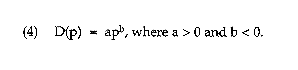
On the demand side, let p denote the price variable and let D(p) be the quantity demanded as a function of price. On the supply side, let X denote the magnitude of cocaine seizures and let q denote the cocaine
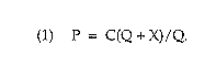
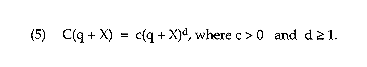
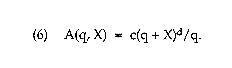
production that escapes seizure. Thus, q + X is total industry production. Let C(q + X) denote the total cost of producing this amount of cocaine. Let Q be the equilibrium 'quantity of cocaine that escapes seizure and left P be the equilibrium price.
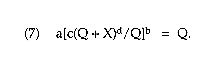
As in the RAND study, assume that equilibrium price equals the average cost of cocaine production, measured as total cost divided by the amount of cocaine that escapes seizure. Thus,
The equilibrium quantity that escapes seizure equals the quantity demanded at the equilibrium price. Thus,

Combining these two conditions yields

Solving this equation for Q yields the equilibrium consumption of cocaine as a function of the magnitude X of seizures. Given specifications for the demand function D(•) and the cost function C(•), one may use (3) to study how cocaine consumption responds to variations in seizures.
Specification Of The Demand And Cost Functions
As in the RAND study, assume that demand has the constant-elasticity form
In a departure from the RAND study, assume that the cost function has the power-function form
The average cost per unit of production that escapes seizure is then
The RAND study essentially assumes the special case of (5) and (6) in which d = 1, implying constant marginal costs and downward sloping average costs. Here we entertain the possibility that d > 1, implying that
marginal cost increases with production. Inspection of the derivative of the average cost function (6) with respect to q shows that the average cost function is downward sloping when q < X/(d - 1) but upward sloping when q > X/(d - 1).
Analysis Of Market Equilibrium
Given equations (4) and (6), the equilibrium condition (3) becomes
The goal is to determine how the equilibrium quantity Q varies with magnitude X of seizures. However, the easiest way to study the equilibrium condition is to solve (7) for X as a function of Q. This yields
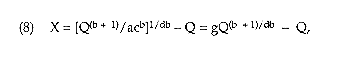
where g = (acb)-1/db.
If the demand elasticity b is in the range - 1 < b < 0, the right side of equation (8) is a decreasing function of Q. In particular, the right side of (8) decreases from ∞ to -∞ as Q rises from 0 to ∞. This implies that there is a unique equilibrium, with the equilibrium consumption Q being a decreasing function of seizures X. If b < -1, there may be multiple equilibria, as the first term on the right side is increasing in Q and the second is decreasing. Henceforth, we assume that b is in the range -1 < b < 0, as is done in the RAND study.
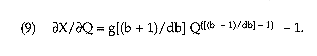
How Cocaine Consumption Varies With Seizures
Equation (8) reveals how equilibrium cocaine consumption Q varies with magnitude X of seizures. Under (8), the derivative of X with respect to Q is
Hence, the derivative of Q with respect to X, evaluated at a specified value of Q, is
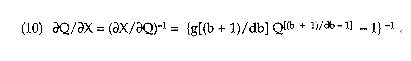
The complexity of the expression on the right side of (10) shows that it is not a simple matter to characterize the quantitative response of co-
caine consumption to seizures. The magnitude of the derivative ∂Q/∂X depends on the shape of the demand function as controlled by the demand elasticity parameter b, on the shape of the cost function as controlled by the power-function parameter d, and on the composite parameter g, as well.
We wish to focus here on the role played by parameter d, determining the shape of the cost function. For this purpose, it simplifies matters to choose certain values for the other parameters. In particular, suppose that b = -0.5 and that a = c = 1. The value b = -0.5 is the RAND baseline value for the demand elasticity. Setting a = c = 1 implies that g = 1. With these choices for (a, b, c), equations (8) and (10) reduce to
and
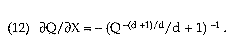
Observe that setting X = 0 in equation (11) yields Q = 1 as the equilibrium consumption of cocaine for all values of the parameter d. Evaluating the derivative (12) at the point Q = 1 reveals how consumption falls as seizures rise above zero. The result is

Thus, the response of cocaine consumption to seizures increases with the value of d. Under the RAND assumption that d = 1, consumption of cocaine responds least to seizures. The derivative value (∂Q/∂X)Q=1 = -1/2 that holds in this case implies that, as seizures rise from 0 equilibrium cocaine consumption falls by half the amount seized. In contrast, if the value of d is much larger than 1, then the derivative (∂Q/∂X)Q=1 is close to -1, implying that equilibrium cocaine consumption falls by almost all the amount seized.
In the market simulation in Figure 2 (in Section 2 of report), the parameter d is set to 1 to produce the two downward sloping average cost curves and to 4 to produce the two upward sloping average cost curves. These values for d are selected to illustrate the sensitivity of predictions to the assumed shape of the average cost curve. The actual shape of the curve is unknown.


