
C
Assessing Prevalence of Inadequate Intakes for Groups: Statistical Foundations
This appendix provides the formal statistical justification for the methods for assessing the prevalence of inadequate intakes that were described in Chapter 4. Additional details can be found in Carriquiry (1999).
Let Yij denote the observed intake of a dietary component on the jth day for the ith individual in the sample, and define yi= E{Yij| i} to be that individual's usual intake of the component. Further, let ri denote the requirement of the dietary component for the ith individual. Conceptually, because day-to-day variability in requirements is typically present, ri is defined as = E{Rij| i} and, as in the case of intakes, Rij denotes the (often unobserved) daily requirement of the dietary component for the ith individual on the jth day. In the remainder of this appendix, usual intakes and usual requirements are simply referred to as intakes and requirements, respectively.
The problem of interest is assessing the proportion of individuals in the group with inadequate intake of the dietary component. The term inadequate means that the individual's usual intake is not meeting that individual's requirement.
THE JOINT DISTRIBUTION OF INTAKE AND REQUIREMENT
Let FY,R (y,r) denote the joint distribution of intakes and requirements, and let ƒY,R (y,r) be the corresponding density. If ƒY,R (y,r) (or a reliable density estimate) is available, then
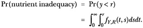 (1)
(1)
For a given estimate of the joint distribution ƒY,R, obtaining equation 1 is trivial. The problem is not the actual probability calculation but rather the estimation of the joint distribution of intakes and requirements in the population.
To reduce the data burden for estimating ƒY,R, approaches such as the probability approach proposed by the National Research Council (NRC, 1986) and the Estimated Average Requirement (EAR) cut-point method proposed by Beaton (1994), make an implicit assumption that intakes and requirements are independent random variables —that what an individual consumes of a nutrient is not correlated with that individual's requirement for the nutrient. If the assumption of independence holds, then the joint distribution of intakes and requirements can be factorized into the product of the two marginal densities as follows:
ƒY,R(r, y) = ƒR(r)ƒY(y) (2)
where ƒY(y) and ƒR(r) are the marginal densities of usual intakes of the nutrient, and of requirements respectively, in the population of interest.
Note that under the formulation in equation 2, the problem of assessing prevalence of nutrient inadequacy becomes tractable. Indeed, methods for reliable estimation of ƒY(y) have been proposed (e.g., Guenther et al., 1997; Nusser et al., 1996) and data are abundant. Estimating ƒR(r) is still problematic because requirement data are scarce for most nutrients, but the mean (or perhaps the median) and the variance of ƒR(r) can often be computed with some degree of reliability (Beaton, 1999; Beaton and Chery, 1988; Dewey et al., 1996; FAO/WHO, 1988; FAO/WHO/UNU, 1985). Approaches for combining ƒR(r) and ƒY(y) for prevalence assessments that require different amounts of information (and assumptions) about the unknown requirement density ƒR(r) and the joint distribution FY,R(y, r) are discussed next.
THE PROBABILITY APPROACH
The probability approach to estimating the prevalence of nutrient inadequacy was proposed by the National Research Council (NRC, 1986). The idea is simple. For a given a distribution of requirements in the population, the first step is to compute a risk curve that associates intake levels with risk levels under the assumed requirement distribution.
Formally, the risk curve1 is obtained from the cumulative distribution function (cdƒ) of requirements. If we let FR(.) denote the cdƒ of the requirements of a dietary component in the population, then
FR(a) = Pr(requirements ≤ a)
for any positive value a. Thus, the cdƒ FR takes on values between 0 and 1. The risk curve ρ (.) is defined as
ρ(a)=l − FR(a)=l − Pr(requirements ≤ a)
A simulated example of a risk curve is given in Figure 4-3. This risk curve is easy to read. On the x-axis the values correspond to intake levels. On the y-axis the values correspond to the risk of nutrient inadequacy given a certain intake level. Rougher assessments are also possible. For a given range of intake values, the associated risk can be estimated as the risk value that corresponds to the midpoint of the range.
For assumed requirement distributions with usual intake distributions estimated from dietary survey data, how should the risk curves be combined?
It seems intuitively appealing to argue as follows. Consider again the simulated risk curve in Figure 4-3 and suppose the usual intake distribution for this simulated nutrient in a population has been estimated. If that estimated usual intake distribution places a very high probability on intake values less than 90, then one would con-
|
1 |
When the distribution of requirements is approximately normal, the cdƒ can be easily evaluated in the usual way for any intake level a. Let z represent the standardized intake, computed as z = (a − mean requirement) / SD, where SD denotes the standard deviation of requirement. Values of FR(z) can be found in most statistical textbooks, or more importantly, are given by most, if not all, statistical software packages. For example, in SAS, the function probnorm (b) evaluates the standard normal cdƒ at a value b. Thus, the “drawing the risk curve” is a conceptualization rather than a practical necessity. |
clude that most individuals in the group are likely to have inadequate intake of the nutrient. If, on the other hand, the usual nutrient intake distribution places a very high probability on intakes above 90, then one would be confident that only a small fraction of the population is likely to have inadequate intake. Illustrations of these two extreme cases are given in Figure 4-4 and Figure 4-5.
In general, one would expect that the usual intake distribution and the risk curve for a nutrient show some overlap, as in Figure 4-6. In this case, estimating the portion of individuals likely to have inadequate intakes is equivalent to computing a weighted average of risk, as explained below.
The quantity of interest is not the risk associated with a certain intake level but rather the expected risk of inadequacy in the population. This expectation is based on the usual intake distribution for the nutrient in the population. In other words, prevalence of nutrient inadequacy is defined as the expected risk for the distribution of intakes in the population. To derive the estimate of prevalence, we first define
-
p(y) as the probability, under the usual intake distribution, associated with each intake level y and
-
ρ(y) as the risk calculated from the requirement distribution. The calculation of prevalence is simple
![]() (3)
(3)
where, in practice, the sum is carried out only to intake levels where the risk of inadequacy becomes about zero.
Notice that equation 3 is simply a weighted average of risk values, where the weights are given by the probabilities of observing the intakes associated with those risks. Formally, the expected risk is given by
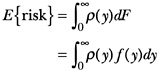
where ρ(y) denotes the risk value for an intake level y, F is the usual
intake distribution, and ƒ(y) is the value of the usual intake density at intake level y.
When the NRC proposed the probability approach in 1986, statistical software and personal computers were not as commonplace as they are today. The NRC included a program in the report that could be used to estimate the prevalence of nutrient inadequacy using the probability approach. As an illustration, the NRC also mentioned a simple computational method: rather than adding up many products ρ(y) p(y) associated with different values of intakes, intakes are grouped by constructing m bins. The estimated probabilities associated with each bin are simply the frequencies of intakes in the population that “fall into” each bin. (These frequencies are determined by the usual intake distribution in the population.) The average risk associated with intakes in a bin is approximated as the risk associated with the midpoint of the bin. An example of this computation is given on page 28, Table 5-1, of the NRC report (1986). Currently, implementation of the probability approach can be carried out with standard software (such as BMDP, SAS, Splus, SPSS, etc.).
In general, researchers assume that requirement distributions are normal, with mean and variance as estimated from experimental data. Even under normality, however, an error in the estimation of either the mean or the variance (or both) of the requirement distribution may lead to biased prevalence estimates. NRC (1986) provides various examples of the effect of changing the mean and the variance of the requirement distribution on prevalence estimates. Although the probability approach was highly sensitive to specification of the mean requirement, it appeared to be relatively insensitive to other parameters of the distribution as long as the final distribution approximated symmetry. Thus, although the shape of the requirement distribution is clearly an important component when using the probability approach to estimate the prevalence of nutrient inadequacy, the method appears to be robust to errors in shape specifications.
The NRC report discusses the effect of incorrectly specifying the form of the requirement distribution on the performance of the probability approach to assess prevalence (see pages 32–33 of the 1986 NRC report), but more research is needed in this area, particularly on nonsymmetrical distributions. Statistical theory dictates that the use of the incorrect probability model is likely to result in an inaccurate estimate of prevalence except in special cases. The pioneering efforts of the 1986 NRC committee need to be contin-
ued to assess the extent to which an incorrect model specification may affect the properties of prevalence estimates.
THE EAR CUT-POINT METHOD
The probability approach described in the previous section is simple to apply and provides unbiased and consistent estimates of the prevalence of nutrient inadequacy under relatively mild conditions (i.e., intake and requirement are independent, distribution of requirement is known). In fact, if intakes and requirements are independent and if the distributions of intakes and requirements are known, the probability approach results in optimal (in the sense of mean squared error) estimates of the prevalence of nutrient inadequacy in a group. However, application of the probability approach requires the user to choose a probability model (a probability distribution) for requirements in the group. Estimating a density is a challenging problem in the best of cases; when data are scare, it may be difficult to decide, for example, whether a normal model or a t model may be a more appropriate representation of the distribution of requirements in the group. The difference between these two probability models lies in the tails of the distribution; both models may be centered at the same median and both reflect symmetry around the median, but in the case of t with few degrees of freedom, the tails are heavier, and thus one would expect to see more extreme values under the t model than under the normal model. Would using the normal model to construct the risk curve affect the prevalence of inadequacy when requirements are really distributed as t random variables? This is a difficult question to answer. When it is not clear whether a certain probability model best represents the requirements in the population, a good alternative might be to use a method that is less parametric, that is, that requires milder assumptions on the t model itself. The Estimated Average Requirement (EAR) cut-point method, a less parametric version of the probability approach, may sometimes provide a simple, effective way to estimate the prevalence of nutrient inadequacy in the group even when the underlying probability model is difficult to determine precisely. The only feature of the shape of the underlying model that is required for good performance of the cut-point method is symmetry; in the example above, both the normal and the t models would satisfy the less demanding symmetry requirement and therefore choosing between one or the other becomes an unnecessary step.
The cut-point method is very simple: estimate prevalence of inad-
equate intakes as the proportion of the population with usual intakes below the median requirement (EAR).
To understand how the cut-point method works, the reader is referred to Chapter 4, where the joint distribution of intakes and requirements is defined. Figure 4-8 shows a simulated joint distribution of intakes and requirements. To generate the joint distribution, usual intakes and requirements for 3,000 individuals were simulated from a χ2 distribution with 7 degrees of freedom and a normal distribution, respectively. Intakes and requirements were generated as independent random variables. The usual intake distribution was rescaled to have a mean of 1,600 and standard deviation of 400. The normal distribution used to represent requirements had a mean of 1,200 and standard deviation of 200. Note that intakes and requirements are uncorrelated (and in this example, independent) and that the usual intake distribution is skewed. An individual whose intake is below the mean requirement does not necessarily have an inadequate intake.
Because inferences are based on joint rather than the univariate distributions, an individual consuming a nutrient at a level below the mean of the population requirement may be satisfying the individual 's own requirements. That is the case for all the individuals represented in Figure 4-8 by points that appear below the 45° line and to the left of the vertical EAR reference line, in triangular area B.
To estimate prevalence, proceed as in equation 1, or equivalently, count the points that appear above the 45° line (the shaded area), because for them y < r. This is not a practical method because typically information needed for estimating the joint distribution is not available. Can this proportion be approximated in some other way? The probability approach in the previous section is one such approximation. The EAR cut-point method is a shortcut to the probability approach and provides another approximation to the true prevalence of inadequacy.
When certain assumptions hold, the number of individuals with intakes to the left of the vertical intake = EAR line is more or less the same as the number of individuals over the 45° line. That is,
or equivalently,
Pr{y ≤ r} ≈ Fr(a)
where FY(a) = PR{y ≤ a} is the cdf of intakes evaluated at a, for a = EAR In fact, it is easy to show that when E(r) = E(y):
Pr(y ≤ r)= FY(EAR)
The prevalence of inadequate intakes can be assessed as long as one has an estimate of the usual nutrient intake distribution (which is almost always available) and of the median requirement in the population, or EAR, which can be obtained reliably from relatively small experiments.
The quantile FY(EAR) is an approximately unbiased estimator of Pr{y ≤ r} if
-
ƒY,R(y,r) = fY(y) fR(r), that is intakes and requirements are independent random variables.
-
Pr{r ≤ –α} = Pr{r ≥ α} for any α > 0, that is, the distribution of requirements is symmetrical around its mean; and
-
 >
>  , where and denote the variance of the distribution of requirements and of intakes, respectively.
When any of the conditions above are not satisfied, FY(EAR) ≠ Pr{y ≤ r}, in general. Whether FY (EAR) is biased upward or downward depends on factors such as the relative sizes of the mean intake and the EAR.


