
Appendix E An Economic Model of Supply and Demand for Teachers
Teacher licensure testing affects the quantity and quality of teachers through its effect on the supply of and demand for teachers. An analysis of the costs and benefits associated with teacher licensure testing, therefore, requires an understanding of the determinants of supply and demand.
THE SUPPLY OF TEACHERS
To fix ideas, we first present an analysis of teacher supply in the case where there is no licensure testing. In both cases, with and without licensure testing, it is assumed that in the general population of potential teachers the proportion who would be competent as teachers is given by qc (and the proportion who would not by qI=1−qc). This assumption is in keeping with the notion that licensure tests are designed to distinguish only among the two groups: those who are competent (with respect to the skills that are measured by the test) and those who are not. In what follows, we refer to the two types of individuals, would be competent teachers and would be incompetent teachers, as belonging to group C and group I, respectively.
No Licensure Testing
A simple model of occupational choice is adopted here in which an individual chooses among occupations according to which provides the greater compensation (wage).1 The wage offered to teachers in a given labor market is
denoted by w and, because competency is assumed to be indeterminate without a test or for institutional reasons, the wage offer is assumed to be the same regardless of whether the teacher is competent or not.2 However, the wages of individuals outside of teaching do differ. In particular, individuals who would be competent teachers have a wage distribution in alternative occupations with a given mean of wCa and individuals who would be incompetent teachers have a distribution with mean wage wIa.
Individuals choose teaching versus an alternative occupation depending on which provides the higher wage. Thus, an individual k in group C who would command a wage of wCka in a nonteaching occupation chooses teaching if and only if w>wCka=wCa+εCka, where εCka reflects the deviation of the individual’s wage from the mean wage of group C. Analogously, an individual j in group I would choose teaching if and only if w>wIia=wIa+εIia, where εIia reflects the deviation of the individual’s wage from the mean wage of group I. Given these rules for choosing an occupation, the probability that an individual in group C chooses teaching is given by αC=Pr(εCka<w−wCa). Likewise, the probability that an individual in group I chooses teaching is αI=Pr(εIia<w−wIa). From these definitions it is easy to see that the proportion of individuals who choose to be teachers at any given wage is qCαC+(1−qC)αI, and the proportion of them who would be competent teachers is ΠC=qCαC/[qCαC+(1−qC)αI].
As the wage paid to teachers increases, teaching becomes more attractive to both groups (both αC and αI are increasing in the wage, w). However, it is not possible to determine whether the proportion of teachers who are competent increases or decreases as the wage paid to teachers increases. The effect of the wage on the relative supply of competent teachers, that is, on ΠC, depends on the level of the wage paid to teachers and on how the distribution of wage offers in alternative occupations differs between the two groups. In the analysis that follows, it is assumed that the wage paid to teachers is in a range such that the proportion of competent teachers does not change with the wage, that is, ΠC is independent of w.
Figure E-1 shows the supply of teachers as a function of the wage paid to teachers. The number of teachers, denoted by T, is increasing with the teachers’ wage. The proportion of competent teachers (at wage w0 and, by assumption, at any wage) is given by E0/T0.
Licensure Testing
Assume now that all potential teachers must take a licensure test. The purpose and design of the test are to distinguish between the two groups, which it
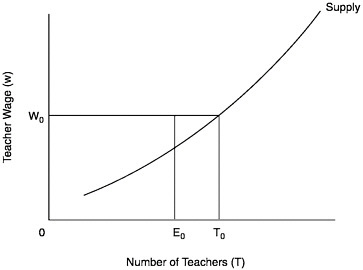
FIGURE E-1 The supply of teachers: no licensing test.
NOTES:
T0=number of individuals who would choose the teaching occupation at wage W0;
E0=number of individuals in group C who would choose the teaching occupation at wage W0.
may do with varying success. To capture the imperfect nature of tests, let mI and mC be the proportions of incompetent and competent individuals, respectively, who are classified as incompetent.3 Thus, if the test could discriminate perfectly, mI would be one (all those from group I would be determined to be incompetent) and mC would be zero (none of those from group C would be determined to be incompetent). It is reasonable to assume that mI exceeds mC for current licensing tests, although the extent to which this is true is unknown and may differ among both the type of skills that are tested (basic skills, subject matter knowledge, pedagogical content knowledge) and among different tests of the same skills.
Further, assume that a cost must be incurred to take the test, including both a monetary cost, which is the same for both groups, and a cost in terms of the effort involved in preparing for the test, which may differ between the two groups.4 These costs are denoted by tI and tC. Although stronger than necessary,
it is also assumed that individuals know to which group they belong (but the licensing authority does not, which is the rationale for the test).
When there is a licensure test, an individual can choose only whether or not to take the test. Becoming a teacher depends on whether one passes the test, that is, whether one is classified as competent or not. Given this framework, an individual k from group C chooses to take the licensure test if and only if w−tC/[1−mC]> wCa+εCka.5 Similarly, an individual j from group I chooses to take the test if and only if w−tI/[1−mI]>wIa+εIja. As in the case of no licensure testing, define αC=Pr(w−tC/[1−mC]−wCa>εCka) and αI=Pr(w−tI/[1−mI]−wIa>εIka) to be the probabilities that the group C and group I individuals choose to take the test, respectively.
Note that the relevant (effective) cost of the test in making this decision is the actual cost divided by the probability of being determined to be competent. Thus, for example, if the test were perfect (mI=1 and mC=0), only individuals from group C would decide to take it (group I individuals essentially face an infinite cost) and all of them would pass and become teachers. In general, increasing the probability that individuals will be found to be incompetent, regardless of the group, reduces the number of individuals who choose to take the test, which reduces the supply of teachers.
With an imperfect licensure test, the supply of both types, those who would be as well as those who would not be competent teachers, is lower than if there were no licensure test. There are two reasons for this result. The first is mechanical. Individuals who fail the test are simply precluded from choosing to be a teacher. To the extent that some group C individuals are misclassified by the test (mC>0), the supply of competent teachers will be reduced. The second reason is due to behavior. The cost of the test makes the teaching occupation relatively less attractive than alternative occupations, and, as in the first reason, misclassifying competent people (mC>0) increases that cost and reduces their supply.
Formally, the supply of competent teachers is qC(1−mC)αC and the supply of incompetent teachers is qI(1−mI)αI, with the total supply of teachers given by their sum. The proportion of teachers who are competent at some given wage is, therefore, ΠC=qC(1−mC)αC/[qC(1−mC)αC+qI(1−mI)αI]. As in the
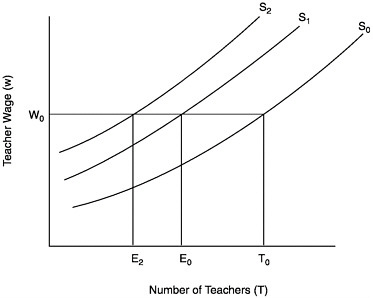
FIGURE E-2 The supply of teachers: perfect licensing test.
NOTES:
S0=supply of teachers when there is no licensure tests;
S1=supply of teachers when tests are not costly;
S2=supply of teachers when tests are costly;
T0=number of individuals who would choose the teaching occupation at wage W0;
E0=number of individuals in group C who would choose the teaching occupation at wage W0;
E2=number of individuals in group C who would choose the teaching occupation at wage W0 when tests are costly.
no-licensure case, it is assumed that ΠC is independent of the wage. However, the proportion of competent teachers is directly related to the efficiency of the test in distinguishing between the two types and to the cost of the test for the two reasons given above.
Figure E-2 depicts the supply of teachers in the case of a perfect test as compared to the no-test case shown in Figure E-1. The supply curve labeled S0 corresponds to the no-test case. Recall that E0 is the number of individuals in group C who would choose the teaching occupation. The supply curve corresponding to S1 shows the supply of teachers when there is a license test but when its cost is zero. In that case, at each wage all of the teachers are competent. S2 shows the supply of teachers when the test is costly. In that case, as when the test is not costly, all of the teachers are competent, but there are fewer at any wage
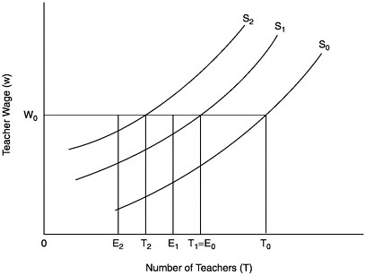
FIGURE E-3 The supply of teachers: imperfect licensure test.
NOTES:
S0=supply of teachers when there is no licensure test; S1=supply of teachers when tests are not costly;
S2=supply of teachers when tests are costly;
T0=number of individuals who would choose the teaching occupation at wage W0;
T1=number of individuals who would choose the teaching occupation at wage W0 when tests are not costly, and who pass the test;
T2=number of individuals who choose the teaching occupation at wage W0 when tests are costly and who pass the test;
E1=number of individuals in group C who choose the teaching occupation at wage W0 when tests are not costly and who pass the test;
E2=number of individuals in group C who choose the teaching occupation at wage W0 when tests are costly and who pass the test.
who choose to be teachers. Thus, even a perfect licensure test will lead to a reduction in the supply of competent teachers if the test is costly.6
Figure E-3 shows the intermediate case, where the test is imperfect, that is, where there are type 1 and type 2 errors. The original no-test supply is again
shown as the baseline case. S1, as before, shows the supply of teachers when there is a test, but the test is not costly. In that case the number of teachers at wage w0 is assumed to be T1 (which, for illustrative purposes, is depicted as being equal to E0, the number of competent teachers when there is no test). Note that the only reason for this reduction in supply is due to the mechanical feature of the test. However, because an imperfect test does not correctly identify all of the incompetent teachers from group I, only E1 of the T1 teachers are competent. However, under the maintained assumption that mI exceeds mC, the fraction of teachers who are competent is increased through the use of the test, that is E1/T1>E0/T0. With a costly test, the number of teachers falls further to T2 at the wage w0. In addition, if the (effective) cost of the test is higher for the incompetent, there will be a tendency for the proportion of teacher who are competent among the T2 teachers to rise further. Thus, an imperfect licensure test will reduce the number of competent teachers but by less than the overall supply of teachers.
Raising Passing Scores
The same analysis would apply to raising passing scores on existing licensure tests. In Figure E-3, let S0 be the supply curve associated with an existing (imperfect) licensure test, say one with a low passing score. A test with a low passing score will tend to have only a small supply effect (relative to a no-licensure test regime) as the proportion of individuals in both groups taking the test who are determined to be incompetent will be small (mI and mC are both small). Increasing the passing score will tend to increase both mI and mC. To the extent that mI increases faster than mC, the relative number of competent teachers will tend to increase, although the supply (at a given wage) of both competent and incompetent teachers will fall. As passing scores are continually raised, however, it becomes more and more likely that the supply of competent teachers falls by more than does the supply of incompetent teachers. When potential teachers are mostly competent, increasing passing scores will eliminate mostly competent teachers.
If nothing else changes when licensure tests are used or passing scores are raised, in particular, if the wage to teachers is not affected by the reduction in supply, class size will rise. Whether overall student learning increases or decreases would depend on whether students are better off with competent teachers in larger classes or with a mix of competent and incompetent teachers in smaller classes. But wages are unlikely to be unchanged. To see that, the demand for teachers must be modeled.
THE DEMAND FOR TEACHERS
The model of demand, like that of supply, is illustrative. Only an outline of the model is presented here, and the basic conclusions are stated. Consider a
school district in a municipality that supplies not only educational services but other local public goods. The municipality, for given tax revenues, decides on the amount to spend on education, whose only variable input is the number of teachers, and spends the residual amount on the other local public goods.7
Student learning is assumed to depend only on the number of competent teachers; incompetent teachers produce no learning.8 It is thus assumed that reducing the number of teachers if they come solely from the set of incompetent teachers will not reduce student learning even though the number of students per competent teacher (class size) rises.9 The school district (or equivalently the municipality) takes teachers’ wages as given; that is, it must compete with other municipalities for teachers in the same labor market. Like the wage, the municipality also takes as given the fraction of teachers who are competent. The municipality maximizes a community welfare function that depends on student learning and on the amount of other local public goods that it purchases for the community.
Maximizing community welfare leads to a demand function for teachers (derived from the demand for student learning) that depends on the competitively determined market wage and on the fraction of competent teachers (which we assumed above to be independent of the wage offered to teachers) in the total supply. As usual, it can be shown that the demand for teachers is declining with the teacher wage. In addition, the demand for teachers can either rise or fall at any given wage as the proportion of competent teachers in the total supply of teachers increases. However, the demand for competent teachers at any give wage must rise with an increase in the proportion of competent teacher in the total supply. The importance of this last result will become clear below. The market demand for teachers is the (horizontal) sum of the demand across municipalities in the same teacher labor market.
THE EQUILIBRIUM TEACHER WAGE AND NUMBER OF COMPETENT TEACHERS
The equilibration of market demand and supply determines the teacher wage and the number of teachers who are employed. Given the proportion of teachers
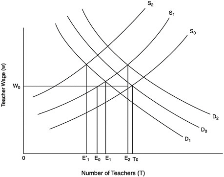
FIGURE E-4 Equilibrium in the market for teachers: perfect licensure test.
NOTES:
S0=supply of teachers when there is no licensure test;
S1=supply of teachers when tests are not costly;
S2=supply of teachers when tests are costly;
D0=market demand for teachers when there is no licensure test;
D1=market demand for teachers when all individuals who pass the test are competent Case I;
D2=market demand for teachers when all individuals who pass the test are competent Case 2;
T0=Number of individuals who choose the teaching occupation at wage W0;
E0=Number of individuals who choose the teaching occupation at wage W0;
E1=Number of individuals in group C employed as teachers when tests are not costly and when demand is given by D1;
E2=Number of individuals in group C employed as teachers when tests are not costly and when demand is given by D2;
E′1=Number of individuals in group C employed as teachers when tests are costly and when demand is given by D1.
who are competent, that is, given the properties of the licensing test, the number of teachers who are competent is also determined.10
Figure E-4 considers the case of a perfect licensure test, incorporating market demand into Figure E-2. Recall that a perfect test has the property that all those who pass it are competent and all those who do not pass are not competent. D0 represents market demand for teachers when there is no licensure test. The equilibrium wage is w0, the equilibrium number of teachers is T0, and the number of competent teachers is E0. S1 represents the supply when the test is costless. As seen, if the wage remained at its original equilibrium, the number of teachers would be E0 and the fraction of competent teachers would be one (all teachers are competent with a perfect test). However, given that the fraction of competent teachers is one, independent of the wage, the demand curve may shift either up or down. The model tells us only that the demand will not shift down so much that the number of competent teachers falls below what it was in the baseline no-licensure case. Regardless of the direction in which demand shifts, the wage paid to teachers will rise, but this new wage simply reflects the appropriate scarcity of competent teachers. Because the number of competent teachers rises, student achievement also rises.
With a costly test, the supply of teachers shifts further to S2. There is no further shift in the demand for teachers (the proportion of competent teachers is still one). In this case it is possible that if the test is costly enough the number of competent teachers will actually fall, for example, from E0 to E1?. Even in a less extreme case in which the number of competent teachers rises and thus so does student learning, it is possible that the municipality would be better off without the test given the higher wage that must be paid to teachers.11 However, recall that in the case of a perfect test, only group C individuals take the test and the effective cost is the same as the actual cost. If the cost of the test to the competent group can be considered small, a perfect test would not contain this inefficiency. The more imperfect the test, the more likely the test is to reduce community welfare.
Setting Passing Scores
The same analysis also applies to the case where the test classifies all group I individuals correctly but some of those from group C are mistakenly classified
as not competent (type 2 error). This outcome could arise if the test is inherently imperfect in the sense that there does not exist a passing score for which there are no classification errors or because the test would be perfect at a specific passing score but the passing score is set at too high a level. As with a perfect test, only group C individuals take the test, but unlike the perfect test some of them fail. In this case, the shift (fall) in supply is larger than that depicted in Figure E-4 by the movement from S0 to S1, even when the test is costless. Depending on how big this type 2 error is, the number of competent teachers may fall below the number when there is no licensure test. Even if the result is not that extreme, this restriction on supply leads to an artificially high wage that might not be the most efficient way to spend community resources.
The analysis of passing scores is more complicated when the test is imperfect in the sense of having both type 1 and type 2 errors. Setting a low passing score may increase the proportion of competent teachers only slightly relative to the situation without a test, but it protects against artificially restricting the supply of competent teachers. Setting a high passing score may increase the proportion of competent teachers a great deal but risks reducing significantly the number of competent teachers and artificially increasing the wage. As the prior discussion makes clear, quantitatively assessing the efficacy of licensure testing requires a great deal of information, about not only the accuracy of the test but also the perceived costs to the test takers, alternative market opportunities of potential teachers, and constraints on the tax revenues of municipalities.


