
Calibration in Computer Models for Medical Diagnosis and Prognostication
LUCILA OHNO-MACHADO
University of California, San Diego
FREDERIC RESNIC
Brigham and Women’s Hospital and Harvard Medical School
Cambridge, Massachusetts
MICHAEL MATHENY
Vanderbilt University
Nashville, Tennessee
Predictive models to support diagnoses and prognoses are being developed in virtually every medical specialty. These models provide individualized estimates, such as a prognosis for a patient with cardiovascular disease, based on specific information about that individual (e.g., genotype, family history, past medical history, clinical findings). Statistical and machine-learning techniques applied to large clinical data sets are used to develop the models, which are used by both health care professionals and patients. However, verification (a critical step in the evaluation of a model) that the probabilities of estimated or predicted events truly reflect the underlying probability for a particular individual is often overlooked.
ASSESSING CALIBRATION
A simplistic type of calibration is calibration-in-the-large or bias. If the outcome is binary (e.g., “0” if a patient is not diseased and “1” if a patient is diseased), the bias corresponds to the average error for the estimates. For example, an estimate of 89 percent for a patient whose outcome is “1” contributes an individual error of 0.11. The average error for all patients is the measure of calibration-in-the-large. Calibration-in-the-large may be appropriate for considering a group of patients, but says little about how calibrated each estimate is. For example, the assignment of the prior probability of an event as the estimate or risk score for every patient, although it would result in a perfectly calibrated-in-the-large model,
would provide no individualized information. Hence it would be of limited practical utility for assessing predictive models.
A fundamental problem in evaluating the calibration of a model in a health care setting is the lack of a gold standard against which individual risk estimates can be compared. A gold standard would be based on a sufficient number of exact replicas of the individual, accurately diagnosed or followed without censoring, so that the proportion of observed events would be equal to the “true estimate” for that individual.
Since every individual is unique, meaningful approximations of true probability are only possible for relatively large groups of similar individuals. However, the way the similarity of patient profiles is defined is a critical factor. Currently, calibration is measured by comparing health outcomes in sets of patients with similar estimated risks. That is, given a predicted risk for an individual, a set of neighboring individuals (in the sense of proximity in single dimension of the estimates, or “output space”) is assembled and the bias for this set is assessed. This measure of “calibration-in-the-small” is the same as the measure of “calibration-in-the-large,” except that it is applied to a smaller set based on individuals who received similar estimates by a given model.
OUTPUT-SPACE SIMILARITY
One of the most widely used indices in assessing calibration of predictive models was developed in the context of logistic regression by Lemeshow and Hosmer (1982). The idea behind the test is simple: if cases are sorted according to their estimated level of risk and the mean estimate for each decile of risk is very close to the proportion of positive cases in the decile, then one cannot reject the hypothesis that the model is correct (Hosmer and Hjort, 2002; Hosmer et al., 1991, 1997). The sum (i.e., the squared differences between the sum of estimates and number of events in each decile divided by the sum of estimates in that decile) for each outcome is reported to follow a χ2 distribution with 8 degrees of freedom. If p < 0.05, we reject the hypothesis that the model fits the data. The H-L-C statistic based on deciles of risk is defined as:
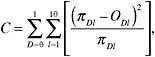
where πDl and oDl are the sum of estimates in a decile and observed frequencies in the same decile, for cells indexed by group (decile) l and outcome D. Hosmer and Lemeshow showed via simulations that C is approximately distributed as χ2 with l-2 = 8 degrees of freedom when the fitted model is the correct one and the estimated expected cell frequencies are sufficiently large.
Note that the H-L statistic is model-dependent because the statistic compares
the average estimate in each decile of estimated risk with the proportion of events in that decile. To visualize the calibration of a predictive model, it is common to plot the average estimate for groups representing either (1) percentiles of estimated risk against the proportion of events in that group, as described above, or (2) pre-defined ranges of the estimates. The latter is commonly used in clinical predictive models.
INPUT-SPACE SIMILARITY
We described above how output-space similarity can be used to measure calibration in a more refined way. However, output-space similarity is model-dependent and difficult to understand. Similarity at the input-space is much simpler (e.g., calculation of neighborhoods using features obtained directly from data) and may be an equally legitimate way to assess calibration.
We describe a simulation in which we established in advance four tight clusters of “patients” (100 in each cluster) according to two variables, x1 and x2. The purposes of this simulation were to illustrate the H-L “goodness-of-fit” statistic and to check whether differences in calibration can be determined using this statistic. Bi-normal distributions were generated with identical standard deviations (0.1) and centered at (0,0), (0,1), (1,0), and (1,1) for clusters 1 to 4, respectively. The binary outcome for each patient in a cluster was generated from a Bernoulli distribution with probabilities 0.01, 0.4, 0.6, and 0.99 for clusters 1 to 4, respectively. Figure 1 shows the spatial distribution of the clusters. For verification, the four clusters were automatically re-discovered using the Expectation-Maximization algorithm.
The resulting logistic regression model is highly significant. For comparison, we built a neural network with hidden units so that it was capable of finding a non-linear function relating the predictors and outcomes (Figure 1b). An ideal model would assign the true underlying probability for each case (i.e., 0.01, 0.4, 0.6, and 0.99, depending on which cluster the case belonged to). A neural network with enough parameters was able to get closer to that goal than a semi-linear model, such as logistic regression.
Table 1 shows descriptive statistics for the estimates obtained by the two types of models. The H-L-C statistic for the logistic-regression model was 6.43 (p = 0.59); hence we would not reject the hypothesis that the model is calibrated. Although the neural network model had a less favorable H-L-C of 11.773 (p = 0.16), the overall errors were smaller.
In this example, the neural network provided better approximations of the true underlying probability of the event in clusters 2 and 3, as can be seen in the ranges of estimates in these clusters, as well as in their maximum residuals. However, comparison of H-L-C and the calibration plot (Figure 2) do not indicate that a neural network would be a better model in this case.
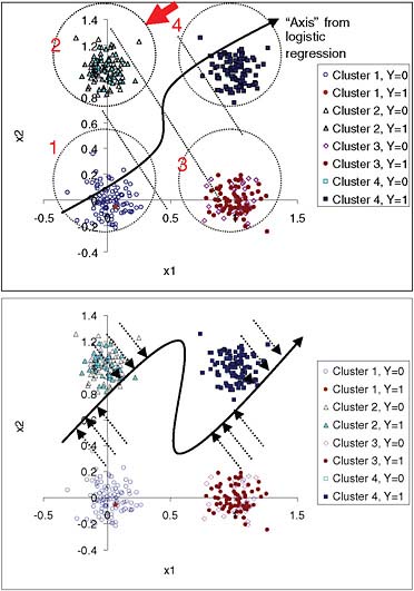
FIGURE 1 Simulation with four predefined non-overlapping bi-normal clusters of individuals with known underlying probability of an event (0.01, 0.40, 0.60, and 0.99 for clusters 1 to 4, respectively). Top panel: Two-dimensional data are projected into one dimension by the logistic-regression model. Dotted diagonal lines divide quartiles of risk. A patient from cluster 2, indicated by the arrow, has an estimate closer to the average estimate for cluster 3 than to the average for cluster 2. Confidence in this estimate should be lower than for a patient in the middle of one of the clusters. The input-space clusters, as opposed to the quartiles of risk, can be explained because patients in cluster 1 have low x1 and low x2, while patients in cluster 2 have low x1 and high x2, and so on. Bottom panel: Projection of the points into an “axis” for neural network estimates. The neural network model comes closer to the true probabilities for clusters 2 and 3 than the logistic-regression model.
TABLE 1 Descriptive statistics of logistic-regression (LR) and neural network (NN) estimates according to input-space clusters. Note that NN estimates do not overlap (i.e., the minimum estimate for cluster 3 is greater than the maximum estimate for cluster 2)
|
Cluster |
Proportion of Events |
LR Mean |
NN Mean |
LR Std Dev |
NN Std Dev |
LR Minimum |
NN Minimum |
LR Maximum |
NN Maximum |
|
1 |
0.01 |
0.0338 |
0.0219 |
0.0172 |
0.0069 |
0.0066 |
0.015 |
0.0949 |
0.059 |
|
2 |
0.42 |
0.4129 |
0.4819 |
0.1080 |
0.0207 |
0.1955 |
0.431 |
0.8013 |
0.584 |
|
3 |
0.64 |
0.6291 |
0.6852 |
0.1149 |
0.0146 |
0.2873 |
0.647 |
0.8507 |
0.732 |
|
4 |
0.98 |
0.9740 |
0.9908 |
0.0127 |
0.0011 |
0.9301 |
0.985 |
0.9954 |
0.992 |
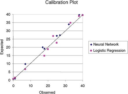
FIGURE 2 Calibration plot for logistic-regression and neural network models based on deciles of risk. There is no apparent superiority of one model over the other.
IMPLICATIONS FOR MEDICAL DECISIONS
In clinical practice, incorrect estimates have significant implications. For example, the widely used clinical practice guideline from the report by the Adult Treatment Panel III (NCEP, 2002) uses cardiovascular risk estimates similar to those available from online calculators to recommend particular treatment regimens. For non-calibrated estimates, this may result in the inappropriate use of medication to manage cholesterol levels.
Computer-based post-marketing tools for the surveillance of new medications and medical devices use models that adjust risk for the population being treated (Matheny et al., 2006). These models depend on the accuracy of the estimates to trigger appropriate alerts for unsafe technologies and drugs. For non-calibrated estimates, risk adjustments may result in a large number of false positives or of false negatives, either of which would incur large costs to the health care system. It is critical, therefore, to assess the calibration of estimates before using models in clinical settings.
We and others have shown, in different domains, that the calibration of medical diagnostic and prognostic models can vary significantly according to the
population to which they are applied (Hukkelhoven et al., 2006; Matheny et al., 2005; Ohno-Machado et al., 2006), even though discrimination indices such as the areas under the ROC curves may not vary. Although some efforts are being made to recalibrate models for different populations and study reclassification rates, Web-based calculators that estimate individualized risk do not yet take this issue into account and may present incorrect estimates for particular individuals.
We have proposed methods for taking into account input-space clusters in predictive models (Osl et al., 2008; Robles et al., 2008), but much remains to be done to inform health care workers and the public about the potential shortcomings of this aspect of personalized medicine. As new molecular-based biomarkers for a variety of health conditions are developed and used in multidimensional models to diagnose or prognosticate these conditions, it will become even more important to develop accurate methods of assessing the quality of estimates derived from predictive models.
ACKNOWLEDGMENTS
The authors acknowledge support from the National Library of Medicine, NIH, FDA, and VA grants R01LM009520 (LO), R01 LM008142 (FR), HHSF 223200830058C (FR), VA HSR&D CDA2-2008-020 (MM).VA HSR&D CDA2-2008-020 (MM).
REFERENCES
Hosmer, D.W., and N.L. Hjort. 2002. Goodness-of-fit processes for logistic regression: simulation results. Statistics in Medicine 21(18): 2723–2738.
Hosmer, D.W., T. Hosmer, S. Le Cessie, and S. Lemeshow. 1997. A comparison of goodness-of-fit tests for the logistic regression model. Statistics in Medicine 16(9): 965–980.
Hosmer, D.W., S. Taber, and S. Lemeshow. 1991. The importance of assessing the fit of logistic regression models: a case study. American Journal of Public Health 81(12): 1630–1635.
Hukkelhoven, C.W., A.J. Rampen, A.I. Maas, E. Farace, J.D. Habbema, A. Marmarou, L.F. Marshall, G.D. Murray, and E.W. Steverberg. 2006. Some prognostic models for traumatic brain injury were not valid. Journal of Clinical Epidemiology 59(2): 132–143.
Lemeshow, S., and D.W. Hosmer Jr. 1982. A review of goodness of fit statistics for use in the development of logistic regression models. American Journal of Epidemiology 115(1): 92–106.
Matheny, M.E., L. Ohno-Machado, and F.S. Resnic. 2005. Discrimination and calibration of mortality risk prediction models in interventional cardiology. Journal of Biomedical Informatics 38(5): 367–375.
Matheny, M.E., L. Ohno-Machado, and F.S. Resnic. 2006. Monitoring device safety in interventional cardiology. Journal of the American Medical Informatics Association 13(2): 180–187.
NCEP (National Cholesterol Education Program). 2002. Third report of the national cholesterol education program expert panel on detection, evaluation, and treatment of high blood cholesterol in adults (Adult Treatment Panel III) final report. Circulation 106(25): 3143–3421.
Ohno-Machado, L., F.S. Resnic, and M.E. Matheny. 2006. Prognosis in critical care. Annual Review of Biomedical Engineering 8: 567–599.
Osl, M., L. Ohno-Machado, and S. Dreiseitl. 2008. Improving calibration of logistic regression models by local estimates. AMIA Annuual Symposium Proceedings. 2008: pp. 535-539.
Robles, V., C. Bielza, P. Larranaga, S. Gonzales, and L. Ohno-Machado. 2008. Optimizing logistic regression coefficients for discrimination and calibration using estimation of distribution algorithms. TOP: An Official Journal of the Spanish Society of Statistics and Operations Research 16(2): 345–366.


