
Errata
Predicting Outcomes of Investments in Maintenance and Repair of Federal Facilities
APPENDIX C
NATIONAL RESEARCH COUNCIL
OF THE NATIONAL ACADEMIES
THE NATIONAL ACADEMIES PRESS
Washington, D.C.
ISBN-13: 978-0-309-22186-3; ISBN-10: 0-309-22186-2
NOTE TO READERS: Following the public release of this report in November 2011, errors were discovered in several of the equations and numerical solutions included in Appendix C. This document includes the corrected equations and solutions.
Copyright 2012 by the National Academy of Sciences. All rights reserved
Appendix C
Some Fundamentals of the Risk-Based Approach
BASIC PRINCIPLES
The fundamental tools needed for the quantitative risk-based approach to decision-making include the basic principles of probability. Those principles start with the premise that in the presence of uncertainty, a phenomenon or physical process can be defined or represented by a random variable and its probability distribution. That is, uncertainty is modeled as a random variable with a range of possible values and their probabilities defined by a probability distribution.
Thus, if X is a random variable with a range of possible values from a to b, its probability distribution may be defined as FX(x)=P(X≤x); a≤x≤b.
Within the range of possible values of a random variable, there will be a mean (or average) value and a measure of dispersion, such as the variance or standard deviation. The ratio of the standard deviation to the mean is the coefficient of variation (COV).
Among the useful probability distributions are the normal or Gaussian distribution and the lognormal (or logarithmic normal) distribution.
The Normal or Gaussian Distribution. The normal distribution, whose range of possible values is −∞ to +∞ is denoted as N(µ, σ), where µ is its mean value and σ is its standard deviation. If µ= 0 and σ= 1.0, the distribution is called the standard normal distribution. For the standard normal distribution, the probability from −∞ to x is FX(x)= Φ(x), where Φ(x) is tabulated in Tables of Standard Normal Probability. The probability of a random variable, X, between a and b can be evaluated as
![]()
where µX and σX are, respectively, the mean and standard deviation of X.
The Lognormal Distribution. In the lognormal distribution, whose range of possible values is 0 to ∞, there are no negative values. The probability that X will be between a and b becomes
![]()
where λX and ζX are, respectively, the mean and standard deviation of lnX and they are the parameters of the lognormal distribution. These parameters are related to the mean and standard deviation of X as follows:
![]()
and
![]()
if the COV of X, δX, is not large, say < 40%, ζ≅δ.X
MATHEMATICS OF PROBABILITY
A few rules that pertain to the mathematics of probability may be described briefly as follows.
Probability is defined with reference to the occurrence (or non-occurrence) of an event, and for an event E
0≤P(E)≤1.0
The Addition Rule. For two or more events, A and B, the “union” of A and B, denoted A∪B, means the occurrence of A or B (or both), and the probability is given as the addition rule namely
P(A∪B)=P(A)+P(B)-P(AB)
in which P(AB) stands for the simultaneous occurrence of A and B.
The Multiplication Rule. The probability of the simultaneous occurrence of two events, A and B, is given by the multiplication rule namely
![]()
in which ![]() stands for the “conditional probability” of A given (or assuming) the occurrence of B.
stands for the “conditional probability” of A given (or assuming) the occurrence of B.
Those two simple rules, together with the “theorem of total probability” and the “theorem of Bayes” constitute the basic rules of the mathematics of probability. For a more complete description of the theory of probability and illustrations of its many applications in engineering, see Ang and Tang (2007).
ILLUSTRATIVE APPLICATIONS TO SPECIFIC OUTCOMES
Described below are the numerical calculations of the risk or probability of “negative benefits” of three specific outcomes — accident rates and types, deferred maintenance, and energy use.
Accident Rates and Types
In this example, let
X = recordable incident rate (RIR)
Y = lost-time incident rate (LTR), and
Z = number of worker compensation claims
Assume that the current incident rates and claims are as follows:
X = 4 per 100,000 hours
Y = 0.5 per 100,000 hours
Z = 1
The average cost per incident and the average lost time cost per incident is $75,000, whereas that of a worker compensation claim is $100,000.
With an investment of $200,000 for maintenance and repair, the incident rates would be reduced as follows:
X’ = 2 per 100,000 hours
Y’ = 0.1 per 100,000 hours
Z’ = 0.2
In this case, the current cost of an incident is
C = c1X + c2Y + c3Z;
and the corresponding reduced cost is,
C’ = c1X’ + c2Y’ + c3Z’
where c1, c2, and c3 are the corresponding costs in dollars.
The pertinent costs are, therefore, as follows:
Current cost, C = 75,000 x 4 + 75,000 x0.5 + 100,000 x1 = $437,500
Reduced cost, C’ = 200,000 + 75,000 x 2 + 75,000 x 0.1 + 100,000 x 0.2 = $377,500
The benefit derived from the investment in maintenance and repair, therefore, would be
Benefit = C – C’. In this case, the benefit of maintenance and repair investment = 437,500 — $377,500 = $60,000
In this example, the risk that the investment will be greater than the savings (negative benefit) is C < C’. Because there are uncertainties in all the variables X, X’, Y, Y’, Z, and Z’, there is some probability of negative benefit. For example, suppose that the uncertainties are ±30% in all the variables. The risk would be calculated as follows.
Assume that the variables are independent normal random variables; the means and standard deviations of each of the variables are:
X = N(4, 1.2); Y = N(0.5, 0.15); Z = N(1, 0.3);
and X’ = N(2, 0.6); Y’ = N(0.1, 0.03); Z’ = N(0.2, 0.06)
The respective means of C and C’ (assuming no uncertainties in the costs), are
µC=$ 437,500 and µC’=$377,500
whereas the variances are,
![]()
and,
![]()
Therefore, the risk of negative benefit would be,
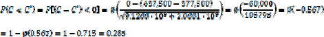
That means that with the investment of $200,000 in maintenance and repair, the risk of negative benefit will be about 28.5 percent.
Deferred Maintenance
Any equipment or facility has a finite and variable operational life. In realistic terms, the operational life may be represented as a random variable and described with a probability distribution. The probability distribution often used for this purpose is the lognormal distribution.
The Risk Problem
Consider the maintenance problem of air-conditioning (A/C) units. Assume that the operational life T of a typical A/C unit can be described with the lognormal distribution, with a median life of tm months or years, and a COV of δT (or a standard deviation of σT ≈ δT×tm).
Suppose further that the current maintenance schedule calls for inspection and repair (if necessary) of an A/C unit every n months or years. However, if inspection or repair is deferred beyond the schedule, what will be the reliability (probability of performance) of the A/C unit until the next scheduled inspection? And what would be the cost implication of deferring maintenance?
Solutions
Assume that the A/C unit has an operational life of tm = 5 years, and a COV of δT = 0.30. The probability that the A/C unit will fail to perform within a life of t years is given by P(T < t). With the lognormal distribution of the operational life T, the probability is
![]()
in which λ and ζ are the parameters of the lognormal distribution. The reliability is then (1 – P).
Problem I. The probability that the operational life of an A/C unit will be less than 2 years is determined as follows:
The parameters of the lognormal distribution λ and ζ are:
λ≈1ntm = 1n5 = 1.61; and ζ∼δT = 0.30.
The required probability of failure (non-performance) in 2 years is
![]()
Therefore, the probability that a typical A/C unit will fail within a 2-year period is 0.11 percent. Its reliability of performance, therefore, is (1 – 0.0011) = 0.9989 = 99.89 percent.
Problem II. Suppose that the A/C units of an agency are scheduled for routine maintenance at 2-year intervals; this maintenance schedule should ensure a high performance reliability (of 99.89 percent) However, because of circumstances (such as a shortage of technicians, or a shortage of funding), the inspection and repair schedule is deferred for 2 years (until the next scheduled maintenance).
The average cost of repair per A/C unit is estimated to be $1,500; the cost implication of the deferred maintenance will be as follows.
In this problem, the operational life is assumed to be longer than 2 years (the schedule for maintenance), so it is necessary to calculate the probability of failure in 4 years (2 years beyond the scheduled maintenance). The solution requires conditional probability as outlined below:
![]()
where, from Problem I,
P(T>2) = 1— 0.0011 0.9989
![]()
and
![]()
Therefore, deferring the maintenance of the A/C units for 2 years, or until the next scheduled maintenance, will result in a probability of failure of a typical A/C unit of 23 percent.
If the agency has 1,000 A/C units, 230 of them are likely to fail within 2 years beyond the scheduled maintenance. If the average repair cost is $1,500 per unit, the deferred maintenance cost will be 230 × 1500 = $345,000.
Energy Use
Problem
Determine the benefit of investments in maintenance and repair of energy systems. Consider savings in oil equivalents (gallons) of gasoline consumption at a price of $3.00 per gallon. Assume that with an investment of I (dollars) the reduction in gasoline consumption is Y = f(I); this function may have to be developed empirically from historical data.
Let the current consumption be X gallons; and in dollars = 3X.
Assume that with an investment of I dollars, the reduced consumption would be Y gallons, and in dollars = 3Y.
Therefore, the energy saving with investment I is (X – Y) gal; or in dollars is (3X – 3Y).
Hence, failure in this case may be defined as “saving (in dollars) is less than the investment”; that is, in dollars,
![]()
There will be uncertainty in X (the current consumption) and in Y (the reduced consumption), so there will be a probability of failure, or risk that the investment will be greater than the savings (negative benefit). To calculate that probability, assume that X and Y are both normal (or Gaussian) random variables, with respective means and standard deviations µX, µY, and σX, σY; i.e., denoted as
![]()
The probability of failure, P, is
![]()
For normal random variables, it becomes,
![]()
For numerical illustrations, assume hypothetically the following:
Current average gasoline consumption, is µX = 10 million gallons, with a standard deviation of σX = 2 million gallons.
With an investment of $10,000,000, the average reduced consumption is expected to be µY = 8 million gallons, and σY = 2 million gallons. The risk of a negative benefit is
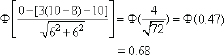
Therefore, with an investment of $10 million, there is a 68 percent probability of a negative benefit.
RELIABILITY ANALYSIS
The practical approach to ensure the reliability or safety of an engineered system is to apply the first-order reliability method (FORM). The basics of the method can be described below.
The evaluation of reliability of an engineered system may be considered as a problem of supply versus demand; for this purpose, define the following random variables:
X = the supply and
Y = the demand.
The objective of a reliability analysis is to insure that (X > Y).
If the probability density functions (PDFs) of X and Y are, respectively, fX(x) and fY(y), then the reliability of the system is measured by the probability of failure (non)performance),
![]()
in which,
![]()
The above is a convolution integral, shown graphically in Figure C.1.
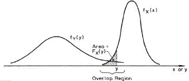
FIGURE C.1 The probability of failure.
The corresponding probability of performance is then
![]()
Consider a system in which the available supply, X, is a Gaussian or normal random variable N(µX, σX) and the demand is also a Gaussian random variable N(µY, σY). The difference, M = X – Y, called “safety margin”, is also a Gaussian variable with a mean of
![]()
If X and Y are statistically independent, the variance of M is ![]()
Furthermore, ![]() is N(0,1). Hence, the probability of
is N(0,1). Hence, the probability of
nonperformance is ![]()
in which Φ is the cumulative probability of the standard Gaussian distribution, N(0,1)
Clearly, the reliability of the system is a function of the ratio µM σM, which may be called the safety index or reliability index and denoted by β
In this case, ![]()
If the supply and demand are both lognormal random variables, the corresponding reliability index would be
![]()
and the probability of nonperformance can be expressed as
![]()
In the first case, where X and Y are both Gaussian random variables, the quantitative relation between pF and β is unique (one to one) as follows:
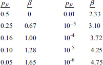
The First-Order Reliability Method (FORM)
Engineers are, traditionally, reluctant to admit a probability of failure; for this reason, a good alternative strategy is to use an equivalent measure, the safety index β – which is a complete measure of the safety or performance of an engineered system.
This has served to spur the practical implementation of the probabilistic approach in engineering.
Using the β and FORM has contributed greatly to the practical implementation of reliability engineering (Ang and Cornell, 1974). The basics of FORM may be described as follows:
Introduce the reduced variates, X’ and Y’,
![]()
In the space of X’ and Y’, the safe and failure states of the system may be represented as shown in Figure C.2.
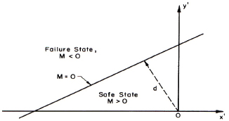
FIGURE C.2 Illustration of safe and failure regions.
In terms of the reduced variates, the limit state equation M = 0 (X – Y = 0) becomes
![]()
From the above figure in the reduced variates, we can clearly distinguish the failure region from the safe region, and distinguish the limit state equation (or failure surface) that separates the two regions. On that basis, the distance, d, from the failure surface to the origin, o, is a measure of safety or reliability and in fact is the safety index β. That distance is (from analytic geometry)
![]()
and thus the probability of failure is
![]()


