
4
Emulation, Reduced-Order Modeling, and Forward Propagation
Computational models simulate a wide variety of detailed physical processes, such as turbulent fluid flow, subsurface hydrology and contaminant transport, hydrodynamics, and also multiphysics, as found in applications such as nuclear reactor analysis and climate modeling, to name only a few examples. The frequently high computational cost of running such models makes their assessment and exploration challenging. Indeed, continually exercising the simulator to carry out tasks such as sensitivity analysis, uncertainty analysis, and parameter estimation is often infeasible. The analyst is instead left to achieve his or her goals with only a limited number of calls to the computational model or with the use of a different model altogether. In this chapter, methods for computer model emulation and sensitivity analysis are discussed.
Two types of emulation settings, designed to solve different, but related, problems, must be distinguished. The first type attempts to approximate the dependence of the computer model outputs on the inputs. In this case, the uncertainty comes from not having observed the full range of model outputs or from the fact that another model is used in place of the costly computational model of interest. These emulators include regression models, Gaussian process (GP) interpolators, and Lagrangian interpolations of the model output, as well as reduced-order models.
The second type of emulation problem—discussed in Section 4.2—is similar, with the additional considerations that the input parameters are now themselves uncertain. So, the aim is to emulate the distribution of outputs, or a feature thereof, under a prespecified distribution of inputs. Statistical sampling of various types (e.g., Monte Carlo sampling) can be an effective tool for mapping uncertainty in input parameters into uncertainty in output parameters (McKay et al., 1979). In its most fundamental form, sampling does not retain the functional dependence of output on input, but rather produces quantities that have been averaged simultaneously over all input parameters. Alternatively, approaches such as polynomial chaos attempt to leverage mathematical structure to achieve more efficient estimates of quantities of interest (QOIs). Indeed, polynomial chaos expansions can lead to a more tractable representation of the uncertainty of the QOIs, which can then be explored using mathematical or computational means.
Finally, a few details should be noted before proceeding. The methods discussed—such as emulation, reduced-order modeling, and polynomial chaos expansions—use output produced from ensembles of simulations carried out at different input settings to capture the behavior of the computational model, the aim being to maximize the amount of information available for the uncertainty quantification (UQ) study given a limited computational budget. The term emulator is most often used to describe the first type of emulation problem and is the terminology adopted hereafter. Furthermore, unless otherwise indicated, the computational models are assumed to be deterministic. That is, code runs repeated at the same input settings will yield the same outputs.
4.1 APPROXIMATING THE COMPUTATIONAL MODEL
Representing the input/output relationships in a model with a statistical surrogate (or emulator) and using a reduced-order model are two broad methods effectively used to reduce the computational cost of model exploration. For instance, a reduced-order model (Section 4.1.2) or an emulator (Section 4.1.1) can be used to stand in place of the computer model when a sensitivity analysis is being conducted or uncertainty is propagating across the computer model (see Section 4.2 and the example on electromagnetic interference phenomena in Section 4.5). Of course, as with any approximation, there is a reduction in the accuracy of the estimates obtained, and the trade-off between accuracy and cost needs to be considered by the analyst.
4.1.1 Computer Model Emulation
In settings in which the simulation model is computationally expensive, an emulator can be used in its place. The computer model is generally viewed as a black box, and constructing the emulator can be thought of as a type of response-surface modeling exercise (e.g., Box and Draper, 2007). That is, the aim is to establish an approximation to the input-output map of the model using a limited number of calls of the simulator.
Many possible parametric and nonparametric regression techniques can provide good approximations to the computer-model response surface. For example, there are those that interpolate between model runs such as GP models (Sacks et al., 1989; Gramacy and Lee, 2008) or Lagrange interpolants (e.g., see Lin et al., 2010). Approaches that do not interpolate the simulations, but which have been used to stand in place of the computer models, include polynomial regression (Box and Draper, 2007), multivariate adaptive regression splines (Jin et al., 2000), projection pursuit (see Ben-Ari and Steinberg, 2007, for a comparison with several methods), radial basis functions (Floater and Iske, 1996), support vector machines (Clarke et al., 2003), and neural networks (Hayken, 1998), to name only a few. When the simulator has a stochastic or noisy response (Iooss and Ribatet, 2007), the situation is similar to the sampling of noisy physical systems in which random error is included in the statistical model, though the variability is likely to also depend on the inputs. In this case, any of the above models can be specified so that the randomness in the simulator response is accounted for in the emulation of the simulator.
Some care must be taken when emulating deterministic computer models if one is interested in representing the uncertainty (e.g., a standard deviation or a prediction interval) in predictions at unsampled inputs. To deal with the difference from the usual noisy settings, Sacks et al. (1989) proposed modeling the response from a computer code as a realization of a GP, thereby providing a basis for UQ (e.g., prediction interval estimation) that most other methods (e.g., polynomial regression) fail to do. A correlated stochastic process model with probability distribution more general than that of the GP could also be used for this interpolation task. A significant benefit of the Gaussian model is the persistence of the tractable Gaussian form following conditioning of the process at the sampled points and the representation of uncertainty at unsampled inputs.
Consider, for example, the behavior of the prediction intervals in Figure 4.1. Figure 4.1(a) shows a GP fit to deterministic computer-model output, and Figure 4.1(b) shows the same data fit using ordinary least squares regression with the set of Legendre polynomials. Both representations emulate the computer model output fairly well, but the GP has some obvious advantages. Notice that the fitted GP model passes through the observed points, thereby perfectly representing the deterministic computational model at the sampled inputs. In addition, the prediction uncertainty disappears entirely at sites for which simulation runs have been conducted (the prediction is the simulated response). Furthermore, the resulting prediction intervals reflect the uncertainty one would expect from a deterministic computer model—zero predictive uncertainty at the observed input points, small predictive uncertainty close to these points, and larger uncertainty farther away from the observed input points.
In spite of the aforementioned advantages, GP and related models do have shortcomings. For example, they are challenging to implement for large ensemble sizes. Many response-surface methods (e.g., polynomial regression or multivariate adaptive regression splines) can handle much larger sample sizes than the GP can and are computationally faster. Accordingly, adapting these approaches so that they can have the same sort of inferential advantages, as shown in Figure 4.1, as those of the GP in the deterministic setting is a topic of ongoing and future research.
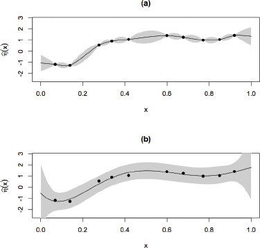
FIGURE 4.1 Two prediction intervals fit to a deterministic computer model: (a) Gaussian process and (b) ordinary least squares regression with Legendre polynomials.
In the coming years, as computing resources become faster and more available, emulation will have to make use of very large ensembles over ever-larger input spaces. Existing emulation approaches tend to break down if the ensemble size is too large. To accommodate larger and larger ensemble sizes, new computational schemes that are suitable for high-performance computing architectures will be required for fitting emulators to computer-model output and producing predictions from these emulators.
Finding: Scalable methods do not exist for constructing emulators that reproduce the high-fidelity model results at each of the N training points, accurately capture the uncertainty away from the training points, and effectively exploit salient features of the response surface.
Finally, most of the current technology for fitting response surfaces treats the computational model as a black box, ignoring features such as continuity or monotonicity that might be present in the physical system being modeled. Augmented emulators that incorporate this phenomenology could provide better accuracy away from training points (Morris, 1991). Current approaches that make use of derivative or adjoint information are examples of emulators that include additional information about the phenomena being modeled.
Finding: Many emulators are constructed only with knowledge about values at training points but do not otherwise include knowledge about the phenomena being modeled. Augmented emulators that incorporate this phenomenology could provide better accuracy away from training points.
An alternative to emulating the computational model is to use a reduced-order version of the forward model— which is itself a reduced-order model of reality. There are several approaches to achieve this, with projection-based model-reduction techniques being the most developed. These techniques aim to identify within the state
space a low-dimensional subspace in which the “dominant” dynamics of the system reside (i.e., those dynamics important for accurate representation of input-output behavior). Projecting the system-governing equations onto this low-dimensional subspace yields a reduced-order model. With appropriate formulation of the model reduction problem, the basis and other elements of the projection process can be precomputed in an off-line phase, leading to a reduced-order model that is rapid to evaluate and solve for new parameter values.
The substantial advances in model reduction over the past decade have taken place largely in the context of forward simulation and control applications; however, model reduction has a large potential to accelerate UQ applications. The challenge is to derive a reduced model that (1) yields accurate estimates of the relevant statistics, meaning that in some cases the model may need to well represent the entire parameter space of interest for the UQ task at hand, and (2) is computationally efficient to construct and solve.
Recent years have seen substantial progress in parametric and nonlinear model reduction for large-scale systems. Methods for linear time-invariant systems are by now well established and include the proper orthogonal decomposition (POD) (Berkooz et al., 1993; Holmes et al., 1996; Sirovich, 1987), Krylov-based methods (Feldsmann and Freund, 1995; Gallivan et al., 1994), balanced truncation (Moore, 1981), and reduced-basis methods (Noor and Peters, 1980; Ghanem and Sarkar, 2003). Extensions of these methods to handle nonlinear and parametrically varying problems have played a major role in moving model reduction from forward simulation and control to applications in optimization and UQ.
Several methods have been developed for nonlinear model reduction. One approach is to use the trajectory piecewise-linear scheme, which employs a weighted combination of linear models, obtained by linearizing the nonlinear system at selected points along a state or parameter trajectory (Rewienski and White, 2003). Other approaches propose using a reduced basis or POD model-reduction approach and approximating the nonlinear term through the selective sampling of a subset of the original equations (Bos et al., 2004; Astrid et al., 2008; Barrault et al., 2004; Grepl et al., 2007). For example, in Astrid et al. (2008), the missing-point-estimation approach, based on the theory of “gappy POD” (Everson and Sirovich, 1995), is used to approximate nonlinear terms in the reduced model with selective spatial sampling. The empirical interpolation method (EIM) is used to approximate the nonlinear terms by a linear combination of empirical basis functions for which the coefficients are determined using interpolation (Barrault et al., 2004; Grepl et al., 2007). Recent work has established the discrete empirical interpolation method (DEIM) (Chaturantabut and Sorensen, 2010), which extends the EIM to a more general class of problems. Although these methods have been successful in a range of applications, several challenges remain for nonlinear model reduction. For example, current methods pose limitations on the form of the nonlinear system that can be considered, and problems with nonlocal nonlinearities can be challenging.
For parametric model reduction, several classes of methods have emerged. Each approach handles parametric variation in a different way, although there is a common theme of interpolation among information collected at different parameter values. The EIM and DEIM methods described above can be used to handle some classes of parametrically varying systems. In the circuit community, Krylov-based methods have been extended to include parametric variations, again with a restriction on the form of systems that can be considered (Daniel et al., 2004). Another class of approaches approximates the variation of the projection basis as a function of the parameters (Allen et al., 2004; Weickum et al., 2006). An alternative for expansion of the basis is interpolation among the reduced subspaces (Amsallem et al., 2007)—for example, using interpolation in the space tangent to the Grassmannian manifold of a POD basis constructed at different parameter points—or among the reduced models (Degroote et al., 2010).
Historically, the use of reduced-order models in UQ is not as common as the surrogate modeling methods (e.g., see Section 4.2) that approximate the full inputs-to-observable map. Some recent examples of model reduction for UQ include statistical inverse problems (Lieberman et al., 2010; Galbally et al., 2010), forward propagation of uncertainty for heat conduction (Boyaval et al., 2009), computational fluid dynamics (Bui-Thanh and Wilcox, 2008), and materials (Kouchmeshky and Zabaras, 2010).
Finding: An important area of future work is the use of model reduction for optimization under uncertainty.
4.2 FORWARD PROPAGATION OF INPUT UNCERTAINTY
In many settings, inputs to a computer model are uncertain and therefore can be treated as random variables. Interest then lies in propagating the uncertainty in the input distribution to the output of the deterministic computer model. It is the distribution of the model outputs, or some feature thereof, that is the primary interest of a typical investigation. For example, one may be interested in the 95th percentile of the output distribution or, perhaps, the mean of the output, along with associated uncertainties.
The set of approaches that either treat the computational model as a black box (nonintrusive techniques) or require modifications to the underlying mathematical model (intrusive techniques) is considered here. In addition, the activities are separated into settings in which (1) the number of simulator evaluations is essentially unlimited (e.g., Monte Carlo and polynomial chaos) and (2) only a relatively small number of simulator runs is available (e.g., Gaussian process, polynomial chaos, and quasi-Monte Carlo).
In a most straightforward manner Monte Carlo sampling can be used—where one can sample directly from the input distribution and evaluate the output of the computer model at each input setting. The estimates for the QOI (mean response, confidence intervals, percentiles, and so on) are obtained from the induced empirical distribution function of the model outputs. Generally, Monte Carlo sampling does not depend on the dimension of the input space or on the complexity of the model. This makes Monte Carlo sampling an attractive approach when the forward model is complicated, has many inputs, and is sufficiently fast. However, in many real-world problems, Monte Carlo methods can require thousands of code executions to produce sufficient accuracy. The number of required function evaluations can be significantly reduced by using quasi-Monte Carlo methods (e.g., see Lemieux, 2009). These rely on relatively few input configurations and attempt to mimic the properties of a random sample to estimate features of the output distribution (e.g., Latin hypercube sampling; McKay et al., 1979; Owen, 1997).
Monte Carlo-based approaches are ill-equipped to take advantage of physical or mathematical structure that could otherwise expedite the calculations. In its most fundamental form, sampling does not retain the functional dependence of output on input but rather produces quantities that have been averaged simultaneously over all input parameters. In contradistinction, the polynomial chaos (PC) methodology (Ghanem and Spanos, 1991; Soize and Ghanem, 2004; Najm, 2009; Xiu and Karniadakis, 2002; Xiu, 2010), capitalizes on the mathematical structure provided by the probability measures on input parameters to develop approximation schemes with a priori convergence results inherited from Galerkin projections and spectral approximations common in numerical analysis. The PC methodology has two essential components. A first step involves a description of stochastic functions, variables, or processes with respect to a basis in a suitable vector space. The choice of basis can be adapted to the distribution of the input parameters (e.g., Xiu and Karniadakis, 2002; Soize and Ghanem, 2004). The second step involves computing the coordinates in this representation using functional analysis machinery, such as orthogonal projections and error minimization. These coordinates permit the rapid evaluation of output quantities of interest as well as of the sensitivities (both local and global) of output uncertainty with respect to input uncertainty.
Two procedures have generally pursued the connection to PC approximations: intrusive and nonintrusive. The so-called nonintrusive approach computes the coefficients in the PC decomposition as multidimensional integrals that are approximated by means of sparse quadrature and other numerical integration rules. The intrusive approach, however, synthesizes new equations that govern the behavior of the coefficients in the PC decomposition from the initial governing equations. Intrusive uncertainty propagation approaches involve a reformulation of the forward model, or its adjoint, to directly produce a probabilistic representation of uncertain model outputs induced by input uncertainty. Such approaches include PC methods, as well as extensions of local sensitivity analysis and adjoint methods. In either case, unlike the first type of emulators described in Section 4.1.1, this class of emulator aims to directly map uncertainty of model input to uncertainty of model output.
Another strategy is to first construct an emulator of the computer model (see Section 4.1.1) and then propagate the distribution of inputs through the emulator (Oakley and O’Hagan, 2002; Oakley, 2004; Cannamela et al., 2008). Essentially, one treats the emulator as if it were a fast computer model and uses the methods already discussed. In these cases, one must account for the variability in the output distribution induced by the random variable as well as the uncertainty in emulating the computer model (Oakley, 2004). Of course, almost all approaches, outside of straight Monte Carlo, will be faced with the curse of dimensionality. Accounting for this induced variability is
an important direction for future research. Interestingly, if the computer model can be assumed to be a GP with known correlation/variance parameters, the propagation of the uncertainty distribution of the model inputs across the GP (i.e., the response surface approach) and polynomial chaos can be viewed as alternative approaches to the same problem, both giving effective approaches for exploring the uncertainty in QOIs.
Consider the particularly challenging problem described in Section 4.5 in which interest lies in estimating statistics (e.g., mean and standard deviation) for observables in an electromagnetic interference (EMI) application. The solution combines features of polynomial chaos expansions and also of emulation followed by uncertainty propagation (Oakley, 2004). For this application, the computer model outputs behave quasi-chaotically as a function of the input configurations. In such cases, emulators that leverage local information instead of a single global model are often more effective. In this specific case study, the computer model is emulated by a nonintrusively computed polynomial chaos decomposition and uses a robust emulator that attempts to model local features. The approach taken is similar to that of Oakley (2004) insofar as the emulator is first constructed and then the distribution of QOIs is approximated by propagating the distribution of inputs across the emulator.
These methods for propagating the variation of the input distribution to explore the uncertainty in the model output are particularly effective when the QOIs are estimates that are centrally located in the output distribution. However, decision makers are often most interested in rare events (e.g., extreme weather scenarios, or a combination of conditions causing system failure). These cases are located in the tails of the output distribution where exploration is often impractical with the aforementioned methods. This problem is only exacerbated for high-dimensional inputs. An important research direction is the estimating of the probability of rare events in light of complicated models and input distributions. One approach to this problem is to bias the model output toward these rare events and properly account for this biasing. Importance sampling (Shahabuddin, 1994) is another approach.
Finding: Further research is needed to develop methods to identify the input configurations for which a model predicts significant rare events and for assessing their probabilities.
Sensitivity analysis (SA) is concerned with understanding how changes in the computational-model inputs influence the outputs or functions of the outputs. There are several motivations for SA, including the following: enhancing the understanding of a complex model, finding aberrant model behavior, seeking out which inputs have a substantial effect on a particular output, exploring how combinations of inputs interact to affect outputs, seeking out regions of the input space that lead to rapid changes or extreme values in output, and gaining insight as to what additional information will improve the model’s ability to predict. Even when a computational model is not adequate for reproducing physical system behavior, its sensitivities may still be useful for developing inferences about key features of the physical system.
In many cases, the most general and physically accurate computational model takes too long to run, making impractical its use as the main tool for a particular investigation and forcing one to seek a simpler, less computationally demanding model. SA can serve as a first step in constructing an emulator and/or a reduced model of a physical system, capturing the important features in a large-scale computational model while sacrificing complexity to speed up the run time. A perfunctory SA also serves as a simplest first step to characterizing output uncertainty induced by uncertainty in inputs (uncertainty analysis is discussed below in this chapter).
Implicit in SA is an underlying surrogate that permits the efficient mapping of changes in input to changes in output. This surrogate highlights the value of emulators and reduced-order models to SA. A few cases in which the peculiar structure of the surrogates allows the analytical evaluation of key sensitivity quantities have attracted particular attention and served to shape the current practice of SA. Local SA is associated with linearization of the input-output map at some judiciously chosen points. Higher-order Taylor expansions have also been used to enhance the accuracy of these surrogates. Global SA, however, relies on global surrogates that better capture the effects of interactions between random variables. Two particular forms of global surrogates have been pursued in recent years that rely, respectively, on polynomial chaos decompositions and Sobol’s decomposition. These decompositions permit the computation of the sensitivity of output variance with respect to the variances of the individual
input parameters. Given the dominance in current research and practice of these particular interpretations of global and local sensitivity, these global SA methods and local SA methods are detailed in the remainder of this section.
4.3.1 Global Sensitivity Analysis
Global SA seeks to understand a complex function over a broad space of input settings, decomposing this function into a sum of increasingly complex components (see Box 4.1). These components might be estimated directly (Oakley and O’Hagan, 2004), or each of these components can be summarized by a variance measure
Box 4.1
Sobol’s Functional Decomposition of a Complex Model
Sobol decomposition of ![]()
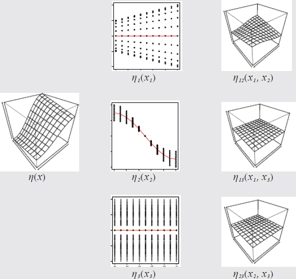
Global sensitivity analysis seeks to decompose a complex model—or function—into a sum of a constant plus main effects plus interactions (Sobol, 1993). Here a three-dimensional function is decomposed into three main effect functions (red lines) η1, η2, and η3 plus three two-way interaction functions η12, η13, and η23 plus a single three-way interaction (not shown). Global sensitivity analysis seeks to estimate these component functions or variance measures of these component functions. See Saltelli et al. (2000) or Oakley and O’Hagan (2004) for examples.
estimated using one of a variety of techniques: Monte Carlo (MC) (Kleijnen and Helton, 1999); regression (Helton and Davis, 2000); analysis of variance (Moore and McKay, 2002); Fourier methods (Sobol, 1993; Saltelli et al., 2000); or GP or other response-surface models (Oakley and O’Hagan, 2004; Marzouk and Najm, 2009). Each of these approaches requires an ensemble of forward model runs to be carried out over a specified set of input settings.
The number of computational-model runs required will depend on the complexity of the forward model over the input space and the dimension of the input space, as well as the estimation method. A key challenge for global SA—indeed, for much of VVUQ—is to carry out such analyses with limited computational resources. The various estimation methods deal with this issue in one way or another. For example, MC methods, while generally requiring many model runs to gain reasonable accuracy, can handle high-dimensional input spaces and arbitrary complexity in the computational model. In contrast, response-surface-based approaches, such as GP, may use an ensemble consisting of very few model runs, but they typically require smoothness and sparsity in the model response (i.e., the response surface depends on only a small set of the inputs). Box 4.1 describes global sensitivity using Sobol decompositions—although these are not the only sensitivity measures. For example, one may be interested in the sensitivity of quantities such as the probability of exceedance (the probability that a QOI will exceed some quantity). In this case, other approaches to global sensitivity must be used.
Finding: In cases where a large-scale computational model is built up from a hierarchy of submodels, there is opportunity to develop efficient SA approaches that leverage this hierarchical construction, taking advantage of separate sensitivity analyses on these submodels. Exactly how to aggregate these separate sensitivity anslyses to give accurate sensitivities on the larger-scale model outputs remains an open problem.
4.3.2 Local Sensitivity Analysis
Local sensitivity analysis is based on the partial derivatives of the forward model with respect to the inputs, evaluated at a nominal input setting. Hence, this sort of SA makes sense only for differentiable outputs. The partial derivatives of the forward model, perhaps scaled, can serve as some indication of how model output responds to input changes. First-order sensitivities—the gradient of an output of interest with respect to inputs—are most commonly used, although second-order sensitivities incorporating partial or full Hessian information can be obtained in some settings. Even higher-order sensitivities have been pursued, albeit with increasing difficulty (emerging tensor methods may make third-order sensitivities more feasible).
Local sensitivities give limited information about forward-model behavior in the neighborhood of the nominal input setting, providing some information about the input-output response of the forward model. Local sensitivity, or derivative information, is more commonly used for optimization (Finsterle, 2006; Flath et al., 2011) in inverse problems (see Section 4.4) or local approximation of the forward model in nonlinear regression problems (Seber and Wild, 2003). In these cases, it is the sensitivity of an objective function, likelihood, or posterior density with respect to the model inputs that is required.
There are two approaches to obtaining local sensitivities: a black box approach and an intrusive approach. In the black box approach, the underlying mathematical or computational model is regarded as being inaccessible, as might be the case with an older, established, or poorly documented code. By contrast, the intrusive approach presumes that the model is accessible, whether because it is sufficiently well documented and modular, or because it is amenable to the retrofitting of local sensitivity capabilities, or because it was developed with local sensitivities in mind.
There are limited options for incorporating local sensitivities into a black box forward code. The classical approach is finite differences. However, this approach can provide highly inaccurate gradient information, particularly when the underlying forward model is highly nonlinear, and “solving” the forward problem amounts to being content with reducing the residual by several orders of magnitude. Moreover, the cost of finite differencing grows linearly with the number of inputs.
An alternative approach is provided by automatic differentiation (AD), sometimes known as algorithmic differentiation. Assuming that one has access to source code, AD is able to produce sensitivity information directly from the source code by exploiting the fact that a code is written from a series of elementary operations, whose known derivatives can be chained together to provide exact sensitivity information. This approach avoids the
numerical difficulties of finite differencing. Furthermore, the so-called reverse mode of AD can be employed to generate gradient information at a cost that is independent (to leading order) of the number of inputs. However, the basic difficulty with AD methods is that they differentiate the code rather than the underlying mathematical model. For example, while the sensitivity equations are linear, AD differentiates through the nonlinear solver; and while sensitivity equations share the same operator, AD repeatedly differentiates through the preconditioner. This also means that artifacts of the discretization (e.g., adaptive mesh refinement) are differentiated. Additionally, when the code is large and complex, current AD tools will often break down. Still, when they do work, and when the intrusive methods described below are not feasible because of time constraints or lack of modularity of the forward code, AD can be a viable approach.
If one has access to the underlying forward model, or if one is developing a local sensitivity capability from scratch, one can overcome many of the difficulties outlined above by using an intrusive method. These methods differentiate the mathematical model underlying the code. This can be done at the continuum level, yielding mathematical derivatives that can then be discretized to produce numerical derivatives. Alternatively, the discretized model may be directly differentiated. These two approaches do not always result in the same derivatives, though often (e.g., with Galerkin discretization) they do. The advantage of differentiating the underlying mathematical model is that one can exploit the model structure. The equations that govern the derivatives of the state variables with respect to each parameter—the so-called sensitivity equations—are linear, even when the forward problem is nonlinear, and they are characterized by the same coefficient matrix (or operator) for each input. This matrix is the Jacobian of the forward model, and thus Newton-based forward solvers can be repurposed to solve the sensitivity equations. Because each right-hand side corresponds to the derivative of the model residual with respect to each parameter, the construction of the preconditioner can be amortized over all of the inputs.
Still, solving the sensitivity equations may prove too costly when there are large numbers of inputs. An alternative to the sensitivity equation approach is the so-called adjoint approach, in which an adjoint equation1 is solved for each output of interest, and the resulting adjoint solution is used to construct the gradient (analogs exist for higher derivatives). This adjoint equation is, like the sensitivity equation, always linear in the adjoint variable, and its right-hand side corresponds to the derivative of the output with respect to the state. Its operator is the adjoint (or transpose) of the linearized forward model, and so here again preconditioner construction can be amortized, in this case over the outputs of interest. When the number of outputs is substantially less than the number of input parameters, the adjoint approach can result in substantial savings. By postponing discretization until after derivatives have been derived (through variational means), one can avoid differentiating artifacts of the discretization (e.g., subgrid-scale models, flux limiters).
Even first derivatives can greatly extend one’s ability to explore the forward model’s behavior in the service of UQ, especially when the input dimension is large. If derivative information can be calculated for the cost of only an additional model run, as is often the case with adjoint models, then tasks such as global SA, solving inverse problems, and sampling from a high-dimensional posterior distribution can be carried out with far less computational effort, making currently intractable problems tractable.
Generalizing adjoint methods to better tackle difficult computational problems such as multiphysics applications, operator splitting, and nondifferentiable solution features (such as shocks) would extend the universe of problems for which derivative information can be efficiently computed. At the same time, developing and extending UQ methods to take better advantage of derivative information will broaden the universe of problems for which computationally intensive UQ can be carried out. Current examples of UQ methods applicable to large-scale computational models that take advantage of derivative information include normal linear approximations for inverse problems (Cacuci et al., 2005), response surface methods (Mitchell et al., 1994), and Markov chain MC sampling techniques for Bayesian inverse problems (Neal, 1993; Girolami and Calderhead, 2011).
Finding: There is potential for significant benefit from research and development in the compound area of (1) extracting derivatives and other features from large-scale computational models and (2) developing UQ methods that efficiently use this information.
_____________________
1 A discussion is given in Marchuk (1995).
4.4 CHOOSING INPUT SETTINGS FOR ENSEMBLES OF COMPUTER RUNS
An important decision in an exploration of the simulation model is the choice of simulation runs (i.e., experimental design) to perform. Ultimately, the task at hand is to provide an estimate of some feature of the computer model response as efficiently as possible. As one would expect, the optimal set of model evaluations is related to the specific aims of the experimenter.
For physical experiments, there are three broad principles for experimental design: randomization, replication, and blocking.2 For deterministic computer experiments, these issues do not apply—replication, for example, is just wasted effort. In the absence of prior knowledge of the shape of the response surface, however, a simple rule of thumb worth following is that the design points should be spread out to explore as much of the input region as possible.
Current practice for the design of computer experiments identifies strategies for a variety of objectives. If the goal is to identify the active factors governing the system response, one-at-a-time designs3 are commonly used (Morris, 1991). For computer-model emulation, space-filling designs (Johnson and Schneiderman, 1991), and Latin hypercube designs (McKay et al., 1979) and variants thereof (Tang, 1993; Lin et al., 2010) are good choices. The designs used for building emulators are often motivated by space-filling and projection properties that are important for quasi-MC studies (Lemieux, 2009). In studies in which the goal is to estimate a feature of the computer-model response surface, such as a global maximum or level sets, sequential designs have proven effective (Ranjan et al., 2008). In these cases, one is usually attempting to select new simulator trials that aim to optimally improve the estimate of the feature of interest rather than the estimate of the entire response surface. For SA, common design strategies include fractional factorial and response-surface designs (Box and Draper, 2007), as well as Morris’s one-at-a-time designs and other screening designs (e.g., Saltelli and Sobol, 1995). The use of adaptive strategies for the larger V&V problem is discussed in Chapter 5.
4.5 ELECTROMAGNETIC INTERFERENCE IN A TIRE PRESSURE SENSOR: CASE STUDY
The proper functioning of electronic communication, navigation, and sensing systems often is disturbed, upset, or blocked altogether by electromagnetic interference (EMI)—viz, natural or man-made signals that are foreign to the systems’ normal mode of operation. Natural EMI sources include atmospheric charge/discharge phenomena such as lightning and precipitation static. Man-made EMI can be intentional—arising from jamming or electronic warfare—or unintentional, resulting from spurious electromagnetic emissions originating from other electronic systems.
To guard mission-critical electronic systems against interference and ensure system interoperability and compatibility, engineers employ a variety of electromagnetic shielding and layout strategies to prevent spurious radiation from penetrating into, or escaping from, the system. This practice is especially relevant for consumer electronics subject to regulation by the Federal Communications Commission. In developing EMI mitigation strategies, it is important to recognize that many EMI phenomena are stochastic in nature. The degree to which EMI affects a system’s performance is influenced by its electromagnetic environment, e.g., its mounting platform and proximity to natural or man-made sources of radiation. Unfortunately, a system’s electromagnetic environment oftentimes is ill-characterized at the time of design. The uncertainty in the effect of EMI on a system’s performance is further exacerbated by variability in its electrical and material component values and geometric dimensions.
Although the EMI compliance of a system prior to deployment or mass production always is verified experimentally, engineers increasingly rely on modeling and simulation to reduce costs associated with the building and
_____________________
2 Blocking is the arrangement of experimental units into groups.
3 One-at-a-time designs are designs that vary one variable at a time.
testing of prototypes early in the design process. EMI phenomena are governed by Maxwell’s equations. These equations have astonishing predictive power, and their reach extends far beyond EMI analysis. Indeed, Maxwell’s equations form the foundation of electrodynamics and classical optics and the underpinnings of many electrical, computer, and communication technologies. Fueled by advances in both algorithms and computer hardware, Maxwell equation solvers have become indispensable in scientific and engineering disciplines ranging from remote sensing and biomedical imaging to antenna and circuit design, to name but a few.
The application of VVUQ concepts to the statistical characterization of EMI phenomena described below leverages an integral equation-based Maxwell equation solver. The solver accepts as input a computer-aided design (CAD) description of a system’s geometry along with its external excitation, and returns a finite-element approximation of the electrical currents on the system’s conducting surfaces, shielding enclosures, printed circuit boards, wires/cables, and dielectric (plastic) volumes (Bagci et al., 2007). To enable the simulation of EMI phenomena on large- and multiscale computing platforms, the solver executes in parallel and leverages fast and highly accurate O[N log(N)] convolution methods, causing its computational cost to scale roughly linearly with the number of unknowns in the finite-element expansion. To facilitate the characterization of real-world EMI phenomena, the solver interfaces with a Simulation Program with Integrated Circuit Emphasis (SPICE)4-based circuit solver that computes node voltages on lumped element circuits that model electrically small components. Finally, to allow for the characterization of a “system of systems,” the Maxwell equation solver interfaces with a cable solver that computes transmission-line voltages and currents on transmission lines interconnecting electronic (sub)systems (Figure 4.2).
The application of this hybrid analysis framework to the statistical characterization of EMI phenomena in real-world electronic systems is illustrated by means of a tire pressure monitoring (TPM) system (Figure 4.3). TPM systems monitor the air pressure of vehicle tires and warn drivers when a tire is under-inflated. The most widely used TPM system uses a small battery-operated sensor-transponder mounted on a car’s tire rim just behind the valve stem. The sensor-transponder transmits information on the tire pressure and temperature to a central TPM
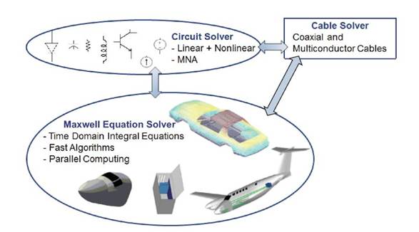
FIGURE 4.2. Hybrid electromagnetic interference analysis framework composed of Maxwell equation, circuit, and cable solvers.
_____________________
4 SPICE is a general-purpose open-source analog electronic circuit simulator.
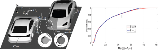
FIGURE 4.3 (Left) Two cars with tire pressure monitoring (TPM) systems mounted on their front-passenger-side wheel rims. (Right) Comparison of cumulative distribution functions of the TPM received signal on one car, without (k = 1) and with (k = 2) the second car present
receiver mounted on the body of the car. In this case study, the strength of the received signal when the system is subject to EMI originating from another nearby car using the same system is characterized. The received signal depends on the relative position of the two cars, described by seven parameters: the rotation and steering angles of the wheels of both cars carrying the TPM transponders, the height of the car bodies with respect to their wheel base, and the relative position of the cars with respect to each other.
In principle, statistics pertaining to the strength of the received signal can be deduced by an MC method, namely by repeatedly executing the Maxwell equation solver for many realizations of the random parameters sampled with respect to their probability distribution functions, which here are assumed to be uniform. Unfortunately, while such an MC method is straightforward to implement, for the problem at hand it requires hundreds of thousands of deterministic code executions to converge. The slow convergence of the MC method combined with the fact that execution of the deterministic Maxwell equation solver for the TPM problem requires roughly 1 hour of central processing unit (CPU) time all but rules out its direct application.
To avoid the pitfalls associated with the direct application of MC, an emulator (or surrogate model) for the strength of the received TPM signal (the QOI) as a function of the seven input parameters was constructed for this study. The emulator provides an accurate approximation of the received signal for all combinations of the parameters, yet can be evaluated in a fraction of the time required for executing the Maxwell equation solver. The emulator thus enables the cost-effective, albeit indirect, application of MC to the statistical characterization of the received TPM signal. In this case study, the emulator was constructed by means of a multielement stochastic collocation (ME-SC) technique that leverages generalized polynomial chaos (gPC) expansions to represent the received signal (Xiu, 2007; Agarwal and Aluru, 2009).
The ME-SC method is an extension of the basic SC method, which approximates a selected QOI (in this case the received TPM signal) by polynomials spanning the entire input parameter space. The SC method constructs these polynomials by calling a deterministic simulator—here a Maxwell solver—to evaluate the QOI for combinations of random inputs specified by collocation points in the seven-dimensional input space. Unfortunately, basic SC methods oftentimes become impractical and inaccurate for outputs that vary rapidly or nonsmoothly with changes in the input parameters, because their representation calls for high-order polynomials. Such is the case in EMI analysis, in which voltages across system pins and currents on circuit traces and the received TPM signal strength, behave rapidly and sometimes quasi-chaotically in the input space. Fortunately, extensions to SC methods have been developed that remain efficient and accurate for modeled outputs with nonsmooth and/or discontinuous
dependencies on the inputs. The ME-SC method is one of them. It achieves its efficiency and accuracy by adaptively dividing the input space into subdomains based on the decay rates of the outputs’ local variances and constructing separate polynomial approximations for each subdomain (Agarwal and Aluru, 2009).
The use of emulators adds uncertainty to the process of statistically characterizing EMI phenomena for which it is often difficult to account. Indeed, the construction of the emulator by means of ME-PC methods involves a greedy search for a sparse basis for the random inputs. When applied to complex, real-world problems, this search is not guaranteed to converge or to yield an accurate representation of the QOI. In the context of EMI analysis, emulator techniques often are applied to simple toy problems that qualitatively relate to the real-world problem at hand, yet allow for an exhaustive canvasing of input space. If and when the method performs well on the toy problem, it is then applied to more complex, real-world scenarios, often without looking back.
The ME-SC emulator models the signal strength in the TPM receiver in one car radiated by simultaneously active sensor-transponders in both cars. Construction of the ME-SC emulator required 545 calls of the Maxwell equation solver, a very small fraction of the number of calls required in the direct application of MC. The relative accuracy of the ME-SC emulator with respect to the signal strength predicted by the Maxwell equation solver was below 0.1 percent for each of the 545 system configurations in the seven-dimensional input space. The cost of applying MC to the emulator is negligible compared to that of a single call to the Maxwell equation solver. Figure 4.3(right) shows the cumulative distribution function (cdf) of the received signal (QOI) and compares it to the cdf produced with only one car present. The presence of the second car does not substantially alter the cdf for small values of the received signal. It does substantially increase the maximum possible received signal, albeit not enough to cause system malfunction.
Agarwal, N., and N. Aluru. 2009. A Domain Adaptive Stochastic Collocation Approach for Analysis of MEMS Under Uncertainties. Journal of Computational Physics 228:7662-7688.
Allen, M., G. Weickum, and K. Maute. 2004. Application of Reduced-Order Models for the Stochastic Design Optimization of Dynamic Systems. Pp. 1-20 in Proceedings of the 10th AIAA/ISSMO Multidisciplinary Optimization Conference. August 30-September 1, 2004. Albany, N.Y.
Amsallem, D., C. Farhat, and T. Lieu. 2007. High-Order Interpolation of Reduced-Order Models for Near Real-Time Aeroelastic Prediction. Paper IF-081:18-20. International Forum on Aeroelasticity and Structural Dynamics. Stockholm, Sweden.
Astrid, P., S. Weiland, K. Willcox, and T. Backx. 2008. Missing Point Estimation in Models Described by Proper Orthogonal Decomposition. IEEE Transactions on Automatic Control 53(10):2237-2251.
Bagci, H., A.E. Yilmaz, J.M. Jin, and E. Michielssen. 2007. Fast and Rigorous Analysis of EMC/EMI Phenomena on Electrically Large and Complex Cable-Loaded Structures. IEEE Transactions on Electromagnetic Compatibility 49:361-381.
Barrault, M., Y. Maday, N.C. Nguyen, and A.T. Patera. 2004. An “Empirical Interpolation” Method: Application to Efficient Reduced-Basis Discretization of Partial Differential Equations. Comptes Rendus Mathematique 339(9):667-672.
Ben-Ari, E.N., and D.M. Steinberg. 2007. Modeling Data from Computer Experiments: An Empirical Comparison of Kriging with MARS and Projection Pursuit Regression. Quality Engineering 19:327-338.
Berkooz, G., P. Holmes, and J.L. Lumley. 1993. The Proper Orthogonal Decomposition in the Analysis of Turbulent Flows. Annual Review of Fluid Dynamics 25:539-575.
Bos, R., X. Bombois, and P. Van den Hof. 2004. Accelerating Large-Scale Non-Linear Models for Monitoring and Control Using Spatial and Temporal Correlations. Proceedings of the American Control Conference 4:3705-3710.
Box, G.E.P., and N.R. Draper. 2007. Response Surfaces, Mixtures, and Ridge Analysis. Wiley Series in Probability and Statistics, Vol. 527. Hoboken, N.J.: Wiley.
Boyaval, S., C. LeBris, Y. Maday, N.C. Nguyen, and A.T. Patera. 2009. A Reduced Basis Approach for Variational Problems with Stochastic Parameters: Application to Heat Conduction with Variable Robin Coefficient. Computer Methods in Applied Mechanics and Engineering 198:3187-3206.
Bui-Thanh, T., and K. Willcox. 2008. Parametric Reduced-Order Models for Probabilistic Analysis of Unsteady Aerodynamic Applications. AIAA Journal 46 (10):2520-2529.
Cacuci, D.C., M. Ionescu-Bujor, and I.M. Navon. 2005. Sensitivity and Uncertainty Analysis: Applications to Large-Scale Systems, Vol. 2. Boca Raton, Fla.: CRC Press.
Cannamela, C., J. Garnier, and B. Iooss. 2008. Controlled Stratification for Quantile Estimation. Annals of Applied Statistics 2(4):1554-1580.
Chaturantabut, S., and D.C. Sorensen. 2010. Nonlinear Model Reduction via Discrete Empirical Interpolation. SIAM Journal on Scientific Computing 32(5):2737-2764.
Clarke, S.M., M.D. Zaeh, and J.H. Griebsch. 2003. Predicting Haptic Data with Support Vector Regression for Telepresence Applications. Pp. 572-578 in Design and Application of Hybrid Intelligent Systems. Amsterdam, Netherlands: IOS Press.
Daniel, L., O.C. Siong, L.S. Chay, K.H. Lee, and J. White. 2004. A Multiparameter Moment-Matching Model-Reduction Approach for Generating Geometrically Parameterized Interconnect Performance Models. IEEE Transactions on Computer-Aided Design of Integrated Circuits and Systems 23(5):678-693.
Degroote, J., J. Vierendeels, and K. Wilcox. 2010. Interpolation Among Reduced-Order Matrices to Obtain Parametrized Models for Design, Optimization and Probabilistic Analysis. International Journal for Numerical Methods in Fluids 63(2):207-230.
Everson, R., and L. Sirovich. 1995. Karhunen-Loève Procedure for Gappy Data. Journal of the Optical Society of America 12(8):1657-1664.
Feldman, P., and R.W. Freund. 1995. Efficient Linear Circuit Analysis by Pade Appoximation via the Lanczos Process. IEEE Transactions on Computer-Aided Design of Integrated Circuits 14(5):639-649.
Finsterle, S. 2006. Demonstration of Optimization Techniques for Groundwater Plume Remediation Using Itough2. Environmental Modeling and Software 21(5):665-680.
Flath, H.P., L.C. Filcox, V. Akcelik, J. Hill, B. Van Bloeman Waanders, and O. Glattas. 2011. Fast Algorithms for Bayesian Uncertainty Quantification in Large-Scale Linear Inverse Problems Based on Low-Rank Partial Hessian Approximations. SIAM Journal on Scientific Computing 33(1):407-432.
Floater, M.S., and A. Iske. 1996. Multistep Scattered Data Interpolation Using Compactly Supported Radial Basis Functions. Journal of Computational and Applied Mathematics 73(1-2):65-78.
Galbally, D., K. Fidkowski, K. Willcox, and O. Ghattas. 2010. Non-Linear Model Reduction for Uncertainty Quantification in Large-Scale Inverse Problems. International Journal for Numerical Methods in Engineering 81:1581-1608.
Gallivan, K.E., E. Grimme, and P. Van Dooren. 1994. Pade Approximations of Large-Scale Dynamic Systems with Lanczos Methods. Decision and Control: Proceedings of the 33rd IEEE Conference 1:443-448.
Ghanem, R., and A. Sarkar. 2003. Reduced Models for the Medium-Frequency Dynamics of Stochastic Systems. Journal of the Acoustical Society of America 113(2):834-846.
Ghanem, R., and P. Spanos. 1991. A Spectral Stochastic Finite Element Formulation for Reliability Analysis. Journal of Engineering Mechanics, ASCE 117(10):2351-2372.
Girolami, M., and B. Calderhead. 2011. Reimann Manifold Langevin and Hamiltonian Monte Carlo Methods. Journal of the Royal Society: Series B (Statistical Methodology) 73(2):123-214.
Gramacy, R.B., and H.K.H. Lee. 2008. Bayesian Treed Gaussian Process Models with an Application to Computer Modeling. Journal of the American Statistical Association 103(483):1119-1130.
Grepl, M.A., Y. Maday, N.C. Nguyen, and A.T. Patera. 2007. Efficient Reduced-Basis Treatment of Nonaffine and Nonlinear Partial Differential Equations. ESAIM-Mathematical Modeling and Numerical Analysis (M2AN) 41:575-605.
Hayken, S. 1998. Neural Networks: A Comprehensive Foundation. Upper Saddle River, N.J.: Prentice Hall.
Helton, J.C., and F.J. Davis. 2000. Sampling-Based Methods for Uncertainty and Sensitivity Analysis. Albuquerque, N.Mex.: Sandia National Laboratories.
Holmes, P., J.L. Lumley, and G. Berkooz. 1996. Turbulence, Coherent Structures, Dynamical Systems, and Symmetry. Cambridge, U.K.: Cambridge University Press.
Iooss, B., and M. Ribatet. 2007. Global Sensitivity Analysis of Stochastic Computer Models with Generalized Additive Models. Technometrics.
Jin, R., W. Chen, and T.W. Simpson. 2000. Comparative Studies of Metamodeling Techniques. European Journal of Operations Research 138:132-154.
Johnson, B., and B. Schneiderman. 1991. Tree-Maps: A Space-Filling Approach to the Visualization of Hierarchical Information Structures. Pp. 284-291 in Proceedings of IEEE Conference on Visualization.
Kleijnen, J.P.C., and J.C. Helton. 1999. Statistical Analyses of Scatterplots to Identify Important Factors in Large-Scale Simulations. 1: Review and Comparison of Techniques. Reliability Engineering and System Safety 65:147-185.
Kouchmeshky, B., and N. Zabaras. 2010. Microstructure Model Reduction and Uncertainty Quantification in Multiscale Deformation Process. Computational Materials Science 48(2):213-227.
Lemieux, C. 2009. Monte Carlo and Quasi-Monte Carlo Sampling. Springer Series in Statistics. New York: Springer.
Lieberman, C., K. Wilcox, and O. Ghattas. 2010. Parameter and State Model Reduction for Large-Scale Statistical Inverse Problems. SIAM Journal on Scientific Computing 32(5):2523-2542.
Lin, C.D., D. Bingham, R.R. Sitter, and B. Tang. 2010. A New and Flexible Method for Constructing Designs for Computer Experiments. Annals of Statistics 38(3):1460-1477.
Marchuk, D.I. 1995. Adjoint Equations and Analysis of Complex Systems. Dordrecht, The Netherlands: Kluwer Academic Publishers.
Marzouk, Y.M., and H.N. Najm. 2009. Dimensionality Reduction and Polynomial Chaos Acceleration of Bayesian Inference in Inverse Problems. Journal of Computational Physics 228:1862-1902.
McKay, M.D., R.J. Beckman, and W.J. Conover. 1979. A Comparison of Three Methods for Selecting Values of Input Variables in the Analysis of Output from a Computer Code. Technometrics 21(2):239-245.
Mitchell, T.J., M.D. Morris, and D. Ylvisaker. 1994. Asymptotically Optimum Experimental Designs for Prediction of Deterministic Functions Given Derivative Information. Journal of Statistical Planning and Inference 41:377-389.
Moore, L.M. 1981. Principle Component Analysis in Linear Systems: Controllability, Observability, and Model Reduction. IEEE Transactions on Automatic Control 26(1):17-31.
Moore, L.M., and M.D. McKay. 2002. Orthogonal Arrays for Computer Experiments to Assess Important Inputs. D.W. Scott (Ed.). Pp. 546-551 in Proceedings of PSAM6, 6th International Conference on Probabilistic Safety Assessment and Management.
Morris, M. 1991. Factorial Sampling Plans for Preliminary Computational Experiments. Technometrics 33(2):161-174.
Najm, H.N. 2009. Uncertainty Quantification and Polynomial Chaos Techniques in Computational Fluid Dynamics. Annual Review of Fluid Mechanics 41:35-52.
Neal, R.M. 1993. Probabilistic Inference Using Markov Chain Monte Carlo Methods. CRG-TR-93-1. Toronto, Canada: Department of Computer Science, University of Toronto.
Noor, A.K., and J.M. Peters. 1980. Nonlinear Analysis via Global-Local Mixed Finite Element Approach. International Journal for Numerical Methods in Engineering 15(9):1363-1380.
Oakley, J. 2004. Estimating Percentiles of Uncertain Computer Code Outputs. Journal of the Royal Statistical Society: Series C (Applied Statistics) 53(1):83-93.
Oakley, J., and A. O’Hagan. 2002. Bayesian Inference for the Uncertainty Distribution of Computer Model Outputs. Biometrika 89(4):769-784.
Oakley, J., and A. O’Hagan. 2004. Probabilistic Sensitivity Analysis of Complex Models: A Bayesian Approach. Journal of the Royal Statistical Society: Series B (Statistical Methodology) 66(3):751-769.
Owen, A.B. 1997. Monte Carlo Variance of Scrambled Net Quadrature. SIAM Journal on Numerical Analysis 34(5):1884-1910.
Ranjan, P., D. Bingham, and G. Michailidis. 2008. Sequential Experiment Design for Contour Estimation from Complex Computer Codes. Technometrics 50(4):527-541.
Rewienski, M., and J. White. 2003. A Trajectory Piecewise-Linear Approach to Model Order Reduction and Fast Simulation of Nonlinear Circuits and Micromachined Devices. IEEE Transactions on Computer-Aided Design of Integrated Circuits and Systems 22(2):155-170.
Sacks, J., W.J. Welch, T.J. Mitchell, and H.P. Win. 1989. Design and Analysis of Computer Experiments. Statistical Science 4(4):409-423.
Saltelli, A., and I.M. Sobol. 1995. About the Use of Rank Transformation in Sensitivity Analysis of Model Output. Reliability Engineering and System Safety 50(3):225-239.
Saltelli, A., K. Chan, and E.M. Scott. 2000. Sensitivity Analysis. Wiley Series in Probability and Statistics, Vol. 535. Hoboken, N.J.: Wiley.
Seber, G.A.F., and C.J. Wild. 2003. Nonlinear Regression. Hoboken, N.J.: Wiley.
Shahabuddin, P. 1994. Importance Sampling for the Simluation of Highly Reliable Markovian Systems. Management Science 40(3):333-352.
Sirovich, L. 1987. Turbulence and the Dynamics of Coherent Structures. Part I: Coherent Structures. Quarterly Journal of Applied Mathematics XLV(2):561-571.
Sobol, W.T. 1993. Analysis of Variance for “Component Stripping” Decomposition of Multiexponential Curves. Computer Methods and Programs in Biomedicine 39(3-4):243-257.
Soize, C., and R. Ghanem. 2004. Physical Systems with Random Uncertainties: Chaos Representations with Arbitrary Probability Measure. SIAM Journal on Scientific Computing 26(2):395-410.
Tang, B. 1993. Orthogonal Array-Based Latin Hypercubes. Journal of the American Statistical Association 88(424):1392-1397.
Weickum, G., M.S. Eldred, and K. Maute. 2006. Multi-Point Extended Reduced-Order Modeling for Design Optimization and Uncertainty Analysis. Paper AIAA-2006-2145. Proceedings of the 47th AIAA/ASME/ASCE/AHS/ASC Structures, Structural Dynamics, and Materials Conference (2nd AIAA Multidisciplinary Design Optimization Specialist Conference). May 1-4, 2006, Newport, R.I.
Xiu, D. 2007. Efficient Collocational Approach for Parametric Uncertainty Analysis. Communications in Computational Physics 2:293-309.
Xiu, D. 2010. Numerical Methods for Stochastic Computations: A Spectral Method Approach. Princeton, N.J.: Princeton University Press.
Xiu, D., and G.E. Karniadakis. 2002. Modeling Uncertainty in Steady State Diffusion Problems via Generalized Polynomial Chaos. Computer Methods in Applied Mechanics and Engineering 191(43):4927-4943.


