
2
Microwave Fundamentals
The initial surge in microwave technology development was driven by the military needs of the second world war. The tremendous effort that went into development of radar during World War II generated a great body of knowledge on the properties of microwaves and related technologies. Much of this information was documented in a series of volumes edited by Massachusetts Institute of Technology Radiation Laboratory under the supervision of the National Defense Research Committee (MIT, 1948; Ragan, 1948).
A basic understanding of microwaves and their interaction with materials is required to realize the promise, as well as to understand the limitations, of microwave processing. Although there is a broad range of materials that can be processed using microwaves, there are fundamental characteristics and properties that make some materials particularly conducive to microwave processing and others difficult. While an empirical understanding of microwave processing is important in moving developmental processes into production, a more fundamental approach is required for development of optimized process cycles, equipment, and controls. For instance, repeatability of a measurement is challenging in microwave processing since the results can be affected by a myriad of factors, including moisture content, changes in dielectric properties during processing, electromagnetic interference with temperature measurements, sample size and geometry, or placement of the sample within the cavity.
The purpose of this chapter is to discuss, in general terms, how microwaves are generated, introduce the fundamental nature of microwaves, how they interact with materials, and how these interactions generate process heat. The application of these fundamental concepts for design or selection of a practical processing system is discussed in Chapter 3. The unique performance characteristics that arise from the interactions of microwaves and materials and how they may be used to develop application criteria are described in Chapter 4.
The spectrum of electromagnetic waves spans the range from a few cycles per second in the radio band to 1020 cycles per second for gamma rays (Figure 2-1). Microwaves occupy the part of the spectrum from 300 MHz (3 × 10⁸ cycles/s) to 300 GHz (3 × 10¹¹ cycles/s). Typical frequencies for materials processing are 915 MHz, 2.45 GHz, 5.8 GHz, and 24.124 GHz.
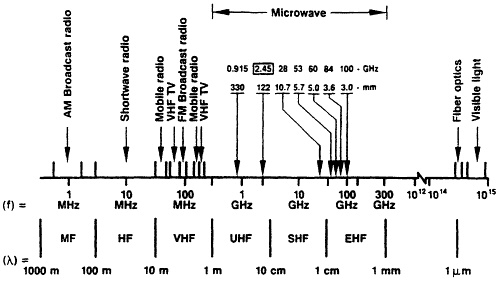
FIGURE 2-1 Electromagnetic spectrum and frequencies used in microwave processing (Sutton, 1993).
MICROWAVE GENERATORS
Major advances in microwave generation and generators occurred in the early 1940s with the invention, rapid development, and deployment of the cavity magnetron on the heels of the earlier (1938) invention of the klystron. What started as "flea powered" curiosities are now capable of generating hundreds of megawatts of power.
The genesis of microwave generator development was the introduction of DeForest's audion tube, the first electron tube amplifier, in 1907. In addition to being developed to be capable of generating megawatts of continuous-wave power (albeit limited in operating frequencies to the region below 1,000 MHz), the audion tube led to the lineage of microwave tubes. Figure 2-2 traces, in time, that beginning and the inventions and developments that followed. The dependence of one tube on the understanding and development of others is illustrated.
A historical discussion of microwave generators would be incomplete without highlighting two major developments. The first involved space charge and the transit time of electron motion within a vacuum, which represented a fundamental limitation to the operating frequency and output power of conventional gridded tubes. When the time of transit became an appreciable part of a microwave frequency cycle, performance degraded, forcing the designer to smaller and smaller sizes to achieve higher frequency. The invention of the kylstron obviated this limitation by utilizing space-charge effects and transit-time effects in a device whose dimensions encompass many wavelengths. A klystron today is capable of peak output power of 100 megawatts at 10 GHz.
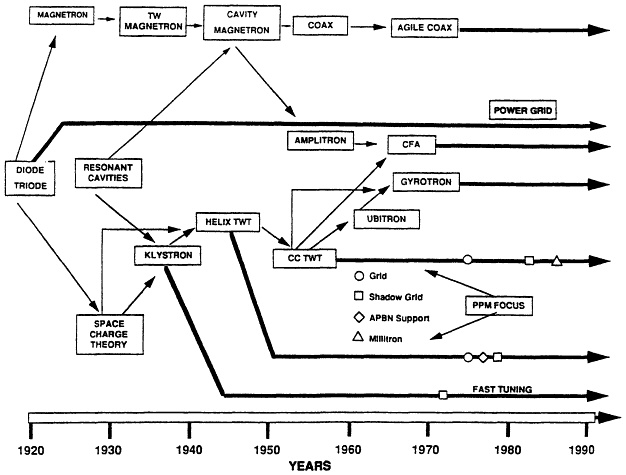
FIGURE 2-2 Microwave Tube Development.
At even higher frequency and higher power levels, limitations associated with voltage and size were encountered. The second major invention occurred in Russia with the realization that the citron relativistic mass change at high voltages could be fundamental to a new type of beam—wave interaction. This led to the development of the gyrotron, later brought to a high state of development in this country. Power/frequency goals of 1 MW continuous wave at 140 GHz are being pursued.
Large performance improvements have been achieved through the application of new materials and processes in microwave generators. For example, the application and ready availability of high thermal conductivity beryllium oxide or boron nitride has allowed signifier improvements in maximum continuous wave power output of traveling wave tubes (from approximately 3 W to 3 kW).
With roots in military radar, today's microwave tubes find applications in medical, scientific, broadcast, communication, and industrial equipment.
CANDIDATE GENERATORS
It is instructive to show device performance range on a power—frequency plot, as in Figure 2-3.
In addition to power and frequency, other performance factors are important to specific applications. Gain, linearity, noise, phase and amplitude stability, coherence, size, weight, and cost must also be considered. Currently available microwave generators include power grid tubes, klystrons, klystrodes (a combination of tetrode power grid tube and klystron), magnetrons, crossed-field amplifiers, traveling wave tubes, and gyrotrons. Those most applicable to materials processing are described.
Table 2-1 shows the most likely candidate tubes, together with a few salient characteristics, including device cost and cost per watt of power generated. The cost of the ancillary equipment such as power conditioning, control circuitry, transmission line, and applicator must be added to the numbers shown. A discussion of cost issues for microwave processing is included in Chapter 4.
Magnetron
At the customary microwave frequencies, the magnetron is the workhorse, the economic product of choice for the generation of "raw" power. These are the tubes used in conventional microwave ovens found in almost every home (with power on the order of a kilowatt in the 2—3 GHz range) and in industrial ovens with output to a megawatt.
Radars employing magnetrons number in the tens of thousands, and household ovens employing the so-called "cooker magnetron" number in the tens of millions. Large quantifies often lead to lower cost, and thus for many microwave heating and processing applications the magnetron is the device of choice, with advantages in size, weight, efficiency, and cost.
The magnetron is the major player in a class of tubes termed "crossed field," so named because the basic interaction depends upon electron motion in electric and magnetic fields that are perpendicular to one another and thus "crossed." In its most familiar embodiment, shown schematically in Figure 2-4, a cylindrical electron emitter, or cathode, is surrounded by a cylindrical structure, or anode, at high potential and capable of supporting microwave fields. Magnets are arranged to supply a magnetic field parallel to the axis and hence perpendicular to the anode cathode electric field.
The interaction of electrons traveling in this crossed field and microwave fields supplied by the anode causes a net energy transfer from the applied DC voltage to the microwave field. The interaction occurs continuously as the electrons traverse the cathode anode region. The magnetron is the most efficient of the microwave tubes, with efficiencies of 90 percent having
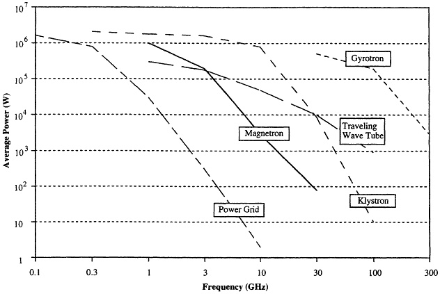
FIGURE 2-3 Power——frequency limits of microwave generators.
been achieved and with 70—80 percent efficiencies common. Figure 2-5 shows the conventional "cooker magnetron." Figure 2-6 is an industrial heating magnetron designed to operate at 2,450 MHz at the 8 kW level.
Power Grid Tubes
At somewhat lower frequencies, power-grid tubes (triodes, tetrodes, etc.) are selected for their lower cost. These can be the same as tubes utilized in AM and FM radio broadcasting and in television. The large user base provides the quantity factor important to economical manufacturing and hence low cost.
The power-grid robe consists of a planar element emitting electrons (cathode) near a parallel planar element receiving electrons (anode) and of an interspersed parallel grid controlling the electron flow. With proper DC voltages applied to the three elements, a microwave signal impressed on the grid results in a much larger (amplified) signal at the anode.
The performance of power-grid robes rages from low-power tubes capable of roughly a kilowatt of output at frequencies of 350 MHz to very-high-power tubes used in fusion research
TABLE 2-1 Microwave Tube Characteristics
|
|
Power KW |
Frequency GHz |
Efficiency % |
Cost $K |
Cost $/Watt |
Special Rqmts. |
|
Magnetron |
|
|
|
|
|
|
|
''Cooker'' |
1 |
2.45 |
60-70 |
0.05 |
0.05 |
|
|
Industrial |
5 to 15 |
2.45 |
60-70 |
3.50 |
0.35 |
|
|
Industrial |
50 |
0.915 |
60-70 |
5.00 |
0.10 |
|
|
Power Grid (Transmitting) |
|
|
|
|
|
|
|
"Low" |
to 10 |
to 3 |
80s |
|
0.1 to .4 |
ex |
|
"Medium" |
to 100 |
to 1 |
80s |
|
0.10 |
ex |
|
"High" |
to 2000 |
to .15 |
80s |
|
0.10 |
ex |
|
Klystron |
|
|
|
|
|
|
|
Example |
500 |
3 |
60s |
350.00 |
0.70 |
s |
|
Example |
250 |
6 |
60s |
200.00 |
0.80 |
s |
|
Example |
250 |
10 |
60s |
375.00 |
1.50 |
s |
|
Klystrode |
|
|
|
|
|
|
|
Example |
30 |
1 |
70s |
18.00 |
0.60 |
s, ex |
|
Example |
60 |
1 |
70s |
36.00 |
0.60 |
s, ex |
|
Example |
500 |
1 |
70s |
Dev. |
~ 1 |
s, ex |
|
Gyrotron |
|
|
|
|
|
|
|
Example |
200 |
28 |
30s |
400.00 |
2.00 |
sc |
|
Example |
200 |
60 |
30s |
400.00 |
2.00 |
sc |
|
Example |
500 |
110 |
30s |
500.00 |
1.00 |
sc |
|
Example |
1000 |
110 |
30s |
800.00 |
0.80 |
sc |
|
Example |
1000 |
140 |
30s |
Dev |
~ 1 |
sc |
|
Special Requirements: sc-superconducting solenoid s-solenoid for beam focus ex-external circuitry, cavities, etc. |
||||||
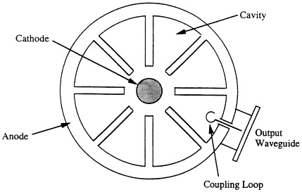
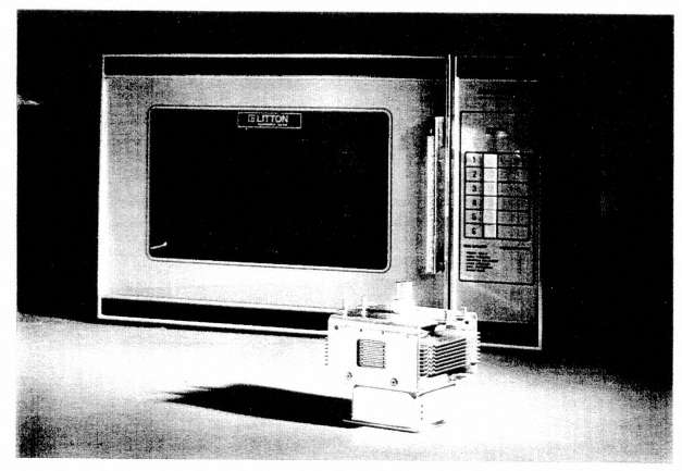
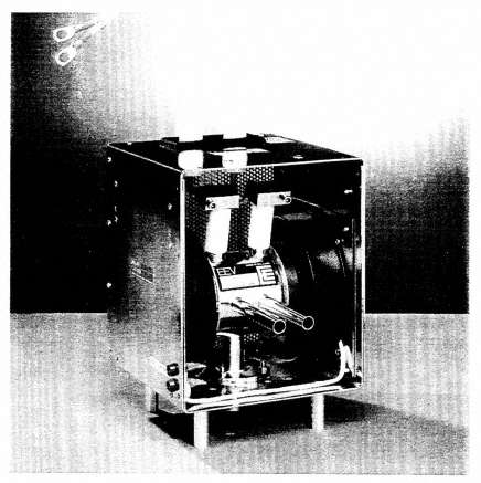
FIGURE 2-6 Industrial heating magnetron. (Photo courtesy of English Electric Valve Company, Limited).
(plasma heating) and capable of more than 2 MW of output in the 30 MHz range. Such tubes achieve their capability through application of pyrolytic graphite grid structures, an array of which is shown in Figure 2-7.
Specialty Tubes (Klystron, Gyrotron)
The other classes of microwave tubes will be selected for use only for those specialized requirements not fulfilled by the magnetron or power-grid tube, that is, when there is a need for very high continuous wave power (klystron) or very high continuous wave power at very high frequency (gyrotron).
Klystrons range in length from an inch or two to as long as 25 feet and operate at voltages from a few hundred to several hundred thousand volts. They power most modern radars (both civilian and military), special material processing equipment, and the linear accelerators used in science (e.g., at the Stanford Linear Accelerator Center) and medicine (e.g.,
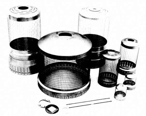
FIGURE 2-7 Pyrolytic graphite grid structures for power grid-tubes.
for radiation cancer therapy). Efficiencies as high as 80 percent have been achieved, although 50—60 percent is more common.
The gyrotron is large, heavy, and expensive and employs very high voltages and high magnetic fields generated by superconducting solenoids. However, the can do what no other robe has done——generate very high power levels at millimeter wavelengths. Much of the initial gyrotron development was sponsored by the Department of Energy to find a source for plasma hinting in fusion reactors (tokamak). Gyrotrons are driving such plasmas in Japan, Europe, and the former Soviet Union, and in the United States at Princeton University and General Atomics.
Material processing is able to benefit from this long and expensive development. Equipment operating at 28 GHz, 60-kW continuous wave power is available at Oak Ridge National Laboratory as well as Tokyo, Japan. Much higher power and frequency have been demonstrated and could be made available if the technical and economic studies warrant the investment. Currently, high-power tubes are operating at 60 GHz, 110 GHz, and 140 GHz. A large experimental gyrotron has achieved 500 kW at 110 GHz.
WAVE PROPAGATION
Microwave propagation in air or in materials depends on the dielectric and the magnetic properties of the medium. the electromagnetic properties of a medium are characterized by complex permittivity ![]() and complex permeability (μ), where:
and complex permeability (μ), where:
and
The real component of the complex permittivity, ![]() , is commonly referred to as the dielectric constant. since, as will become evident in this report,
, is commonly referred to as the dielectric constant. since, as will become evident in this report, ![]() is not constant but can vary significantly with frequency and temperature, it will be referred to simply as the permittivity (Risman, 1991). The imaginary component of complex permittivity,
is not constant but can vary significantly with frequency and temperature, it will be referred to simply as the permittivity (Risman, 1991). The imaginary component of complex permittivity, ![]() , is the dielectric loss factor. similarly, the real and imaginary components of the complex permeability, μ' and μ'', are the permeability and magnetic loss factor, respectively.
, is the dielectric loss factor. similarly, the real and imaginary components of the complex permeability, μ' and μ'', are the permeability and magnetic loss factor, respectively.
Wave Equations and Wave Solutions
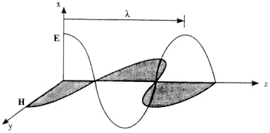
In wave propagation, if z is the direction of wave propagation and t is the time, the amplitude of the electric field and that of the magnetic field vary sinusoidally in both z and t. The number of complete cycles in a second is the frequency, f, and the distance that the wave travels in a complete cycle is the wavelength, λg. Hence, the frequency and the wavelength specify how a wave behaves in time and in distance.
It is instructive to illustrate the principles of wave phenomena by considering, in detail, a plane wave (Figure 2-8). A plane wave's wave-front is a plane normal to z with fields that are uniform in x and y. The wave has an electric field Ex in the x direction and a magnetic field, Hy in the y direction. For simplification, it is assumed that ![]() and μ = μ', since the real part of
and μ = μ', since the real part of ![]() or μ is much larger than the imaginary part. Once the wave properties are calculated by this approximation, the approximation can be improved by taking the imaginary components of
or μ is much larger than the imaginary part. Once the wave properties are calculated by this approximation, the approximation can be improved by taking the imaginary components of ![]() and μ as a perturbation.
and μ as a perturbation.
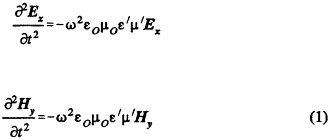
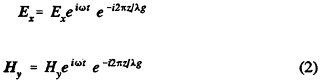
for a wave traveling forward in the + z direction and
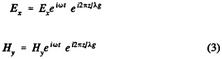
for a backward (-z) traveling wave. The wave has a time-dependence in ω, where ω is the angular frequency and is equal to 2πf, where f is the frequency in cycles/second or hertz. It has a z dependence in 2π/λg, which is called the wave constant.
If the dielectric medium is lossy, a complex ![]() must be used. Taking
must be used. Taking ![]() instead of
instead of ![]() in Equation 1, the wave solution for the forward wave is then:
in Equation 1, the wave solution for the forward wave is then:
where, the attenuation constant α is
Equation 5 indicates that the amplitude of the wave decreases exponentially as it propagates i.e., wave energy is dissipated during the propagation.
For the isotropic medium considered here, one remarkable property of the wave is that it carries an equal amount of energy in the electric and magnetic fields. For the plane wave, in any plane normal to z, the electric energy density is ![]() , and the magnetic energy density is
, and the magnetic energy density is ![]() . Since they are equal,
. Since they are equal,
Therefore,
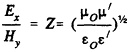
The ratio of Ex to Hy, or Z in Equation 6 is called the wave impedance . It characterizes the transverse electric-and magnetic-field profile of the wave and is thus also known as the
characteristic impedance, or the intrinsic impedance. In air or a vacuum, ![]() and Z is 377 ohms. Another remarkable property of microwaves is that at any plane normal to z, the electric and magnetic fields are in phase. The wave impedance is thus a real quantity and has the same value anywhere along the z axis.
and Z is 377 ohms. Another remarkable property of microwaves is that at any plane normal to z, the electric and magnetic fields are in phase. The wave impedance is thus a real quantity and has the same value anywhere along the z axis.
The power flow in the z direction is then,
The vector quantity, Pz z, is the Poynting vector, which is the power flow carded by the wave. The unit vector z indicates that the power flow points in the z direction.
In writing the dielectric constant ![]() as a complex quantity
as a complex quantity ![]() , the real component,
, the real component, ![]() , affects the wavelength in Equation 4 and the impedance in Equation 6, while the imaginary component,
, affects the wavelength in Equation 4 and the impedance in Equation 6, while the imaginary component, ![]() , represents the dielectric loss indicative of the microwave power absorbed by the medium and converted into heat.
, represents the dielectric loss indicative of the microwave power absorbed by the medium and converted into heat.
Standing Waves
The two remarkable properties of wave propagation stated earlier are that the wave carries an equal amount of the electric and magnetic energy and that the wave impedance stays constant in the propagation direction. These are intrinsic properties of transmission lines and are true as long as the forward and the backward traveling wave are separate. However, these conditions no longer hold when both the forward and backward traveling waves exist simultaneously. Consider the case that a conducting plane is placed at z=zL, causing reflection of a backward traveling wave. Adding Equation 2 and Equation 3 together and considering the fact that the electric field must be zero and the magnetic field is maximum at the conducting plane,
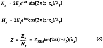
Both the electric and magnetic fields are in the form of a standing wave in the sense that all the energy carried by the wave forward is reflected back and that the wave is neither moving the energy forward nor backward. The wave impedance, Z, is no longer a constant and it varies as a tangent function in z.
Reflection and Transmission Coefficients
In the above case, a wave is reflected by placing a conducting plane at zL. A reflection also occurs when there is a discontinuity in the dielectric or magnetic property of the medium. In this case, however, only a portion of the wave is reflected. Consider the case in which a boundary separates two media with ![]() , μ1, and
, μ1, and ![]() , μ2 and wave impedances of Z1 and Z2, respectively.
, μ2 and wave impedances of Z1 and Z2, respectively.
Let an incident wave of an amplitude 1 volt/m travel forward in medium 1 normal to the boundary (Figure 2-9). Both Z1 and Z2 are real quantifies; the reflected wave in medium 1 has an amplitude (K-1)/(K+1) volt/m and the wave transmitted into the medium 2 has an amplitude 2K/(K+1) volt/meter, where K=Z1/Z2. The ratio (K-1)/(K+1) is called the reflection coefficient, and the ratio 2K/(K+ 1) is called the transmission coefficient . At the boundary, the sum of the tangential electric (magnetic) field of the incident wave and that of the reflected wave are equal to the tangential electric (magnetic) field of the transmitted wave.
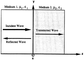
FIGURE 2-9
Schematic representation of reflection and transmission of a normal incidence electromagnetic wave.
WAVEGUIDE MODES
Microwaves can be divided into three types (Figure 2-10). For the transverse electromagnetic (TEM) wave, all fields are transverse. It is an approximation of the radiation wave in free space. It is also the wave that propagates between two parallel wires, two parallel

FIGURE 2-10 Waveguides - TEM, TE, and TM waves.
plates, or in a coaxial line. The parallel wires, or more precisely, twisted pairs, and the coaxial lines are used in the telephone industry. The transverse electric (TE or H) wave and the transverse magnetic (TM or E) wave are those in waveguides, which are typically hollow conducting pipes having either a rectangular or a circular cross section. In the TE wave, the z component of the electric field is missing, axed in the TM wave, the z component of the magnetic field is missing. Complicating the matter further, each TE. and TM wave in a waveguide can have different field configurations. Each field configuration is called a mode and is identified by the indexes m an n. In mathematics, those indexes are the eigenvalues of the wave solution.
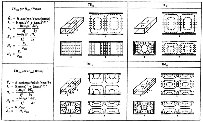
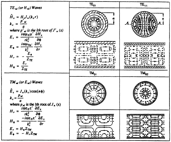
Field distributions for various modes of propagation in rectangular and cylindrical waveguides are available in standard text books (Ramo and Whinnery, 1944; Iskander, 1992). TEmn and TMmn modes are considered in rectangular waveguides and TEnl and TMnl modes are considered in cylindrical waveguides, where the indices m, n, and 1 are the order of the modes. Mathematically, they can be any integer, 0, 1, 2, etc. However, depending upon the size of the waveguide, physical reality allows only the lower values of m, n, and 1 and thus limits the
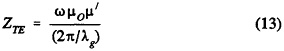
number of the modes that can exist in a waveguide. For the rectangular waveguides, the TM wave (or E wave) has the field components Ex, Ey, Ez, Hx, and Hy, and the TE wave (or H wave), the field components Ex, Ey, Hx, Hy, and Hz. For the cylindrical waveguides, the TM wave has the field components Er, EΦ Ez, Hr, and HΦ, and the TE wave, Er, EΦ, Hr, HΦ, and Hz. The rectangular waveguide has a height ''b'' in y and a width "a" in x, and the cylindrical waveguide has a radius, "a." Wave propagation is always in the z direction. Figures 2-11 and 2-12 show the field distributions of some lower-order waveguide modes. In the figures, electric fields are represented by solid lines and magnetic fields by dashed lines. Here again, the wave carries an equal amount of the energy in electric and magnetic fields. Since not all the fields are transverse, the energy carried by the z component of the field must be taken into the calculation. To calculate the energy, energy density is integrated over the cross-section of the waveguide. At any plane normal to z, the transverse electric field is always normal to, and in phase with, the transverse magnetic field. The wave impedance, which depends upon the transverse fields only, is again constant anywhere along the waveguide. The two transmission-line properties described earlier for the plane (TEM) wave, then, apply equally well to the TE and TM waves.
Wavelength and the Wave Impedance
The field distributions in Figures 2-11 and 2-12 are quite complex. In general, at a conducting surface, electric field lines are normal to the surface, and magnetic field lines are parallel to it. Away from the surface, all field lines follow continuity. Before carrying out calculations of the field distributions, the wavelength and the wave impedance of a waveguide mode will be considered. A rectangular waveguide will be used as an illustration.
For simplicity it is assumed that ![]() and μ = μ'. The solutions obtained in those conditions can be extended to the general case by the perturbation method when both
and μ = μ'. The solutions obtained in those conditions can be extended to the general case by the perturbation method when both ![]() and μ are complex. Both the wavelength and the wave impedance depend upon the dimensions "a" and "b" of the cross-section as well as
and μ are complex. Both the wavelength and the wave impedance depend upon the dimensions "a" and "b" of the cross-section as well as ![]() and μ' of the medium. Fortunately, the calculation can be simplified by defining a parameter k1, which depends upon only
and μ' of the medium. Fortunately, the calculation can be simplified by defining a parameter k1, which depends upon only ![]() and μ' of the medium, and another parameter Kc, which depends upon only the dimensions "a" and "b." Thus,
and μ' of the medium, and another parameter Kc, which depends upon only the dimensions "a" and "b." Thus,
and
The equations 9, 11, 12, and 13 above are true for all waveguides. Consider first the calculation of the wavelength in Equation 11. The wavelength must be real and positive by definition. That is true only when kc is smaller than k1. The waveguide mode indices, m and n, can be any integer including zero, but both cannot be zero. Since kc involves m and n, only a limited number of combinations of the values of m and n can keep kc smaller than k1. The number of the modes that can propagate in a waveguide is therefore limited. For small values of "a" and "b" such that the condition kc < k1 cannot be met, no waveguide mode can exist, and the waveguide is at cutoff frequency. For some moderate values of "a'' and "b," only one mode satisfies the condition kc < k1, and the waveguide is called a single-mode waveguide. For very large values of ''a" and "b," thousands of the modes satisfy the condition, and the waveguide is a multimode waveguide.
Field Distributions
The expressions listed in the left columns of figures 2-11 and 2-12 are used to calculate field distributions. Also plotted in those figures are the field distributions of some lower-order modes in rectangular and cylindrical waveguides. Consider specifically a TM wave in a rectangular waveguide (Figure 2-11). The first expression in the "TM wave" column of Figure 2-11 is a functional form for the z component of the field, Ez. The second expression is the calculation of kc discussed earlier in Equation 10. Knowing kc, the next two expressions in the column calculate Hx and Hy. The wavelength is calculated from Equation 11, and finally, Ex and Ey are calculated from the wave impedance, ZTM, given in Equation 12. The field distribution in the waveguide is thus completely determined.
INTERACTIONS BETWEEN MICROWAVES AND MATERIALS
When an electric field interacts with a material, various responses may take place. This section discusses the interactions of a variety of materials with microwave fields. Coupling mechanisms, critical electrical properties (and their variability with temperature and frequency), and the resulting conversion of incident electromagnetic energy into process heat are discussed in some detail. Also, heat transfer and related problems of uneven heating and thermal runaway are covered.
In conductors, electrons move freely in the material in response to the electric field and an electric current results. Unless it is a superconductor, the flow of electrons will heat the material through resistive heating. However, microwaves will be largely reflected from metallic conductors and therefore they are not effectively heated by microwaves.
In insulators, electrons do not flow freely, but electronic reorientation or distortions of induced or permanent dipoles can give rise to heating. The complex permittivity is a measure of the ability of a dielectric to absorb and to store electrical potential energy, with the real permittivity, ![]() , characterizing the penetration of microwaves into the material, and the loss factor,
, characterizing the penetration of microwaves into the material, and the loss factor, ![]() , indicating the material's ability to store the energy. The loss tangent, tanδ, is indicative of the ability of the material to convert absorbed energy into heat. For optimum
, indicating the material's ability to store the energy. The loss tangent, tanδ, is indicative of the ability of the material to convert absorbed energy into heat. For optimum
coupling, a balanced combination of moderate ![]() to permit adequate penetration and high loss (maximum
to permit adequate penetration and high loss (maximum ![]() and tanδ) are required.
and tanδ) are required.
Materials that are amenable to microwave heating are polarizable and have dipoles that reorient rapidly in response to changing electric field strength. However, if these materials possess low thermal conductivity and dielectric loss that increases dramatically as the temperature increases "hot spots" and thermal runaway may be experienced.
Materials considered in this report are diverse, including metal-like materials, ceramics, polymers, glass, rubber, and chemicals. The principal effect of microwave interaction is the heating of materials. The committee thus considers the conversion of microwave energy into heat, a process that involves interaction between microwave fields and the conductivity or dielectric properties of the material. Interactions between microwaves and materials can be represented by three processes: space charges due to electronic conduction, ionic polarization associated with far-infrared vibrations, and rotation of electric dipoles (Newnham et al., 1991).
The processes described above may be illustrated in combination by considering a material that has an electronic conduction σe, an ionic conduction σi, and a complex permittivity, ![]() . In the presence of an electric field, E, in the material, a current must flow.
. In the presence of an electric field, E, in the material, a current must flow.
According to the Maxwell equations, the current density j is
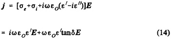
where,
The phase angle, δ, relates to the time lag involved in polarizing the material. The quantity tanδ is the loss tangent, the most important parameter in microwave processing. Returning to Equation 14, the first term at the fight of the equation is the component of the current 90 degrees out of phase with the electric field. It is the displacement current that stores electric energy in the material. The average electric energy stored per unit volume is
The second term at the right side of Equation 14 is the component of the current that is in phase with the electric field. Through this term, the microwave energy is converted into heat energy for material processing. The average power per unit volume converted into heat is,
Hence, the loss tangent characterizes the ability of the material to convert absorbed microwave power into heat with absorption depending on electric field intensity, frequency, loss factor, and permittivity. A "lossy" material (high tanδ and ![]() ) heats more effectively than a low-loss (low tanδ and
) heats more effectively than a low-loss (low tanδ and ![]() ) material.
) material.
Conductive Losses
Electronic conduction can play a key role in the microwave heating of metal-like materials or semiconductors. As shown in Table 2-2, materials with moderate conductivity heat more effectively-than either insulating or highly conductive materials. Low-loss insulators are difficult to heat from room temperature, even though microwave penetration is significant. However, many oxide ceramics have resistivities that decrease rapidly with increasing temperature affording more efficient coupling (Newnham et al., 1991). As discussed later in this chapter and in Chapter 5, the rapid change in loss can lead to uneven heating and thermal runaway. Electronic conductivity does not vary significantly with the frequency in the microwave frequency range. The temperature dependence of the conductivity varies widely with the material depending on the dominant transport mechanism.
When the conductivity of the material is very large, the fields attenuate rapidly toward the interior of the sample due to skin effect. The skin effect involves the magnetic properties of the material. When a large current flows inside the sample due to a high conductivity, a combination of the magnetic field with the current produces a force that pushes conducting electrons outward into a narrow area adjacent to the boundary. The extent of this skin-arm flow is called the skin depth, ds. Skin depth is defined as the distance into the sample at which the electric field strength is reduced to 1/e (Risman, 1991). The derivation is available in standard text books (Ramo and Whinnery, 1944; Iskander, 1992).
Skin depth ranges from several microns to a few meters. For example, at 2.45 GHz, brass and graphite have skin depths of 2.6 and 38 μm respectively and cured epoxy and alumina have skin depths of 0.73 and 187 m, respectively. When the skin depth is larger than the dimension of the sample, the effect may be neglected. In the opposite case, penetration of microwave energy will be limited, making uniform heating impossible.
Even though ions are thousands of times heavier than electrons and are chemically bonded into the network, ionic conduction losses are important in materials such as silicate
Table 2-2 Heating characteristics of a range of compounds (Newnham et al., 1991; Walkiewicz et al., 1988)
|
Material |
Resistivity (Ω;-m) |
Heating Characteristic (ºC/min-temperature reached in specified time at 1 kW and 2.45 GHz) |
|
Metal Powders |
10-8 -10-6 |
Moderately Heated |
|
Al |
|
577ºC/6 min |
|
Co |
|
697/3 |
|
Cu |
|
228/7 |
|
Fe |
|
768/7 |
|
Mg |
|
120/7 |
|
Mo |
|
660/4 |
|
Sulfide Semiconductors |
10-5 -10-3 |
Easily Heated |
|
FeS2 |
|
1019/6.75 |
|
PbS |
|
956/7 |
|
CuFeS2 |
|
920/1 |
|
Mixed Valent Oxides |
10-4 -10-2 |
Easily Heated |
|
Fe304 |
|
1258/2.75 |
|
CuO |
|
1012/6.25 |
|
C0203 |
|
1290/3 |
|
Ni0 |
|
1305/6.25 |
|
Carbon and Graphite |
~10 |
Easily Heated |
|
Alkali Halides |
104 10-5 |
Very Little Heating |
|
KCl |
|
31/1 |
|
KBr |
|
46/.25 |
|
NaCl |
|
83/7 |
|
NaBr |
|
40/4 |
|
LiCl |
|
35/0.5 |
|
Oxides |
104 -1014 |
Very Little Heating |
|
SiO2 |
|
79/7 |
|
Al2O3 |
|
78/4.5 |
|
KAlSi3O8 |
|
67/7 |
|
CaCO3 |
|
74/4.25 |
glasses (Newnham et al., 1991). At low frequencies, ions move by jumping between vacant sites or interstitial positions in the network, giving rise to space charge effects. At higher frequencies, vibration losses, such as those from vibration of alkali ions in a silicate lattice, become important. Ionic conductivity does not vary much with the microwave frequency. Because ionic mobility is an activated process, the conductivity increases rapidly with temperature.
Atomic and Ionic Polarizations
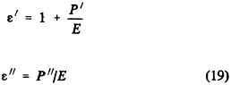
Under an electric field, E, the electron cloud in an atom may be displaced relative to the nucleus, leaving an uncompensated charge-q at one side of the atom and +q at the other side. The uncompensated charges produce an electric dipole moment and the sum of those dipoles over a unit volume is the polarization, P. Similarly, deformation of a charged ion relative to other ions produces dipole moments in the molecule. Those are the atomic and ionic polarizations induced by the electric field. Although atomic and ionic polarizations occur at microwave frequencies, they do not contribute to microwave heating.
In terms of the polarization, ![]() may be written as:
may be written as:
Hence,
Therefore, in principle, the polarization contributes to both ![]() and
and ![]() . However, as shown schematically in Figure 2-13, atomic and ionic polarization mechanisms are active to optical and infrared frequencies, respectively. They act so fast that the net polarization observed under an electric field at microwave frequencies is in phase with the field. As a result, both P'' and
. However, as shown schematically in Figure 2-13, atomic and ionic polarization mechanisms are active to optical and infrared frequencies, respectively. They act so fast that the net polarization observed under an electric field at microwave frequencies is in phase with the field. As a result, both P'' and ![]() are zero, and thus, atomic and ionic polarizations do not generally contribute to microwave absorption.
are zero, and thus, atomic and ionic polarizations do not generally contribute to microwave absorption.
Losses associated with lattice or molecular vibrations in the infrared region due to the interaction of microwaves with dipoles are observed in alkali halides and in some polymer and composite systems (Newnham et al., 1991). These frequency shifts, or lower-frequency tails, are due to weaker bonding and heavier masses of heavy ions in the alkali halides, and to long-chain vibrations and weak interchain bonding forces in polymers.
FIGURE 2-13 Frequency dependence of the several contributions to the polarizability schematic (Kittel, 1959).
Dielectric Materials and Electric Polarizability
In electronic conduction, either free motion of the electrons or collective diffusion of the ions is assumed. As the charge particles move, a current is induced. The situation is quite different in dielectric materials. Instead of the motion of the electrons or ions, electric dipoles play a dominant role in the properties of the material.
The mechanism of polarizability that causes the microwave absorption involves rotation and orientation of the dipoles (Kittel, 1959; Debye, 1929). There are three ways this can happen in a solid:
-
The single atom can have the shape of the "electron cloud" surrounding the nucleus distorted by the electric field. In general, atoms with many electrons (high atomic number) are more easily distorted and are considered more "polarizable."
-
Molecules with a permanent electrical dipole will have the dipole aligned in response to the electric field.
-
Molecules, with or without a permanent dipole, can have bonds distorted (direction and length) in response to an electric field.
Without an electric field, the dipoles are randomly oriented and the net polarization is zero. In a static field, the dipoles align with the field and the polarization is maximized. These dipoles can rotate, but they rotate against a friction force. As the frequency of the electric field increases, the rotation of the dipoles cannot follow, and the net polarization in the material is no longer in phase with the electric field. In that case, it follows from Equation 15 that the polarization contributes both ![]() and
and ![]() . In terms of Debye's dielectric relaxation theory (Debye, 1929):
. In terms of Debye's dielectric relaxation theory (Debye, 1929):
Substituting Equation 20 into Equation 19:
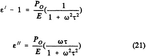
The quantifies ![]() and
and ![]() are represented in Figure 2-14. The relaxation time, τ, is the time interval characterizing the restoration of a disturbed system to its equilibrium configuration after a microwave field has been applied. The behavior of τ determines the frequency and temperature dependences of
are represented in Figure 2-14. The relaxation time, τ, is the time interval characterizing the restoration of a disturbed system to its equilibrium configuration after a microwave field has been applied. The behavior of τ determines the frequency and temperature dependences of ![]() and
and ![]() and varies widely in liquids and in solids. In water at room temperature, τ is about 5×10-11 s. The peak of the absorption, that is, the peak of
and varies widely in liquids and in solids. In water at room temperature, τ is about 5×10-11 s. The peak of the absorption, that is, the peak of ![]() , is thus at the microwave wavelength of 1 cm. The absorption band is very broad. An interesting feature of this model is that the absorption disappears both at very low and very high frequencies, which explains very well the properties of water (Kittel, 1959). For polymers, τ is on the order of 10-7 seconds (Hawley, 1992). The unique feature of this model is that the effect of the polarization in both
, is thus at the microwave wavelength of 1 cm. The absorption band is very broad. An interesting feature of this model is that the absorption disappears both at very low and very high frequencies, which explains very well the properties of water (Kittel, 1959). For polymers, τ is on the order of 10-7 seconds (Hawley, 1992). The unique feature of this model is that the effect of the polarization in both ![]() and
and ![]() diminishes altogether above the microwave frequency.
diminishes altogether above the microwave frequency.
The broad range of possible material properties that can be effectively processed using microwaves is illustrated by Table 2-3, showing representative dielectric properties of a sampling of important materials. Data needed for microwave process control or numerical simulations would require much more extensive information about the effect of temperature, frequency, and physical characteristics on the properties, as well as knowledge about heat-transfer responses. Although some excellent reviews exist for some materials (Bur, 1985; Westphal and Iglesias, 1971; Westphal and Sils, 1972; Westphal, 1975; 1977; 1980), there is a paucity of available data for both processors and heating-system designers.
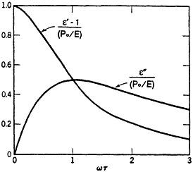
FIGURE 2-14 Frequency dependence of real and imaginary parts of the dielectric constant in the Polarization-Orientational Model (Kittel, 1959).
TABLE 2-3 Representative Dielectric Properties of Selected Materials.
|
Material |
Frequency (GHz) |
|
tan δ |
Temp. (C) |
Reference |
|
Raw Beef |
3.0 |
48.3 |
0.28 |
20 |
(Thuery, 1992) |
|
Frozen Beef |
2.45 |
4.4 |
0.12 |
-20 |
|
|
Potato (78% water) |
3.0 |
8.1 |
0.38 |
25 |
|
|
Al2O3 |
3.6-3.8 |
9.02 |
0.00076 |
25 |
(Westphal and Iglesiad, 1971) |
|
|
|
9.69 |
0.00128 |
500 |
|
|
|
|
10.00 |
0.00930 |
700 |
|
|
BN |
8.52 |
4.37 |
0.00300 |
25 |
|
|
Si3N4 |
8.52 |
5.54 |
0.00360 |
25 |
|
|
Polyester |
8.5 |
3.12 |
0.0028 |
25 |
(Westphal and Iglesias, 1971) |
|
PTFE (Teflon) |
2.43 |
2.02 |
0.00042 |
25 |
(Andrade et al., 1992) |
|
PEI (Ultem) |
1.0 |
3.05 |
0.003 |
25 |
(Bur, 1985) |
|
Epoxy |
1.0 |
3 |
0.015 |
25 |
(Bur, 1985) |
|
Concrete (dry) Concrete (wet) |
1.0 1.0 |
6.57 13.2 |
0.530 0.485 |
25 25 |
(Westphal and Iglesias, 1971) |
Depolarization Factors
In a dielectric material, as the sample is polarized under an applied electric field, surface charges appear at the sample boundary (Figure 2-15). The surface charges produce a depolarization field opposing the applied field. The net field inside the sample is thus reduced, while the field outside the sample remains the same. The computation in this case involves a depolarization factor, N, listed in Table 2-4, which is simple only if the sample has an ellipsoidal shape and has its major axis placed either parallel or normal to the electric field. Fortunately, a cylinder may be considered an elongated ellipsoid and a disc, a fiat ellipsoid. Taking the depolarization factor, N, into account, the relation between the field inside the sample, E in, and that outside, Eext, is (Kittel, 1959; Becker, 1964):
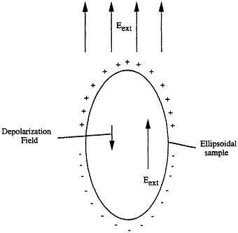
FIGURE 2-15 The field outside the sample Eext and that inside is the sum of Eext and a depolarization field (adapted from Kittel, 1959).
When ![]() is large, the electric field inside the sample could be reduced to zero. The sample is then completely shielded from effects of the microwaves. To avoid this, surface charges must be reduced. This could be accomplished by using a slender cylinder or a thin disc placed parallel to the electric field (N=0). Due to either skin effect or depolarizing fields, microwave heating of bulk materials that have very large conductivity or permittivity is very difficult.
is large, the electric field inside the sample could be reduced to zero. The sample is then completely shielded from effects of the microwaves. To avoid this, surface charges must be reduced. This could be accomplished by using a slender cylinder or a thin disc placed parallel to the electric field (N=0). Due to either skin effect or depolarizing fields, microwave heating of bulk materials that have very large conductivity or permittivity is very difficult.
TABLE 2-4 Depolarization Factors, N
|
Shape of the sample |
Depolarization Factor, N |
|
Sphere |
1/3 |
|
Thin slab normal to the field |
1 |
|
Thin slab parallel to the field |
0 |
|
Long cylinder parallel to the field |
0 |
|
Long cylinder normal to the field |
1 |
Thermal Runaway
The discussion of microwave fundamentals has focused on the generation and propagation of microwaves and their interaction with materials. However, the thermophysical behavior of the sample must also be understood. Stable microwave heating depends on the rate of microwave power absorption and on the ability of the sample to dissipate the resulting heat, that is, if the temperature dependence of the power absorption is less than the temperature dependence of the heat dissipation at the surface of the specimen (plus insulation system), stable heating should be observed. The rapid rise in dielectric loss factor with temperature is the major issue in thermal runaway and temperature nonuniformity. Therefore, although microwave heating frequently is touted as providing more uniform heating, nonuniform heating is a reality in many materials, often at nominal heating rates.
Some attempts have been made to quantify the conditions under which thermal runaway occurs and how it can be controlled. Roussy et al. (1985; 1987) predicted that heating rubber specimens above a certain power level was unstable, and that temperature increased uncontrollably, while below that power level the temperature came to a steady state. The regime in which stable heating occurred was mapped in terms of the heat loss and acceleration of power absorption with temperature rise. Stable heating was possible with rapid heat removal (i.e., no insulation) or small temperature dependence of the dielectric loss factor. Tian et al. (1992) used computer simulation of two-dimensional temperature distributions in microwave-heated alumina ceramics to predict that up to certain power levels, stable heating in both uninsulated and insulated specimens would occur. As expected, the critical power levels were greater in uninsulated specimens. The use of insulation significantly accelerated both the heating rate and the risk of thermal runaway.
Kriegsmann (1992) modeled heating of uninsulated ceramic slabs and cylinders. Taking account of the effect of material properties on the microwave field within the materials, but ignoring temperature gradients, it was determined that, over a certain incident power range, the
part temperature is a multivalued function of incident power resulting in an S-shaped power-temperature response curve (Figure 2-16). Below the critical power level, the sample will heat in a stable manner to a steady-state value on the lower branch of the response curve. If the power is increased to exceed the upper critical power, the temperature will jump to the upper branch of the temperature—power curve. These observations have been supported by modeling work performed to simulate microwave heating of alumina (Barmatz and Jackson, 1992; Johnson et al., 1993). These studies emphasize the importance of sample size, geometry, relative density, and composition.
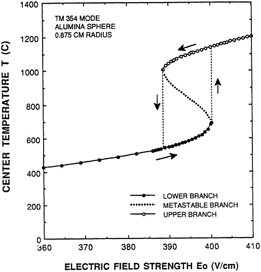
FIGURE 2-16 Predicted power——temperature response curve for an alumina sphere (courtesy of M. Barmatz, Jet Propulsion Laboratory).
Due to rapidly increasing dielectric loss factor, the area of the sample that first exceeds the critical temperature will continue to heat rapidly at the exclusion of the rest of the sample. Thus, process control schemes to control thermal runaway depend upon knowing the temperature at the interior of the specimen. While it may be that precision is more important than accuracy for this control, many of the problems of temperature measurement discussed in Chapter 3 will influence the processor's ability to control the process. Moreover, in industrial practice, it is not usually possible to insert a thermocouple or optical probe into the specimen.


