
3
Scientific Rationale for Watershed Research
WATERSHEDS AS ENVIRONMENTAL LABORATORIES
The goal of hydrologic science is to understand and predict the fluxes and storages of water over a range of space and time scales. Such understanding also is necessary to comprehend and predict fluxes and storages of sediments and solutes and to evaluate the suitability of the aquatic environment for living organisms. Experimentation is an essential part of science; in order to understand a phenomenon, it must be measured. Although many individual components of the hydrologic cycle (e.g., free-surface flow, porous media flow, evaporation, chemical transport) can be studied in the laboratory under carefully controlled conditions, the partitioning of rainfall into interception, infiltration, direct surface runoff, evaporation, and ground water recharge, taking into account the natural temporal and spatial variability of rainfall and soil and vegetative characteristics, can be observed in a meaningful way only at the watershed scale.
Scientists and laypersons alike are usually quite comfortable with the notion of laboratory research, but watershed research often has been viewed as collecting data for data's sake, with little scientific content. The major difference between watershed research and typical laboratory research involves the factors of complexity and control. A research or experimental watershed can be viewed as a special type of iconic "material model," just as a soil column in an indoor laboratory is a material model. To be sure, a watershed is much more complicated than a laboratory column, but it has many of the attributes required of material models. In general, a material model should be similar to but simpler than the prototype system and should provide the scientist with better control of the system and allow accurate measurements of inputs and outputs.
Carefully chosen research watersheds certainly can be simpler than
some generic watersheds. For example, watersheds can be chosen such that there is little or no surface runoff or little or no subsurface runoff. In addition, the instrumentation provided in the research watershed provides the scientist with data that would be impossible to obtain without it. Just as the laboratory scientist is not interested in the data from a soil column per se, but is interested in how these data can be used to provide insight into the physical, chemical, or biological processes involved in a general system, the watershed scientist is not specifically interested in data from the watershed as would be the case for a monitoring activity. Both are interested in using the data obtained to improve intellectual or mathematical models and to estimate or provide techniques for field estimation of model parameters for a general system. The most significant deficiency of a watershed as a laboratory is that it is impossible to design, control, and replicate inputs. Nevertheless, information gained from work on research watersheds is one of the keys to developing a comprehensive predictive watershed science that can be applied to solve water resource problems. The "iconic" experimental watershed models are necessary to develop, test, and refine the mathematical models that are required to generalize results from site-specific studies and ultimately to allow the U.S. Geological Survey (USGS) to provide the tools for solving important problems on watersheds outside a research watershed network and on watersheds influenced by human activity.
HYDROLOGIC MODELS
Rosenblueth and Wiener (1945) defined two classes of models: (1) formal or intellectual and (2) material. The formal models generally consist of mathematical descriptions of real-world phenomena, whereas material models, including iconic or "look-alike" and analog models, are real systems that either closely resemble the prototype or have the same mathematical representations. In contemporary hydrology the most commonly utilized models belong to the class of formal or intellectual models. Models are an essential part of scientific inquiry and engineering practice. They can serve as a platform and repository for integrating new scientific knowledge and process understanding as it is developed. They help to identify and guide data needs for problem evaluation. A coordinated program of model development, laboratory work, and field data collection can accomplish far more than any of these activities alone. Models, properly verified and confirmed with field data, can provide an effective basis for evaluation of alternative management strategies and decision support.
Most hydrologic models consist of sets of linked ordinary or partial
differential equations expressing various conservation laws along with appropriate initial and boundary conditions that must be consistent with the mathematical equations and system geometry. In most cases it is impossible to obtain analytical solutions to the sets of equations, so they are numerically solved on digital computers. To obtain numerical solutions, the continuous solution domain of the problem (which may include up to three space dimensions and time) is replaced by a grid function, and the solution to finite difference equations or finite element approximations is sought at this finite number of points. Several assumptions and approximations are required to formulate digital hydrologic models. First, a decision must be made regarding the scope (space and time) of the model and the variables to be considered. Second, decisions must be made regarding the physical principles or laws to be included. For example, most models include the principle of conservation of mass, some include conservation of momentum, and some include conservation of energy. Then equations are derived that reflect these principles and that also include certain empirical relationships such as Darcy's Law or Manning's equation. At this stage, many assumptions typically are introduced. For examples, rainfall rate is assumed to be a continuous input variable in space and time rather than consisting of discrete drops, watershed surfaces are assumed to be homogeneous, and the soil is assumed to be a homogeneous porous medium. Initial and boundary conditions consistent with the scope of the problem and with meeting the mathematical requirements of the sets of equations must then be specified. Finally, the grid or mesh structure must be specified and the appropriate equations solved.
Hydrologic models often are classified as lumped or distributed. In a lumped model the spatial independent variables are eliminated by assuming spatial or volumetric averages of dependent variables and parameters. Thus, lumped models consist of sets of ordinary differential equations. Distributed models, on the other hand, retain spatial variables, so they consist of linked partial differential equations. In most cases the distributed models are simplified by eliminating one or two spatial dimensions, which may introduce serious distortions.
A significant problem associated with hydrologic modeling is that of spatial variability of inputs, parameters, and variables at length scales smaller than the computational length scale. The seriousness of this problem is dependent on the scale of the system being modeled and the scale of variability relative to the computational scale. A valid research question that can only be answered with a combination of experimental watershed data and mathematical models is: "Can procedures developed to scale up from a watershed of 0.1 square kilometers to one of 10 square kilometers give
insight into techniques required to scale up from 10 square kilometers to 100 square kilometers or greater?" A second problem that is particularly important in modeling the transport and fate of chemical constituents is that of specifying the initial conditions. For example, a model for nitrate transport through an agricultural watershed quickly "forgets" the initial conditions with respect to water stored in the soil, but the quantity, position, and chemical form (e.g., organic or inorganic) of nitrogen may be extremely important in attempting to evaluate the effect of changed agricultural practices on nitrate concentration and fluxes in the saturated zone.
For effective use in policy analysis, strategy selection, or engineering design, hydrologic models must be firmly founded on a strong base of observational data. Such data are essential to ensure that the model theory and structure are consistent with real-world behavior as well as conditions at the specific site where the model is applied. Observational data also are essential to test and confirm the predictive capability of the model for its intended application.
A BRIEF HISTORY OF WATERSHED RESEARCH
The importance and necessity of watershed-scale research have been recognized since early in the century. Research watersheds were established by the U.S. Forest Service near Wagon Wheel Gap, Colorado, in 1910 (Bates and Henry, 1928) and by the Soil Conservation Service in agricultural areas in 1935. The objectives of the early watershed studies were to determine the effects of various forest and agricultural management practices on water yields, flood peaks, and erosion losses. The "paired watershed" concept was often used to evaluate the effects. This technique required measurements of streamflow at two similar (and preferably adjacent) watersheds over a calibration period until a reliable statistical relationship between the streamflow characteristics of the two watersheds could be established. Then treatments were imposed on one of the watersheds and any changes in the statistical relationship were evaluated over the treatment period. Scientific reasoning then attempted to ascribe the mechanism(s) responsible for the changed relationship. Subwatersheds and small plots within these watersheds often were instrumented in an attempt to understand the pathways and dynamics of water flow.
Problems of scale and spatial variability of precipitation, soil, and vegetation became apparent very early and led to the establishment of much larger experimental watersheds by the Agricultural Research Service (ARS) of the U.S. Department of Agriculture during the period 1955–1965. These
watersheds and associated Watershed Research Centers were established in major physiographic and climatological regions of the United States and were intended both as representative watersheds and as field laboratories.
USGS watershed studies have a relatively short history in comparison to the agency's basic hydrologic data collection activities. Its first effort at systematic watershed research began in 1958 with the initiation of the Hydrologic Benchmark Network (HBN) (Cobb and Biesecker, 1971). The HBN came about at a time when the scientific community was concerned about the lack of a robust information base, or benchmark, for differentiating natural hydrologic and geochemical variations and changes from those due to human activities. Such a benchmark was considered vital to the development of effective environmental regulations, especially in those days prior to the enactment of the National Environmental Policy Act.
The HBN provided a nationwide network of small headwater basins that were unaffected by human activities and that were expected to remain so for many decades, thereby providing nearly pristine conditions for the study of natural hydrologic processes and trends (Cobb and Biesecker, 1971). From the beginning, however, the HBN suffered from insufficient funding. As a result, it has never been able to support a focused program of long-term, process-oriented watershed research. Indeed, it has not even been able to sustain a data collection effort sufficient to answer many hydrologic process-and trend-related questions. Currently, USGS is considering a redesign of the HBN—one that is capable of providing a more limited but more useful base of information related to benchmark hydrologic conditions.
A second USGS program of watershed investigations began in the early 1980s in conjunction with the National Acid Precipitation Assessment Program. A limited number of USGS Atmospheric Deposition and Analysis (ADA) sites were established, which, like HBN, tended to be in small headwater basins. The aim was to evaluate hydrologic and geochemical processes in basins where the only human effects or inputs to the basin would be those transported into the basin through the atmosphere. In particular, the ADA watersheds were oriented toward understanding the transport, fate, and long-term patterns of the two primary atmospheric deposition chemical species, sulfur and nitrogen.
The ADA watersheds have been successful intensive process research sites in terms of both scientific productivity and longevity. Most are still operating, although most have expanded their scientific focus beyond the atmospheric deposition issue. Importantly, these watersheds, with their emphasis on the intensive monitoring and analysis of water and geochemical cycling, follow the pattern established by the Forest Service at such sites as Hubbard Brook, New Hampshire and Coweeta, North Carolina, and the
Agricultural Research Service at the Little Washita, Oklahoma.
More recently, as part of the U.S. Global Change Research Program, USGS established a network of five Water, Energy, and Biogeochemical Budget (WEBB) research watersheds at Loch Vale, Colorado; Luquillo Experimental Forest, Puerto Rico; North Temperate Lakes, Wisconsin; Panola Mt., Georgia; and Sleepers River, Vermont. These sites were designed to improve (1) understanding of the processes controlling terrestrial water, energy, and biogeochemical fluxes, process interactions, and process relations to climatic variables and (2) the capability to predict terrestrial water, energy, and biogeochemical budgets over a range of spatial and temporal scales (Lins, 1994). The five watersheds represent diverse geographical and environmental settings and include sites that had a preexisting base of multidisciplinary research activities. For example, two WEBB watersheds are associated with National Science Foundation Long-Term Ecological Research sites—one is in a Forest Service Experimental Forest, and one is in a national park. Strong collaborative research relationships with scientists in other federal agencies as well as the academic community are a noteworthy characteristic of WEBB research activities.
The types of research being conducted at the WEBB watersheds include hillslope hydrology and geochemistry, water quality genesis, flow path delineation, physical and chemical weathering processes, hydrologic processes at different scales, and effects of seasonal freezing and snowpack on soil trace-gas fluxes, among others. Clearly, these activities have importance for issues other than global change, particularly water quality. The WEBB sites in the future will have to address a more diverse scientific agenda if they are to remain responsive to agency needs. Research watersheds are becoming too expensive for any one program or issue to sustain for more than a decade. Accordingly, for the WEBB, ADA, or HBN watersheds to remain valuable enough to warrant continuation, the USGS must begin utilizing such sites as generic research resources and abandon their use as single-issue field sites.
As new water-related problems emerged, they were either addressed at existing experimental watersheds or new watersheds were established to obtain the required data. For example, during the 1960s, several urban watersheds were instrumented (e.g., Putnam, 1972) and several studies were begun to evaluate the effects of drastic disturbance, such as surface mining on water yields, erosion, and water quality (e.g., Musser, 1970). As the potential for environmental damage by pesticides became apparent, existing watersheds, such as those operated by the ARS in Coshocton, Ohio, were utilized to make some of the first measurements of the quantities of pesticides reaching streams. Much of this early work has been summarized by Stewart,
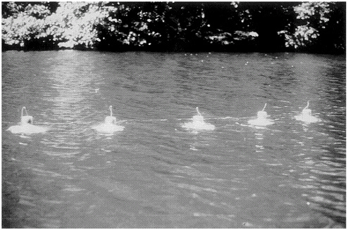
Gas sampling array for monitoring methane flux from lake and reservoir sediments through the water and into the atmosphere. There is growing evidence that lake and reservoir sediments are a major carbon sink worldwide. Source: U.S. Geological Survey.
et al. (1976).
During the 1960s, significant advances were made in the speed and storage capacity of computers, and the trend in hydrologic research shifted from experimental watersheds to development of sophisticated mathematical models of watershed behavior. Ideally, the model developments should have stimulated new and better field measurements and this was true to some extent. However, when budgets leveled off or declined in the 1970s, many experimental watersheds were closed, and in some quarters it was thought that activities at experimental watersheds were primarily oriented to data collection and that enough watershed data had been obtained. As models were critically tested using data from experimental watersheds, the scientific community has again recognized the importance of watershed research. The National Research Council's Committee on Opportunities in the Hydrologic
Sciences concluded that ''hydrologic science is currently data-limited'' and that "Interest in ever-increasing scale has outrun the financial support for observation, and the balance of hydrologic science is now seriously skewed toward modeling. It is important that observation and analysis proceed hand in hand" (NRC, 1991). This fact had been recognized a decade earlier by the renowned USGS hydrologist Walter Langbein. The "ability to solve complex mathematical systems has now outpaced understanding of the physical, chemical and biological processes, or even the appropriate data". (Langbein, 1981, emphasis added).
Throughout the late 1980s and into the 1990s, federal agencies have been experimenting with new prototypes of watershed management processes. These processes integrate traditional water resource management objectives, such as flood damage reduction, water supply, and navigation with environmental objectives such as water quality, soil erosion reduction, ground water recharge, and biodiversity conservation. Multiple-objective processes require a much more complex analysis of watershed hydrology than the engineering designs of the past, which assumed essentially static quantities of water moving through the system (water quality was generally not addressed), simple storage reservoirs, and trapezoidal channels. The new approaches, in contrast, must account for the natural landscape heterogeneity that supports ecological communities; the chemical transformations that affect water quality; and the complex interactions between water molecules, soil, and air that facilitate ground water recharge and control soil erosion rates if they are to support environmental objectives effectively.
DIRECTIONS FOR USGS ACTIVITY IN WATERSHED SCIENCE
The work of the USGS is both regional and national in scope; consequently, the agency requires efforts that are distributed across the entire country, through a range of climatic and physiographic regions. As will be discussed further in Chapter 4, the committee believes that the USGS should use information from research watersheds and data from assessment programs to build effective modeling and data synthesis efforts to move toward an integrated set of activities to address problems of importance to the nation. Just one aspect of such an integrated program—operating research watersheds—represents a potentially massive investment. The USGS cannot single handedly create and run research watersheds across the country. Fortunately, many agencies and organizations (including the USGS) currently operate research watersheds (Table 3.1), so the USGS can draw on a wealth of data and experience from an array of investigations. Further, the USGS should
develop and encourage collaborative efforts with the universities Water Resources Institutes, and the 40 cooperative units of the Biological Resources Division. Involvement of students would contribute to both the USGS project and the training of water resources professionals for the future.
Despite a fairly widespread geographic distribution of research watersheds, it does not follow that all information adequate for addressing the most critical water resource and water-related environmental problems is being provided. The USGS should assess its programs and direct future efforts to help fill gaps in the knowledge base in watershed science to ensure that policy decisions can be informed by solid scientific results. In Chapter 4 the committee presents its views of gaps in the scientific knowledge base that might be targets in strategic planning for future work by the USGS.
TABLE 3.1 Summary of Active Experimental Watersheds in the United States
NOTE: Most research watersheds supported through the U.S. Forest Service (FS), U.S. Department of Agriculture (USDA), and the National Science Foundation's Long-Term Ecological Research (NSF-LTER) sites are included here. Other active research watersheds operated, for example, by university researchers are not included. All cooperators may not be listed for some watersheds.
|
Research Site and Agencies Involved |
No. of Watersheds |
Watershed size Range (ha) |
Data Collection History (yr) |
|
|
ALASKA |
||||
|
Arctic Tundra NSF |
2 |
Up to 14,300 |
Up to 12 |
1, 2, 4, 6, 7, 9, 10 |
|
Bonanza Creek NSF |
1 |
7,500 |
3 |
4,9 |
|
ARIZONA |
||||
|
Beaver Creek USDA-FS |
1 |
111,300 |
Up to |
|
|
Santa Rita USDA-ARS, Univ. of Ariz. |
8 |
1.05–4.0 |
Up to 21 |
1, 2, 7, 9, 10 |
|
Walnut Gulch |
25 |
0.34–14,937 |
Up to 42 |
1, 2, 6, 7, 9 |
|
CALIFORNIA |
||||
|
Caspar Creek Calif. Depts. of Fish and Game and Forestry, USDA-FS, |
1 |
907 |
|
|
|
Univ. of Calif. |
||||
|
Chamise Creek NBS, NPS |
1 |
4.3 |
Up to 15 |
1, 2, 4, 5, 6, 8, 9 |
|
East Fork of the Kaweah |
||||
|
River NBS, NPS, USGS |
3 |
16,000 |
1 |
1, 2, 4, 8, 9, 10 |
|
Emerald Lake NPS, NOS, NASA, USGS |
1 |
133 |
Up to 15 |
1–9 |
|
Log and Tharp's watersheds NPS, NBS, USGS, FS |
2 |
13.1–48.9 |
Up to 15 |
1, 2, 4, 5, 6, 8, 9 |
|
San Joaquin Experimental |
||||
|
Range Calif. State Univ., Fresno, USDA-FS |
1 |
138 |
Up to 60 |
|
|
COLORADO |
||||
|
Loch Vale NPS, USGS |
1 |
660 |
Up to 15 |
1–10 |
|
Niwot Ridge NSF |
1 |
546 |
8 |
1, 2, 4, 6, 9, 10 |
|
Research Site and Agencies Involved |
No. of Watersheds |
Watershed size Range (ha) |
Data Collection History (yr) |
|
|
GEORGIA |
||||
|
Little River, Ga. USDA-ARS |
6 |
1,594–33,460 |
Up to 28 |
1, 2, 4, 6, 7 |
|
Panola Mountain USGS |
1 |
41 |
12 |
1–9 |
|
Watkinsville USDA-ARS |
5 |
1.26–7.8 |
Up to 56 |
1, 2, 3, 6, 7, 8, 9 |
|
IDAHO |
||||
|
Reynolds Creek USDA-ARS |
9 |
0.9–23,379 |
Up to 33 |
1, 2, 3, 6, 7, 8, 9 |
|
IOWA |
||||
|
Treynor USDA-ARS, Iowa State Univ. |
5 |
6.0–60.7 |
Up to 32 |
1–9 |
|
KANSAS |
||||
|
Konza Prairie NSF |
5 |
85–10,600 |
Up to 12 |
1–9 |
|
MISSOURI |
||||
|
Centralia USDA-ARS, Univ. of Mo. |
3 |
1,230–7,238 |
Up to 27 |
1–6 |
|
MISSISSIPPI |
||||
|
Goodwin Creek USDA-ARS, Univ. of Miss. |
14 |
6.1–2.141 |
Up to 14 |
1–9 |
|
Nelson Farm USDA-ARS, Univ. of Miss. |
3 |
1.6–2.0 |
Up to 7 |
1, 2, 3, 6, 7, 8 |
|
Holly Springs SUDA-ARS, Univ. of Miss. |
2 |
1.3–1.8 |
3 |
1, 2, 4, 5, 6, 7, 8, 9 |
|
NEW HAMPSHIRE |
||||
|
Hubbard Brook USDA-FS, NSF |
1 |
13.2 |
Up to 38 |
1–9 |
|
NEW MEXICO |
||||
|
Sevilleta NSF |
2 |
250–350,000 |
Up to 36 |
1, 2, 4, 6, 7, 9 |
|
NORTH CAROLINA |
||||
|
Coweeta USDA-FS, NSF |
15 |
<10–760 |
Up to 60 |
1–10 |
|
Research Site and Agencies Involved |
No. of Watersheds |
Watershed size Range (ha) |
Data Collection History (yr) |
|
|
OHIO |
||||
|
Coshocton USDA-ARS, Ohio State Univ. |
24 |
0.26–122.6 |
Up to 59 |
1–9 |
|
OKLAHOMA |
||||
|
Little Washita USDA-ARS, Okla. State Univ. |
5 |
0.47–52,834 |
Up to 33 |
1, 2, 4, 5, 6, 7, 8 |
|
El Reno USDA-ARS |
8 |
1.62 |
20 |
1, 2, 4, 5, 6, 7, 8, 9 |
|
Ft. Cobb USDA-ARS |
2 |
2.1–2.55 |
14 |
1, 2, 4, 5, 6, 7, 8, 9 |
|
Woodward USDA-ARS |
4 |
2.7–5.56 |
19 |
1, 2, 4, 5, 6, 7, 8, 9, 10 |
|
OREGON |
||||
|
H.J. Andrews USDA-FS, NSF |
9 |
Up to 6,400 |
Up to 11 |
1, 2, 4, 6, 7, 8, 9, 10 |
|
PENNSYLVANIA |
||||
|
Mahantango Creek USDA-ARS, Penn. State Univ. |
3 |
718–41,970 |
Up to 67 |
1, 2, 3, 6 |
|
SOUTH CAROLINA |
||||
|
North Inlet NSF |
1 |
53 |
Up to 11 |
1, 2, 4, 6, 9 |
|
TEXAS |
||||
|
Riesel USDA-ARS |
18 |
0.10–125 |
Up to 59 |
1, 2, 4, 5, 6, 7, 8, 9 |
|
VERMONT |
||||
|
Sleepers River USACE, USGS |
4 |
47–11,160 |
Up to 35 |
1–8 |
|
WASHINGTON |
||||
|
West Twin Creek NPS, NBS, FS, Univ. of Wash. |
1 |
58 |
Up to 11 |
1, 2, 4, 5, 6, 8, 9 |
|
WISCONSIN |
||||
|
North Temperate Lakes NSF, USGS |
1 |
12,000 |
Up to 75 |
1–10 |


