
8
The Dynamic Atmosphere: Unraveling the Contributions of the Earth's Subsystems
The mass of the atmosphere is only about 10-6 that of the Earth, so the atmosphere's contributions to the Earth's static gravity field, although observable, are much smaller than those from the solid Earth. The atmosphere, though, is highly mobile. Cyclones and atmospheric tides cause the mass of the atmospheric column to vary by 1 to 10%. Consequently, gravity measurements at an accuracy 10-8 or better will contain an atmospheric signal. Indeed, the atmosphere contributes a significant fraction of the Earth's total time-dependent gravity field and is one of the largest sources of time-dependent signal at periods of about 1 year and less.
The importance of the atmospheric signal at a period of one year can be seen from the degree amplitude results shown in Figure 8.1. These have been estimated from ECMWF analyses and are shown superimposed on the satellite errors for a 5-year solution. The atmospheric signal is one of the larger annually-varying signals we have considered (cf. Figure 4.5)—it rises above the SST and SSI errors up to degrees of 28 and >40, respectively. In fact, the annually-varying atmospheric gravity signal has already been identified in the lowest-degree zonal gravity coefficients using satellite laser ranging to LAGEOS (Figure 8.2) (e.g., Yoder et al., 1983; Chao and Au, 1991; Nerem et al., 1993a, b; Gegout and Cazenave, 1993; Chao and Eanes, 1995; Dong et al., 1996).
Because the atmospheric signal is so large, it is a potential source of error when using satellite gravity to learn about other processes. This has been discussed in general in Chapter 1 and has been further addressed for each relevant geophysical application in later chapters. In summary, uncertainties in atmospheric pressure data used to remove the atmospheric signal from the gravity estimates are large enough that they could sometimes be the dominant error source for hydrological or glaciological estimates. They are usually not apt, however, to limit seriously the scientific value of those estimates.
Because the uncorrected atmospheric effects are a large time-dependent signal in the gravity data, it is of interest to understand the origin of the atmospheric signal in its own right. Accordingly, in the remainder of the chapter we describe the general characteristics of the atmospheric pressure field.
The global mean surface pressure is close to 984.5 mbar (Trenberth and Guillemot, 1994) and has an annual cycle of about 0.45 mbar (Trenberth 1981; Van den Dool et al., 1995), with a maximum in July that is caused by variable atmospheric water loading (Chen et al., 1996). By differencing the July and January climatologies, one can derive the peak-to-peak magnitude of the annual cycle (Figure 8.3). At least three redistributions of atmospheric mass can be identified: (1) between land and ocean, (2) between the
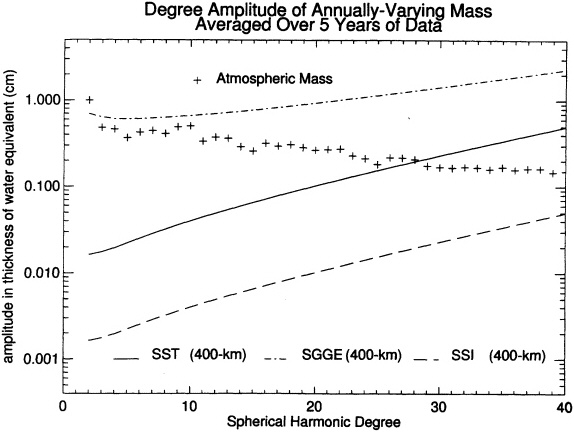
FIGURE 8.1 The degree amplitudes in mass, expressed as the thickness of a water layer, for the annually-varying terms in the atmosphere. The atmospheric results are inferred from ECMWF pressure data from 1992-1993. The results for the satellite errors assume a 5-year satellite mission. The units on the y-axis are approximately equivalent to mbar of pressure.
Southern and Northern Hemispheres, and (3) between high elevations, such as the Tibetan Plateau, and lower elevations. These mass variations are caused by differential heating of the Northern and Southern Hemispheres and the land and the ocean (Van den Dool and Saha, 1993; Saha et al., 1994) and, as such, they are the mass counterparts of the monsoons. The mass redistributions are sufficiently large, both in terms of the pressure difference (20 mbar = ~200 mm of water) and the spatial scale, and they move sufficiently slowly to be detectable from space.
Other prominent regular features in the atmosphere are the diurnal and semi-diurnal solar tides. The departure of the surface pressure from the daily mean at a specific universal time is an expression of propagating tides (Figure 8.4). The tides are up to 2.5 mbar but exhibit both regular changes (April and October appear to have the strongest tides) and irregular changes. Although the tides move too quickly to be observed directly by gravity measurements, they are an important source of noise and, through their near-resonances with some orbits, can produce long-period (observable) perturbations to orbital elements. In Sun-synchronous measurement systems like the proposed gravity missions, it is important to know how the tides alias into lower frequencies.
Figures 8.3 and 8.4 display "climatology" or normal variations. Departures from normal variations can be large (up to about 50 mbar) and can occur over a wide spectrum of temporal and spatial scales, particularly at high and mid-latitudes (Figure 8.5). These anomalies drift around, decay, develop, and merge, usually with a slight net eastward phase speed at mid-latitudes, and a net westward phase speed at low lati-
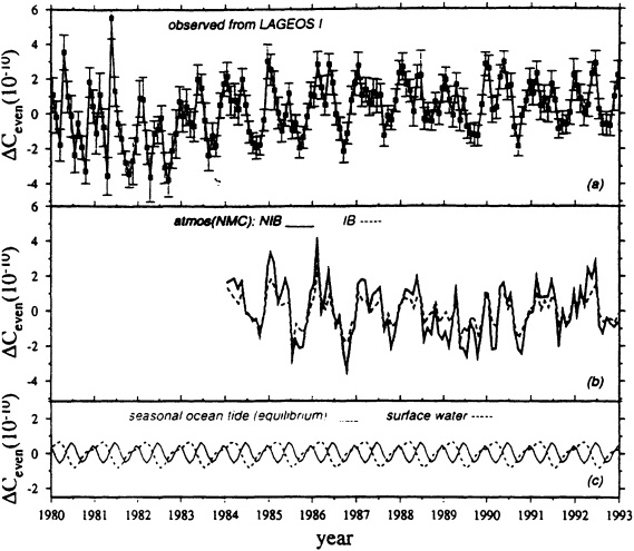
FIGURE 8.2 (a) Monthly Ceven (even zonal harmonics of the Earth's gravity field) series spanning 1980-1992 recovered from LAGEOS I satellite laser ranging data (the mean value has been removed). The error bars represent a I sigma uncertainty.
(b) Monthly Ceven calculated from NMC (1984-1992) atmospheric surface pressure data using the same linear combination of the spherical harmonic coefficients to which the observations are sensitive. Solid line: NIB model; dashed line: IB model.
(c) Monthly Ceven calculated from an equilibrium seasonal ocean tide model (solid line) and the surface water (dashed line) results of Chao and O'Connor (1988). Figure from Dong et al. (1996).
tudes. This is a reflection of the chaotic nature of weather. Some anomalies are quasi-persistent, existing for weeks or months. Surface pressure anomalies in the tropics are small (a few mbar)—exceptions include hurricanes, which cause pressure anomalies of up to 100 mbar for a short time.
There are many atmospheric phenomena that cause variations in pressure—Table 8.1 lists those that will likely be sensed by a gravity satellite. The list is not exhaustive and does not include phenomena that are unlikely to significantly influence gravity. For purposes of modeling, each phenomenon is presented in terms of a spatially-isolated mass anomaly, with its characteristic diameter on the Earth's surface, magnitude (in mbars of surface pressure), and typical lifetime and speed. These specifications were used to generate the atmospheric curves in Figure 1.2.
The geographic structure of, and dynamical mechanisms responsible for much of the atmospheric contribution to time-dependent gravitational anomalies have not yet been fully explored. A possible source for these effects on seasonal time scales, for example, might be the Indian monsoon system, which involves large mass transfers between the Asian continent and
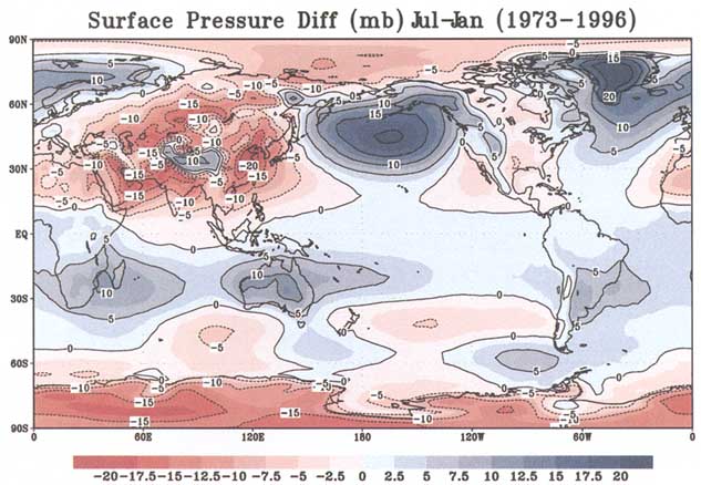
FIGURE 8.3 The difference between the surface pressure climatologies for July and January, showing the peak-to-peak variation due to the atmospheric annual cycle in mass. Contour interval is 5 mbar. Blue values are positive, red values are negative. The climatology is a multi-year average for the month in question, based on recent reanalysis at NCEP (Kalnay et al., 1996).
surrounding ocean areas, capable of inducing significant local gravity anomalies. While concomitant atmospheric pressure perturbations over the oceans would be redistributed more or less uniformly by the inverted barometer effect (see Chapter 4), the large land-ocean mass flux involved in this and other seasonal phenomena may be capable of inducing an average pressure change over the surface of the world oceans that could have a significant impact on the global gravitational field.
On short time scales, intraseasonal variability includes the important effects of cold (blocking) outbreaks over mid-latitude continents (cf. Figure 1.2), and the effects of the eastward-propagating surface pressure waves associated with the tropical Madden-Julian Oscillation. At interannual time scales the El Niño-Southern Oscillation (ENSO) phenomenon dominates global-scale atmospheric variability, with concomitant meridional redistribution of atmospheric wind and mass fields (e.g., Dickey et al., 1992; Mo et al., 1997).
The detection of atmospheric gravitational effects is not likely to be an important goal of time-dependent gravity studies because of the continued generation of high-quality pressure fields by meteorological forecast centers. Although it is possible that satellite gravity constraints on atmospheric pressure over data sparse regions (e.g., parts of the Southern Hemisphere such as Antarctica) could provide results that are more accurate than those available from meteorological analyses and that such results could be used as a proxy data type in reanalysis efforts (e.g., Kalnay et al., 1996), extending barometric networks on the surface would most likely provide the best return on available resources (see Chapter 7).
The better recovery of certain non-atmospheric signals could also greatly enhance atmospheric modeling capabilities. Particularly promising are the hydro-
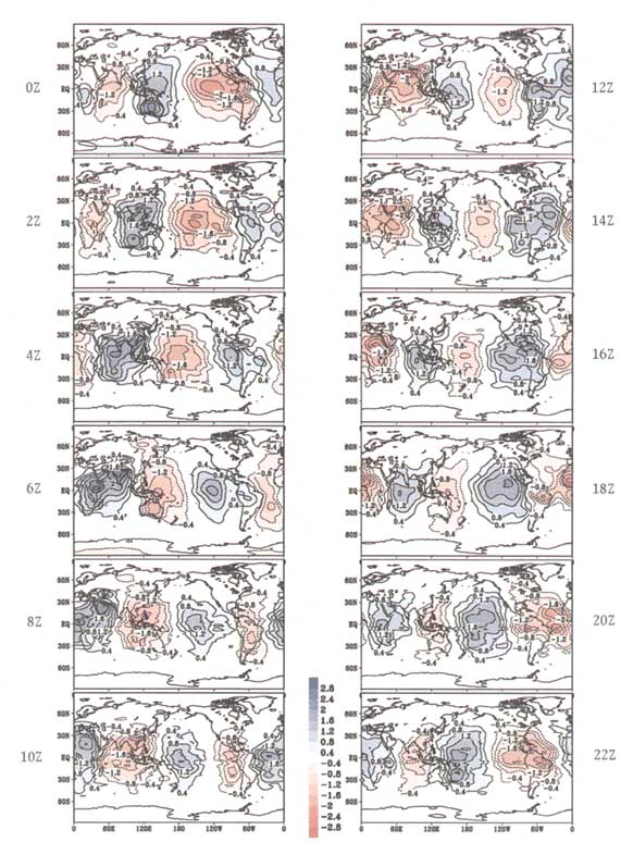
FIGURE 8.4 The climatological daily cycle in surface pressure for the month of January, showing the westward motion of atmospheric tides. Contour interval is 0.4 mbar (no zero line). Red is negative and blue is positive. Each panel shows the surface pressure at a given time of day minus the daily mean. Based on recent reanalysis at NCEP (Kalnay et al., 1996). The reanalysis output at 0, 6, 12 and 18Z has been interpolated as in Van den Dool et al. (1996).
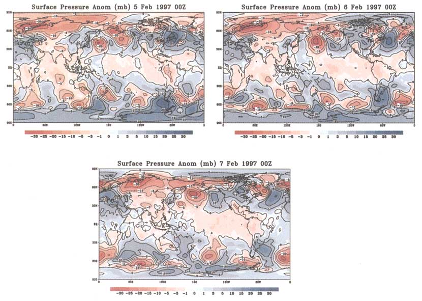
FIGURE 8.5 The surface pressure minus the February climatology on three successive days (OZ only) in February 1997, showing the irregular weather con atmospheric mass variations. Figure calculated according to real-time NCEP analyses. Contour interval is 5 mbar. Red is negative and blue is positive.
TABLE 8.1 Weather and Climate Phenomena, Expressed as Anomaly Mass Discs, that Likely have a Bearing on Temporal Gravity Variations.
|
Feature |
Diameter (km) |
Magnitude |
Time scale |
Motion |
|
Mid-latitude cyclone |
500-2,000 |
10-50 mbar |
=10 days |
=20 m/s irregular |
|
Mid-latitude anticyclone |
1,000-3,000 |
10-40 mbar |
=15 days |
=10 m/s |
|
Atmospheric blocks |
2,000-3,000 |
20-30 mbar |
10-50 days |
little at high mid-latitude, often a cutoff low on equatorward side |
|
30-60 waves or Madden-Julian tropical oscillation |
5,000-10,000 |
<10 mbar |
|
5-10 m/s |
|
Precipitation events1 |
100-500 |
0.1-10 cm per event |
hours if runoff, weeks if slow evaporation, melting |
after deposition: virtually no motion |
|
Atmospheric tides |
10,000 |
=2 mbar |
daily, regular |
one revolution around the Earth in a day |
|
Annual cycle 1 (air shuttle between land and sea, monsoon) |
10,000 |
10 mbar |
365 days |
none, standing-type oscillation |
|
Annual cycle 2 (air shuttle from Northern to Southern Hemisphere) |
40,000 |
2 mbar |
365 days |
none, standing oscillation |
|
Annual cycle 3 (air shuttle from high to low terrain and back a half year later) |
3,500 |
few to 10 mbar |
365 days |
none |
|
Southern Oscillation |
5,000-10,000 |
a few mbar |
months to years |
none, seesaw of mass between tropical Indian Ocean and Pacific |
|
North Atlantic Oscillation |
3,000-8,000 |
=10 mbar |
days to years |
none, seesaw of mass between Iceland low and Azores high. |
|
Pacific North American pattern |
3,000-6,000 |
=10 mbar |
days to months (weaker power out to years) |
none2 |
|
1 The accumulated effect of several events may have larger diameters (approximately 1/4 of United States) and longer time scales (months). 2 Chain of mass anomaly centers over the Pacific and North America; adjacent centers are opposite in sign. |
||||
logical applications described in Chapter 6. Reliable, extended-range forecasting and simulation is possible only through interactive coupling to water conditions in soils and the ocean. To the extent that a gravity mission improves models for the hydrosphere, therefore, meteorology will benefit in turn.
CONCLUSIONS
-
Knowledge of atmospheric variations is vital to unraveling the effects of the other subsystems (such as the hydrological cycle) involved in gravity variations. With increasing accuracy in gravity measurement, precise knowledge of the uncertainty in atmospheric surface pressure at seasonal, annual, and secular time scales becomes increasingly important
-
Reliable, extended-range forecasting, which would require interactive coupling between the atmosphere and the water in soils and the ocean, would benefit from the hydrological constraints discussed in Chapter 6.
-
Satellite gravity measurements with high temporal and spatial resolution may improve the atmospheric databases and models both as a proxy data type and for verification in areas where atmospheric measurements are lacking and water levels are constant It would be more effective, however, to have a global network of barometers, sufficient to remove the atmospheric signals from the gravity data.


