
2
Climate Models, Observations, and Computer Architectures
2.1 MODEL CONSTRUCTION
The internal cycling of the different elements in the Earth system and their interaction and feedback with the other elements ultimately creates climate. Creating models that characterize climate requires information about the various subcycles in order to characterize the interactions and feedbacks ( Box 2-1) and the resulting amplification or dampening influences on the climate. Individual boxes and arrows ( Figure 2-1 ) are useful for demonstrating how the integration of the individual elements of the environmental system ultimately produces a model for climate.
In general, each component of the climate system (atmosphere, ocean, land, ice) is modeled separately. Oceanographers build models inputting such information about the oceans as bottom and coastal topography, total amount of water and total salt content. In response to time-dependent inputs of freshwater (as rainfall and river runoff), momentum fluxes, and heat fluxes at the surface the models calculate the distribution of salinity, temperature, momentum (currents), density, and sea ice in the oceans over time.
Similarly, atmospheric scientists build models of the atmosphere incorporating surface geography and orography and the amount and distribution of gases in air (N2, O2, CO2, H2O and the more minor gases). In response to the input of radiation from the sun, to boundary conditions of specified time-dependent sea-surface-temperature (SST) and land surface
|
Box 2-1 Feedbacks in Climate Models type, and to the distribution of industrial and other anthropogenic aerosols and gases, the atmospheric models calculate: Feedbacks in the climate system occur when the output from one component is input into a second component, which then generates an output altering the first component. For example, increasing ambient air temperatures cause higher sea-surface temperatures, which result in decreased CO2 dissolution into the oceans, leading to higher atmospheric CO2 concentrations, which increases ambient air temperature. Climate models are constantly adjusted to account for the multiple non-linear feedbacks, which are common in nature. |
-
the time-dependent distribution of temperature and pressure,
-
momentum (winds),
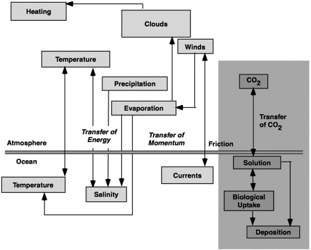
FIGURE 2-1 A representation of the major coupling mechanisms between the atmosphere and ocean subsystems. The processes in the shaded area are being developed offline. (Figure adapted from McGuffie and Henderson-Sellers, 1997. “A Climate Modelling Primer.” Figure 1-3 John Wiley and Sons, New York.)
-
precipitation,
-
cloudiness,
-
humidity,
-
radiation within the atmosphere and at the lower boundary,
-
the total infrared radiation escaping to space.
Land specialists build models containing factors influencing the distribution and runoff of water on the surface, soil moisture, the growth of vegetation (which in part determines land albedo, the amount of evapotranspiration, and the uptake of carbon dioxide) and include the geography and topography of the land surface. In response to time-dependent inputs of radiation, water, gases, and winds from the atmosphere, the models calculate the time-dependent temperature, vegetation type, soil moisture, snow cover, and runoff. Modeled biogeochemical cycles describe the exchange of carbon, constituents of nitrogen and sulfur between the biosphere, ocean, and atmosphere.
These different component models are incorporated into the climate models, which use the interaction and feedbacks among the different cycles to describe the temporal state of the climate. For example, fluxes of water and momentum delivered from the atmosphere to the ocean in part determine the sea-surface temperature, which in turn influences the atmospheric temperature. The coupling of these components forms a global climate model.
One of the goals in climate modeling is to calculate the properties and evolution of the climate system in response to forcings, which represent the external changes in the components of the system, affecting climate. Changes in solar output, the effective changes in solar radiation reaching Earth caused by alterations in the orbital parameters of Earth, and change in volcanic emissions of aerosols are clearly forcings external to the climate system. External forcings include those that are specified even when they are internal to the climate system. Thus, specified changes in the chemical composition of the atmosphere leading to alterations to the incoming or outgoing radiation are forcings within the climate system, but because they are specified rather than calculated, they are treated as external forcings. Forcings have both a natural and anthropogenic component ( Box 2-2).
2.2 OBSERVATIONS AND CLIMATE MODELS
Most of the information about the climate system derives from observations taken for purposes other than climate. For example, operational measurements of atmospheric temperature and humidity are routinely taken by a variety of means for the purpose of weather forecasting. Because the period of interest is very short (up to about 10 days), constant
|
Box 2-2 Humans and Climate Forcings Over the past 30 years, there has been increasing interest related to the role of humans in climate. Humans produce large amounts of gases and aerosols such as CO2, soot carbon, and SO42− aerosols that are capable of altering the radiation budget both directly and indirectly. Additionally, land-use practices alter the distribution of vegetation on continents thereby changing the albedo, or reflectivity, of the land surface. The impact of human activities on climate is strongly debated in both the scientific and political communities. One of the goals of climate modeling is to quantify the role of humans in forcing climate change. |
changes in the models and observing systems are made to improve the forecasts, but any change introduced into the system will cause a discontinuity that can be confused with a climate change. Also, cost saving measures for weather observations can put long time series, of major value for climate, in jeopardy. It was a conclusion of NRC (1999b) that our current ability to adequately document climate change was compromised by an observing system unsuitable to the task.
The basic properties required of a climate monitoring system as enumerated in NRC (1999b) were:
-
Changes to an observing network should be assessed in terms of the effects on climatic time series.
-
Any replacement instruments should be overlapped with the old ones for an appropriate period of time.
-
Metadata which documents the instruments and procedures should be kept and archived along with the data.
-
Data quality and homogeneity should be assessed as part of routine operating procedures.
-
The data should be used in environmental assessments of various types so that it will be constantly examined.
-
Historically important time series within the observing system should be maintained and protected.
-
Data poor or otherwise unknown or sensitive regions should receive special priority.
-
The entire system should be designed with climate and weather requirements in mind.
-
Commitment to old systems and a transition plan from research to operations needs to be a part of the system.
-
Every effort should be made to facilitate access and use of the data by national and international users.
A climate observing system is inadequate when it either fails to measure climatically important quantities or when the measured quantities do not satisfy the 10 properties above. By this standard there is not an adequate climate observing system. The existing weather observing system does not satisfy the 10 principles. Some important climatic quantities, such as subsurface ocean temperature and salinity, land soil moisture, and the concentrations of specific atmospheric species such as the hydroxyl radical, are either measured inadequately or are not measured at all.
An effective integrated system for producing and delivering climate information has as one of its major elements the climate observing system. To the extent our vision of coupled climate observations, high-end modeling, and research is the proper one, and to the extent that the relationships between the elements are as important as the elements themselves, one cannot solve the high-end modeling problem without solving the sustained climate observations problem. Because observations cost an order of magnitude more and the infrastructure to maintain sustained observations is again an order of magnitude more than any likely modeling infrastructure, the problem of producing and delivering climate information is, to first order, one of creating and maintaining a climate observing system.
Improving Climate Models with Observations
Climate models are built using our best scientific knowledge of the processes that operate in the atmosphere, ocean, land, and cryospheric systems, which in turn are based on our observations of these systems. Climate models and their gradual improvement therefore arise from the totality of the research enterprise, which can be diagrammed as shown in Figure 2-2. The climate system is observed, and on the basis of these observations, physical processes (e.g., the radiative and other thermal processes that determine the temperature) and the large-scale structure of the component systems are understood. Models of the component systems are constructed and compared to observations. When disagreements between models and observations are noted, model processes are improved, perhaps by performing field studies devoted to a single process (e.g., clouds) or perhaps to acquire a detailed set of observations of a set of interacting processes by which to improve the details of component models. The state and accuracy of climate models depends on the state of all the elements of Figure 2-2. It is in this sense that climate models contain our accumulated wisdom about the underlying scientific processes and can be no better than our observations of the system and our understanding of the processes that interact to form the climate.
Weather forecasting provides an example of a process for improving climate modeling based on the interactions of the elements in Figure 2-2.

FIGURE 2-2 Modeling paradigm.
Sustained global observations of the atmosphere have been taken for the last 50 years in support of weather forecasting. These observations are assimilated into a global atmospheric model, and an analysis of the current state of the atmosphere is performed in order to initialize a weather forecast. The skill of the forecast is primarily determined by the accuracy of this initial analysis, which in turn depends on the coverage of the observations, the quality of the observations, the accuracy of the models, and the accuracy of the data assimilation scheme.
The sequence of twice (or four times) daily analyses is normally what researchers consider “data,” but it is as close to an optimal blend of observations and model output as current science allows. Thus, weather prediction is the arena in which observations used to define climate are taken and archived, ultimately forming the basis for our knowledge of the climate of the interior of the atmosphere. Hollingsworth et al. (1999) have articulated the advantage of linking observations with forecasting; “The forecast centre's ability to compare every single instantaneous observational measurement with a forecast of that measurement is a powerful scientific resource.” This resource can be employed to improve the parameterization of processes in models, and to gauge the adequacy of the observing system ultimately improving the forecast models, and the skill of weather forecasts. A similar method to improve the parameterizations of processes consists of confronting models with data taken from field programs designed to illuminate physical processes not adequately resolved by routine weather observations. Combinations of the two methods can be used.
2.3 PURPOSES OF CLIMATE MODELING
Climate models are employed for a number of different purposes. Climate models as close to comprehensive as possible can be used to simulate the climate system. The model can be run for a long time and its annual cycle and variability about that annual cycle assessed. Once the model has proven itself in this simulation mode, simulations can be performed on the climate model, which clearly could not be performed on the climate. For example, the climate model can be used to simulate the response of the climate model to external changes, such as to the solar constant or to volcanic eruptions. The most common type of assessment is to increase the concentrations of carbon dioxide in a model according to the measured increase over the last 45 years and inferred increases before that. The response of the climate system to these changes, with or without external changes, can then be compared to the observed changes in order to infer the causes of whatever climate change has occurred. The climate model can then be run into the future to either examine the response to projected increases in the concentrations of radiatively active constituents or, in the case of comprehensive climate models, to examine the response to projected emissions of radiatively active constituents.
Coupled climate models can be used to probe for predictability on short time scales (months to years) when some data exists. Ideally, a coupled assimilation is performed using past data to achieve an initial analysis of the state of the coupled atmosphere-ocean-land system, and the system is allowed to run freely to give a (retrospective) prediction of the state of the climate. Because the data exists for the prediction period, these hindcasts can be used to determine what the skill of prediction would have been over a long series of forecasts if they had taken place prospectively instead of retrospectively. Once skill in hindcast mode is demonstrated, coupled climate models can be used to predict the climate a season to a year in advance.
Coupled climate models can be used to probe for predictability in the climate system on longer time scales when no observational data exists. A long simulation can be run and the model output treated as if it were true observational data. The method described above can then be used on the simulated model output, perhaps sampled at points for which observations could exist, and simulated predictions could be made. Comparing the predicted state of the climate to the simulated “true” future state (again perhaps sampled at the points of a presumed observational system) could give a rough guide to the existence of predictability.
A similar method could be used to guide the design of proposed observing systems. The state of the model climate is completely known in both space and time. The ability of various proposed observing systems to accurately describe the model climate could be tested by sampling the
model system at the proposed observation points with errors characteristic of actual observing systems.
Because the details of the climate are affected by weather noise that needs to be averaged out in climate assessments, climate ensembles must often be run. Ensembles usually include 10–30 members (see discussion in Section 5.1).
An important recent use for models is to downscale information from the resolution at which the climate is simulated by global models, to a much smaller region at much higher resolution in order to capture the local characteristics of the specific region. Output from the global climate model is used as lateral boundary conditions for much higher resolution regional atmospheric models that then capture the local peculiarities of terrain and orography and, ideally, return details on local weather and weather changes under different climatic regimes. Questions have arisen as to the consistency of this method because it does not allow the back reaction from the small to the large-scale.
2.4 COMPUTER ARCHITECTURES IN SUPPORT OF CLIMATE MODELING
Climate and weather modeling require enormous computing capacity and capability. Over the next few years the two supercomputer architectures that will provide this computing power are vector parallel processor machines (currently manufactured primarily in Japan) and microprocessor-based massively parallel computers (currently manufactured primarily in the United States) ( Box 2-4).
In a few years, high-end computer systems expected to be available internationally can be divided roughly into the following categories:
-
Clusters of nodes, each node having multiple shared-memory processors (SMP) running some variant of the Unix operating system. These server systems are composed of commodity processor and memory chips on nodes interconnected by custom-designed networks.
-
Loosely integrated clusters of PCs running the Linux operating system. “Linux clusters” are based on commodity PCs using standard PC processor and memory chips and interconnection networks built of commodity parts. These build-your-own systems are considerably cheaper per peak gigaflop than those in category 1, but they tend to be software poor and often suffer from reliability problems.
-
Computers based on an innovative and promising new architecture are being produced in limited quantities by TERA, a small U.S. company. The TERA computer uses specially designed processors that use dataflow concepts to support fine-grain parallelism; each processor supports up to 128 threads of execution to hide the latency of outstanding
|
Box 2-3 A quick tour of the computer terminology used in this report The heart of any computer is its processing element (PE; also known as ‘processor' or ‘central processing unit'). The PE can have multiple pipelines, each of which can evaluate floating-point operations in a sequence of stages, one stage per clock cycle. Each PE may have its own memory unit that only it can address directly, as in a normal personal computer (PC), or it may share access to a memory unit with several other PEs (see node). The PE may read from and write to memory directly, as in traditional vector processors like the Cray C90 and NEC SX-4, but this requires very high memory bandwidth. Cache-based microprocessors use memory chips that are very slow compared to those used in vector machines. To compensate, microprocessor-based computers place one or more levels of cache between the processor and memory units. Cache is a special memory unit that provides very fast access to and from the PE. If the datum needed by the PE resides in the highest-level (L1) cache, it can be retrieved from cache to the PE in only a small number of clock cycles. If not, a “cache miss” occurs and the request must then go to the next level (L2, etc.) of cache. If the datum is not in any level of cache, the request goes to the memory unit on the node. Each successive level of cache is progressively larger but takes longer for the requested datum to reach the PE. A node is a collection of two or more processors grouped together so that they share access to a common memory unit. This set of PEs is said to have uniform memory access to the entire unit of shared memory. A node has a single-system image because only a single copy of the operating system needs to be stored in memory to be shared by all the PEs. A collection of nodes connected by a network is said to have distributed shared memory if the computer's architecture supports direct reading or writing by a PE of data stored in memory units on the other nodes. Such a computer also has a single-system image. If inter-node communication can only take place via messages that must be handled by the PEs, then the computer simply has distributed memory. In either case, because the time to access off-node memory is much longer than on-node memory and even varies with the “distance” between the nodes in the network, off-node memory access is termed non-uniform memory access. |
-
memory references. The San Diego Supercomputer Center owns an 8-processor TERA that has been shown to perform extremely well on problems involving gather-scatter memory operations (Oliker and Biswas, 1999).
-
Tightly integrated VPP systems with distributed shared memory using high-performance processors, memory, and interconnection network custom-designed to work together. Manufactured by Japanese vendors, these systems are widely used in countries other than the United States, where political pressures prevent their sale. VPP systems may become available again from once preeminent Cray Research Inc. (CRI).
|
Box 2-4 Supercomputing Architectures The largest collection of PEs supporting a single-system image, whether it is a node or a collection of nodes interconnected by a network, is termed a symmetric multi-processor or shared-memory processor (SMP) system. An SMP cluster is a collection of SMP systems that are connected by yet another network. It has become customary to use the terms “Vector Parallel Processor” (VPP) and “Massively Parallel Processor” (MPP) to refer to computers based on custom-designed vector processors and commodity microprocessors, respectively. This can be confusing because both classes of computers actually use multiple processors operating in parallel to compute different parts of the problem. Furthermore, both types of computers employ networks that interconnect the processors to permit the exchange of information. The distinctions between VPPs and MPPs are manifested by (a) the number and power of the processors and (b) the manner and speed with which data can be moved from memory to the processors. Vector processors are more than an order of magnitude faster than the fastest microprocessors, so while VPPs might have 16-32 PEs, an MPP with comparable peak speed might have 512-1024 PEs. In addition, the ratio of sustained-to-peak performance for a typical parallelized code is in the range of 30 –40% for VPPs but only ~10% for MPPs. It is the large number of processors that gave rise to the term “massively”. The power of vector processors depends critically on having a very fast network connecting the PEs to memory, capable of delivering one (or more) operand(s) per clock cycle. The commodity memory chips used with microprocessors are, by comparison, quite slow. Cache must then be used to keep data “closer” to the PEs. To obtain good performance requires that the programmer explicitly design the code to divide the problem up into very small “pieces”, each of which will fit in L1 cache. Because present-day SMPs are built of cache-based microprocessors, “SMP cluster” supercomputers are often referred to as MPPs, and may be referred to as such in this report. |
-
After falling on hard times due to the shrinking marketplace for supercomputers, CRI was purchased by SGI, and later sold to TERA, which adopted the name “Cray Research” as its own. Prior to being acquired by TERA, CRI was designing the SV-2, a scalable vector successor to the T3E. Time will tell whether TERA/CRI management will decide to produce the SV-2.
What are the implications for climate, atmosphere, and ocean modeling of such limited options? Let's look more closely at the characteristics of clusters of processors like those in categories 1 and 2 above.
-
Commodity processors are very slow (a factor of 10 or more) compared to custom-designed vector processors. This means, of course, that proportionately more commodity processors must be used to get the same
-
peak performance. Getting the same sustained performance may or may not be possible, depending on the scaling of the model as more processors are employed.
-
A much larger network is needed to connect the processors. To hold down the cost of the network, commodity components are used, although the performance of the network suffers. The success of the CRI T3E (an SMP type of computer) has been largely because of its very fast, custom-designed interconnection network.
-
Finally, the large size and reduced performance of the interconnection network compounds the slowness of the memory chips, resulting in long delays (high latency) in obtaining data from outside a node. Additional levels of cache introduced in an attempt to hide the latency further complicate the job of the programmer and software engineer. The intrinsic ability of the TERA computer to hide latency without using cache is intriguing but needs to be tested on a variety of applications.
These shortcomings of commodity-based supercomputers are particularly detrimental in the context of climate, ocean, and atmosphere modeling. An important characteristic of the oceans, and therefore, of the climate system is the slow rate of change of the deep ocean in response to changes in surface forcing. In modeling, this leads to very long integrations, measured in both simulated and actual. There are several reasons for this:
-
In order that “climate change” due to changes in forcing be distinguishable from “model drift” caused by starting the ocean model from initial conditions that do not represent a quasi-equilibrium state of the ocean model, the model must be integrated for thousands of simulated years until an equilibrium state is reached. Acceleration techniques (Bryan, 1984) have been developed to speed the approach to equilibrium in the deep ocean, but even with acceleration the model may have to be run for hundreds of (unaccelerated) “surface years.”
-
Once a suitable initial condition for the ocean model is obtained, the model must be run for centuries in order to sample the broad spectrum of time-scales present in the natural variability of the ocean.
-
In scenarios for global climate change due to anthropogenic influences, such as global warming, effects in the models become perceptible over decades to centuries, depending on the assumed rate of change in the forcing.
Completing such long (in simulated time) runs in an acceptable amount of wall-clock time places limits on the spatial resolution that can be used. The longer and more numerous the runs, the coarser the resolution must be. One might think that the wall-clock time could be reduced
arbitrarily by simply applying more processors. But when the number of grid points per processor, known as the “subgrid ratio,” becomes too small, various inefficiencies come into play, reducing or eliminating entirely the benefit of adding more processors.
The principal inefficiency arises from the incomplete parallelization of the code. It is quantified by Amdahl's Law (Hennessy and Patterson, 1990), which can be stated as follows. Let Ttot(1) be the total wall-clock time required to complete some calculation on a single processor [processor element (PE)]. Let Ts and Tp be the times to run the serial and parallel portions of the code, respectively, on one PE. Then Ttot(1) = Ts + Tp. Now on a system with N PEs, the time to run the parallel portion of the code is reduced to Tp/N, while the serial part still runs on one PE in Ts. Thus, Ttot(N) = Ts + Tp/N and the speed-up on N processors is S(N, fs) = Ttot(1)/ Ttot(N, fs) = 1/(fs + fp /N). Here fs = 1 − fp = Ts / (Ts + Tp) is the fraction of single-PE time spent on serial code. For large values of N, S(N, fs) → 1/fs, independent of N. A well-parallelized code might have fs ~ 1% and a highly parallelized code might have fs ~ 0.1%, giving asymptotic speed ups of 100 and 1000, respectively. This speedup limit is a property of the code, not the computer, and cannot be exceeded regardless of the number of PEs applied (Plate 1).
The implications of Amdahl's law are serious when one considers the difference in performance between custom-designed vector and commodity cache-based PEs. Not only do vector parallel processor (VPP) systems have much higher peak performance per PE (~ 3 Gflops/PE for the NEC SX-4) than do cache-based distributed memory machines (~ 0.5 Gflops/PE on the SGI Origin 2000) but the sustained performance is also typically a much higher percentage of peak performance on VPPs (~ 30–40%) than on SMPs (~10%). Thus, the sustained per-processor floating-point performance ratio is roughly a factor of 20 or more in favor of the vector processors.
An example may help illustrate the consequences of Amdahl's Law. Assume that some simulation, such as a century-long run with a medium-resolution ocean model, requires 1015 floating-point operations to complete and you want it finished overnight (12 hours). This implies an aggregate sustained rate of 23 Gflops ( Table 2-1).
Obtaining the degree of parallelism corresponding to fs=0.01 in atmospheric and oceanic codes is challenging. The modest speedup needed by the VPP system is attained easily for fs=0.01 and trivially for fs=0.001. The much larger speedup of 463 required for the SMP system cannot be attained with any number of processors applied to a code with fs=0.01 because S(N, fs) < 1/fs = 100. The SMP system is hard pressed even with a much more highly parallelized code (fs=0.001): To attain a speedup of 463 requires 850 processors, an efficiency of 54%. The network needed to support 850 PEs is much larger; to control its cost it must be built from
|
Box 2-5 Measuring the Sensitivity of Peak Versus Sustained Performance for Specific Applications Fast processing speeds quoted for highly parallel machines, such as those listed on the website of the top 500 supercomputers (http://www.top500.org/), are often determined using a collection of matrix routines making up the benchmark software Linpack. The difficulty in using Linpack to compare computing performance for climate modeling applications is that each Linpack routine represents a small computational kernel that can be optimized for MPP systems, whereas a climate modeling code must represent a diverse set of physical processes and therefore lacks a kernel with a comparable degree of parallelism. To enable a more realistic benchmark, the National Aerodynamic Simulation (NAS) Parallel Benchmark Suite (Bailey et al., 1991) was developed ( Figure 2-3). 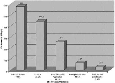 Figure 2-3 Measured performance of applications on the 644-processor Cray T3E at the National Energy Research Scientific-Computing Center (NERSC). This figure shows the sensitivity of performance to specific applications. These performance curves show that the Linpack benchmark does not represent a general application environment accurately. The average application at NERSC performs at 11.6% of the theoretical peak. In U.S. climate-modeling centers a 10% performance goal is often set. Thus, to achieve sustained speeds of 10–100 Tflops, peak speeds of 100–1000 Tflops would be required. Sustained-to-peak ratios in excess of 33% are common on the Japanese VPP computers, which coupled with their much higher single processor speed leads to a performance-usability gap between MPP and VPP systems. |
TABLE 2-1 Serial and Parallel Performance of Models on Microprocessor and Vector Processor Systems
|
Computer type |
VPP |
SMP |
|
Sustained rate [Gflops/PE] |
∼ 1 |
∼ 0.05 |
|
Ttot(1) [hours] |
278 |
5556 |
|
Speed-up factor required = S(N, fs) |
23 |
463 |
|
N required if fs = 0.01 |
30 |
no solution |
|
Efficiency = S(N, fs=0.01)/N |
77% |
— |
|
N required if fs = 0.001 |
24 |
850 |
|
Efficiency = S(N, fs=0.001)/N |
96% |
54% |
cheaper, slower parts than a network to support 24–32 vector processors. As pointed out earlier, the large size of the network and the slowness of the network components conspire to reduce further the effectiveness of SMP clusters compared to VPPs.
Strictly speaking, Amdahl's Law can be applied rigorously only to systems in which a single processor has uniform access to all of the memory required to hold the same problem that is run on N processors. This is the case in traditional shared-memory VPPs like the Cray C90 and NEC SX-4, but it is not so in distributed-memory SMPs like the SGI Origin 2000 or the IBM SP. The latter have non-uniform (much slower) access to memory that resides on other nodes, compared to the access rate to memory on the processor's node, resulting in further slow down.
Another major inefficiency that affects codes on parallel computers is load imbalance: different processors have differing amounts of work to do, so that some sit idle while others are overburdened. This is a problem for atmospheric General Circulation Models (GCM) that arises from differing amounts of work over land and ocean in the day and night hemispheres and at different latitudes. In ocean models land points must be eliminated from the computational domain to the greatest extent possible so that processors do not sit idle. If the component models of a coupled model run in parallel, load imbalance can cause components to sit idle while waiting to receive information from another component.
|
Box 2-6 The Load Balancing Issue To achieve good performance with massively parallel computers each processor should be given an equal “load” of the total computational work. If there is a load imbalance where one or more processors compute significantly more of the load, then a significant fraction of the processors may lay idle during a given computation, reducing both efficiency and overall performance. |
These facts regarding parallel scalability are reflected in the performance achieved for important, widely used climate and weather codes. Table 2-2 summarizes the performance of several such codes, including
TABLE 2-2 Comparison of Capacity and Capability Between Vector Processors and Massively Parallel Processors in Supercomputing
|
Model |
Single Processor (serial execution) |
Multiple Processor (parallel execution) |
||
|
Processor type |
Micro |
Vector |
Micro |
Vector |
|
IFS (ECMWF) [1] |
1CRI 2T3E 3600 Mhz 41 PE 52.14 fdpd 6N/A |
1Fujitsu 2VPP 5000 39.6 Gflops peak 41 PE 5102.5 fdpd 6N/A 748 |
1CRI 2T3E 3600 Mhz 41408 PEs 51800 fdpd 6N/A |
1Fujitsu 2VPP 5000 39.6 Gflops peak 498 PEs 57100 fdpd 6N/A 756 |
|
MC2 (Canada) [2] |
1SGI 2Origin 2000 3250 Mhz, 4 MB 41 PE 580 Mflops 616% |
1NEC 2SX-5 38 Gflops peak 41 PE 53500 Mflops 644% 744 |
1SGI 2Origin 2000 3250 Mhz, 4 MB 412 PEs 5840 Mflops 614% |
1NEC 2SX-5 38 Gflops peak 428 PEs 595200 Mflops 642% 748 |
|
GME/LM (Germany) [3] |
1CRI 2T3E 3600 Mhz 41 PE 560 Mflops 65% |
1Fujitsu 2VP 5000 39.6 GF/s peak 41 PE 53000 Mflops 631% 750 |
1CRI 2T3E 3600 Mhz 41200 PEs 5? 6? |
1Fujitsu 2VP 5000 39.6 Gflops peak 4? 5? 6? 750 |
|
MM5 (US) [4] |
1Compaq 2Alpha Server 3667 Mhz 41 PE 5360 Mflops 627% |
1Fufitsu 2VP 5000 39.6 Gflops peak 41 PE 52156 Mflops 622% 76 |
1Compaq 2Alpha Server 3667 Mhz 4512 PEs 545317 Mflops 66.6% |
1Fujitsu 2VP 5000 39.6 Gflops peak 420 PE 527884 Mflops 615% 716 |
|
The entries in the table are: 1manufacturer; 2model; 3processor characteristics; 4number of processing elements (PEs); 5sustained rate obtained with model (units are either “fdpd” = forecast days per day, or “Mflops”), 6sustained rate as % of peak performance rate; and 7ratio of sustained rates per processor of vector processor(s) to microprocessor(s). [1] Personal Communication, David Dent, ECMWF, Great Britain. [2] Personal Communication, Steve Thomas, NCAR, USA. Also see: M. Desgagne, S. Thomas, M. Valin, “The Performance of MC2 and the ECMWF IFS Forecast Model on the Fujitsu VPP700 and NEC SX-4M”, to appear in the Journal of Scientific Programming. [3] Personal Communication, Ulrich Schaettler, Deutscher Wetterdienst, Germany. Also see the paper: D. Majewski, et al., The Global Icosahedral-Hexagonal Grid Point Model (GME) Operational Version and High-Resolution Tests, ECMWF Workshop on Global Modeling, 2000. [4] Personal Communication, John Michalakes, NCAR, USA. Also see the web site: http://www.mmm.ucar.edu/mm5/mpp/helpdesk and the paper: J. Michalakes, “The Same Source Parallel MM5” to appear in the Journal of Scientific Programming. |
||||
IFS, MC2, MM5, and LM/GME (A more detailed description of each code is provided in Appendix I). Each code has a best microprocessor and vector performance achieved for both serial and parallel execution. We then compare them using the ratio of the sustained performance per processor between vector and microprocessor machines for both serial and parallel execution. The implications of the different performance characteristics will be explored in the following sections.


