Progress in Improving Project Management at the Department of Energy: 2001 Assessment (2001)

The standard EVMS reporting quantities, cumulative through reporting period t (typically in months), are defined as follows:

To apply control charting methods,¹ it is necessary to consider the earned value quantities in a single reporting period t, written as:

The cumulative and incremental definitions are linked by the following:

That is, acwp(t) is the actual cost of work performed in the time period t, whereas ACWP(t) is the cumulative actual cost of the work performed from the beginning of the project through time period t. The time period is the reporting period, usually a month.

Due to random fluctuations in project conditions, the dimensionless indices spi(t) and cpi(t) will vary. These statistical variations are typically assumed, for convenience, to be drawn from normal distributions, with some defined means and standard deviations. If the project is in a state of statistical control, these means and variances will be stable. The mean values of spi(t) and cpi(t) should be 1.0 (greater than 1.0 is better; less is worse) and the variances of both should be acceptably small. Zero variances, which would indicate exceptional quality of project planning and control, are unlikely to occur. The objective of the analysis is to determine whether a project has gone out of statistical control, which means that either the mean of spi(t) or cpi(t) is changing or the variance is changing, or both. And if a project is going out of control, this may mean that the project will go over schedule or over budget in the future.

To evaluate whether a change is occurring in the mean (the measure of central tendency) of spi(t), one should first establish the average value and the standard deviation based on historical data from projects that are considered to have been under control and good performers. Then, upper and lower natural process limits (UNPL and LNPL), which are conventionally three standard deviations above and below the mean, are derived. This usage is the source for the well-known six-sigma limits in statistical process control charting (one sigma is the standard deviation). Then, the probability that the measured spi(t) will be below the three-sigma LNPL (based on the normal distribution) owing to statistical fluctuations alone is 0.0013, and the probability that spi(t) will be above the UNPL is also 0.0013. That is, if the measured spi(t) is below the LNPL, this indicates that the process may be going out of control, as the probability that this value would occur with the process in control is only about 1/1,000. More specifically, if management were to follow up on every value of spi(t) below the LNPL to investigate a possible adverse change in the process, management would be wrong only once in a thousand times.

As a simple indicator of dispersion or variability, control charting methods often use the period-to-period range, which is the absolute magnitude of the

difference between the current period value and that in the previous period—for example:

The mean and the variance for the range can be determined by statistical methods,² and the upper control limit and the lower control limit for the range established as the mean plus or minus three standard deviations, as before. Then, if spi range(t) is observed above the upper control limit, there is only one chance in a thousand that this would occur through random fluctuation if the process is in control, and it is more likely due to a change in the variability of the process.

Note that the mean of the process, E[spi(t)], could be changing with no change in the variance, or vice versa. Also, some changes are beneficial: a decrease in E[spi(t)] may indicate that the project will fall behind schedule, but an increase in E[spi(t)] is favorable. Similarly, a reduction in the standard deviation of spi(t) means that the project is under tighter control, whereas an increase in the standard deviation may be indicative of future problems.

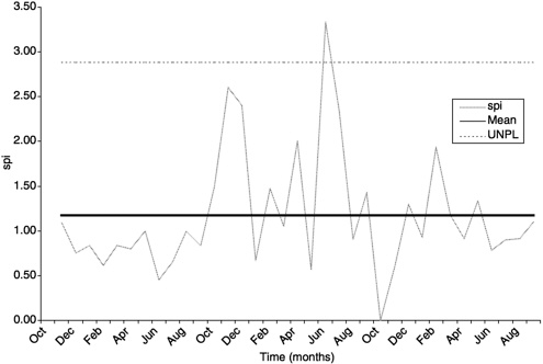
Figure E-1 shows the incremental (monthly) values for spi(t) for the Tritium Extraction Facility, along with the mean and the natural process limits. These are the same EVMS data as shown in Figure 5–1 but on an incremental, monthly basis. In this case, the process limits were computed using this project only, so the plot merely indicates that the project is staying within itself. As shown in the earned value plot (Figure 5–1), this project is close to schedule and budget at the last shown reporting date, so presumably is not in trouble, and the plot of monthly spi(t) corroborates this. A project in trouble would show values outside the process limits or other indications of changing conditions.

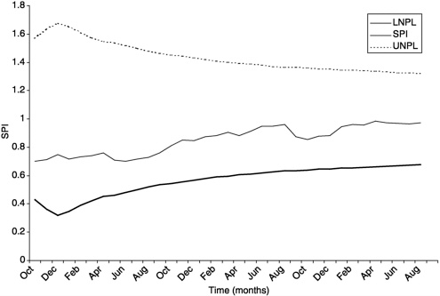
The same information can be shown on a cumulative or running SPI(t) plot, if preferred, as in Figure E-2. Here, the six-sigma band between the upper and lower process limits narrows with time, to compensate for the inertial effect of past history—that is, as t increases, a major change in spi(t) results in a smaller change in the cumulative SPI(t). Figure E-2 shows that although SPI(t) starts out below 1.0, it is still in the six-sigma band, so both plots give the same indication: the fluctuations (typically called “variances,” but here the term “variance” is always used in the statistical sense, to mean “square of the standard deviation”) are within the natural process limits, so no management attention is required.

Of course, the six-sigma process limits are simply points on the normal probability distribution and by themselves say nothing about quality. To use the measured data for quality control, one must determine the upper and lower specification limits (USL and LSL), the band of acceptable performance—that is, the

band in which management specifies that the values should lie. Then, if LSL < LNPL < UNPL < USL, the process lies within the specification requirements, quality is acceptable (this is six-sigma quality), and management should be happy. If LNPL < LSL < USL < UNPL, the process lies outside the specification requirements, quality is unacceptable, and management should be taking action.

A comparable metric is the capability index, Cp, which may be defined as Cp =(USL–LSL)/(six-sigma). If Cp < 1, the process is not very capable; that is, it cannot produce acceptable quality.

Of course, one does not have to place the limits at three standard deviations above and below the mean. Generally, six-sigma quality is regarded as excellent quality. Not every process is excellent, and this includes the DOE project management process. For example, consider the Tritium Extraction Facility plots in Figures E-1 and E-2. In these, the process limits were computed from the variations in this single project. No attempt is made here to set the specification limits, but the values are so highly variable (i.e., the standard deviation is so high) that the six-sigma process limits are extremely broad. It is very likely that acceptable specification limits would lie well inside this band, meaning that the variability in this project may be consistent but is too high to be considered good quality.

Figures E-1 and E-2 relate to the schedule performance index spi(t) and SPI(t), but identical arguments apply to the cost performance index cpi(t) and CPI(t).

In addition, there are many other variables that could provide management with indicators of potential project problems. One example would be change orders across all projects in one PSO; the Phase II report expressed the opinion that changes on DOE projects were out of control, and charting changes over time would indicate whether DOE is improving.

From the perspective of OECM, there are a sufficient number of projects in DOE to provide the statistical basis for applying six-sigma control charting as a filter, to identify projects that may be trending out of control. In fact, each of the three major Program Offices has enough projects to do this separately. The value of the statistical charting method is that it would put the evaluation of projects throughout the complex on a consistent, scientific, objective basis. There is, of course, vastly more about interpretation of control charts than is discussed here (see Breyfogle, for example, or any good textbook on statistical process control); the necessary computations are not presented here, but they are easily performed automatically on a computer.

It should be reemphasized that, for any charting and analysis to occur, the values must be measured and reported. That is, if there is ever to be any improvement, the project reporting system must be designed to support the needs of analysis.

Statistical studies have shown that the use of the cumulative CPI(t) provides an efficient estimator for the estimated cost at completion (ECAC). That is, from

CPI(t)=BCWP(t)/ACWP(t)

one derives

ECAC=BAC/CPI(t)

where BAC=budget at completion. There is no corresponding equation for the estimated date at completion (EDAC) in general use. However, there are methods for estimating EDAC from BCWS(t) and BCWP(t)—for example, linear and nonlinear regression—that could be evaluated for use in PARS. Even regression is easily performed by computer. Obviously, any forecast of EDAC and ECAC depends on accurate reporting without rebaselining. If a project is continually rebaselined such that CPI(t)=1, the above equation will always give ECAC= BAC.