Technology Development for Army Unmanned Ground Vehicles (2002)

This appendix provides details on the progress toward achieving autonomous A-to-B mobility through advances in the enabling technology areas of perception, navigation, planning, behaviors, and learning. Except for exclusively teleoperated applications, Army unmanned ground vehicles (UGVs) must be able to move from point A to point B with minimal or no intervention by a human operator. For the foreseeable future, however, soldiers will be needed to control UGVs, even on the battlefield, and the issue will be the number of soldiers required to support UGV operations. The more autonomous the vehicle, the lower the demands on the operator and the higher the degree to which UGVs effectively augment ground forces.

A UGV must be able to use data from on-board sensors, to plan and follow a path¹ through its environment, detecting and avoiding obstacles as required. Perception is a process by which data from sensors are used to develop a representation of the world around the UGV, a world model, sufficient for taking those actions necessary for the UGV to achieve its goals. “Perception is finding out, or coming to know, what the world is like through sensing perception extracts from the sensory input, the information necessary for an intelligent system to understand its situation in the environment so as to act appropriately and respond effectively—to unexpected events in the world” (Albus and Meystel, 2001). The goal of perception is to relate features in the sensor data to those features of the real world that are sufficient, both for the moment-to-moment control of the vehicle and for planning and replanning. Perception by machine² is an immensely difficult task in general, and machine perception to meet the needs of a UGV for autonomous mobility is particularly so.

The actions required by a UGV to carry out an A-to-B traverse take place in a perceptually complex environment. It can be assumed that Future Combat Systems (FCS) UGVs will be required to operate in any weather (rain, fog, snow) during the day or night, potentially in the presence of dust or battlefield obscurants and in conjunction with friendly forces likely opposed by an enemy force. The UGV must be able to avoid positive obstacles, such as rocks or trees, and negative obstacles, such as ditches. It must avoid deep mud or swampy regions, where it could be immobilized and must traverse slopes in a stable manner so that it will not turn over. The move from A to B can take place in different terrains and vegetation backgrounds (e.g., desert with rocks and cactus, woodland with varying canopy densities, scrub grassland, on a paved road with sharply defined edges, in an urban area) with different kinds and sizes of obstacles to avoid (rocks in the open, fallen trees masked by grass, collapsed masonry in a street) and in the presence of other features that have tactical significance (e.g., clumps of grass or bushes, tree lines, or ridge crests that could provide cover). Each of these environments imposes its own set of demands on the perception

system, modified additionally by such factors as level of illumination, visibility, and surrounding activity. To do the A-to-B traverse, the robotic vehicle requires perception for the moment-to-moment control of the vehicle and for planning a local trajectory consistent with the global path, detecting, locating, measuring, and classifying any objects³ that may be on the planned global path so the robot can move to avoid or stop.⁴ In addition to obstacles it must detect such features as a road edge, if the path is along a road, or features indicating a more easily traversed or otherwise preferred local trajectory if it is operating off-road.

The perception system must also be able to detect, classify, and locate a variety of natural and manmade features to confirm or refine the UGV’s internal estimate of its location (recognize landmarks); to validate assumptions made by the global path planner prior to initiation of the traverse (e.g., whether a region through which the planned path lies is traversable); and to gather information essential for path replanning (e.g., identify potential mobility corridors) and for use in tactical behaviors⁵ (e.g., upon reaching B, find and move to a suitable site for an observation post, or move to cover).

Specific perception system objectives for road following, following a planned path cross-country, and obstacle avoidance are derived from the required vehicle speed and the characteristics of the assumed operating environment (e.g., obstacle density, visibility, illumination [day/night], weather [affects visibility and illumination but may also alter feature appearance]). How fast the UGV may need to go for tactical reasons will establish performance targets for road following and cross-country mobility. The principal consideration in road following is the ability to detect and track such features as road edges, which define the road, at the required speed and to detect obstacles at that speed in time to stop or avoid. For the cross-country case, perception system performance will be largely determined by the size of obstacles the vehicle must avoid as a function of speed and the distance ahead those obstacles must be detected in order to stop or turn.

Obstacle detection is complicated by the diversity of the environments in which the obstacles are embedded and by the variety of obstacles themselves. An obstacle is any feature that is a barrier to mobility and could be an isolated object, a slope that could cause a vehicle to roll over, or deep mud. The classification of a feature as an obstacle is therefore dependent both on the mobility characteristics of the vehicle and its path. Obstacle detection has primarily been based on geometric criteria that often fail to differentiate between traversable and intraversable objects or features. This failure can lead to seemingly curious behavior when, for example, a vehicle in an open field with scattered clumps of grass adopts an erratic path as it avoids each clump. The use of more sophisticated criteria to classify objects (for example, by material type) is a relatively recent development and still the subject of research. Table C-1 suggests the scope of obstacles, environments, and other perceptual challenges.

The state of the art is based primarily on recent research carried out as part of the Army Demo III project, 1998–2002 (e.g., Bornstein et al., 2001); the Defense Advanced Research Projects Agency (DARPA) PerceptOR (Perception Off-Road) project (Fish, 2001) and other research supported by DARPA; the U.S. Department of Transportation, Intelligent Transportation Systems Program (e.g., Masaki, 1998); and through initiatives in Europe, mostly in Germany (e.g., Franke et al., 1998). The foundation for much of the current research was provided by the DARPA Autonomous Land Vehicle (ALV) project, 1984–1989 (Olin and Tseng, 1991) and the DARPA/Army/Office of the Secretary of Defense (OSD) Demo II project, 1992–1996 (Firschein and Strat, 1997). The discussion to follow is divided into three parts: road following, off-road mobility, and sensors, algorithms, and computation.

Army mission profiles show that a significant percentage of movement (70 to 85 percent) is planned for primary or secondary roads. Future robotic systems will presumably have similar mission profiles with significant on-road components. Driving is a complex behavior incorporating many skills. The essential but not sufficient driving skills for on-road mobility are road following or lane tracking and obstacle avoidance (other vehicles and static objects).

On-road mobility has been demonstrated in three environments: (1) on the open road (highways and freeways), (2) in urban “stop and go” setting with substantial structure and (3) following dirt roads, jeep tracks, paths, and trails in less structured environments from rural to undeveloped terrain. In the first two cases there is likely substantial a priori information available, but less in less structured environments. In all on-road environments, the perception system

must at a minimum detect and track a lane to provide an input for lateral or lane-steering control (road following); detect and track other vehicles either in the lane or oncoming, to control speed or lateral position; and detect static obstacles in time to stop or avoid them.⁶ In the urban environment, in particular, a vehicle must also navigate intersections, detect pedestrians, and detect and recognize traffic signals and signage.

Substantial research has been carried out using perception to detect and track lanes on structured, open roads (i.e., highways and freeways with known geometries, such as widths and radii of curvature), prominent lane markings, and well-delineated edges (for examples see Bertozzi and Broggi (1997); Masaki (1998); Sato and Cipolla (1996); Pomerleau and Jochem (1996)). Most of the approaches used have been model driven. Knowledge of the road’s geometry and other properties is used with features detected by the perception system (e.g., line segments) to define the lane and determine the vehicle’s position within it. Sensors used for lane detection and tracking include stereo and monocular color video cameras and forward looking infrared radar (FLIR) for operation at night or under conditions limiting visibility. A representative capability is described in Pomerleau and Jochem (1996). It was called RALPH (rapidly adapting lateral position handler) and used a single video camera. RALPH was independent of particular features as long as the features ran parallel to the road. It could use lane markings, patterns of oil drops, road wear patterns, or road edges. The features did not need to be at any particular position relative to the road and did not need distinct boundaries. A set of features was used to construct a template. Comparisons of current conditions with the template established the vehicle’s lateral position and generated steering commands. This system was used in the “No Hands Across America” experiment in 1995,

when RALPH drove a commercial van 2,796 miles out of 2,850 miles at speeds up to 60 mph.⁷ It worked well at night, at sunset, during rainstorms, and on roads that were poorly marked or with no visible lane markings but with features such as oil drops on the road or pavement wear that could be used to locate the lane. The most challenging situation was when the road was partially obscured by other vehicles. In some of those cases RALPH was able to lock on the vehicle ahead and follow it. When the following vehicle was close to the vehicle ahead of it the prominent vertical edges of that vehicle dominated the scene and RALPH treated it as a lane. RALPH could self-adapt to changing situations by looking far ahead of the vehicle (70 to 100 meters) and using the appearance of the road at that distance to construct a new template. RALPH made assumptions about road curvature between foreground and background to project what the new template should look like when the vehicle was centered in its lane. Comparison between the current image, the current template, and the look-ahead template allowed RALPH to decide if the situation had changed enough to warrant switching to the look-ahead template. RALPH was integrated with obstacle avoidance behavior⁸ as part of a demonstration under the U.S. Department of Transportation’s Intelligent Transportation Systems program.

Some of the preceding approaches for lane detection and tracking would work in urban “stop and go” environments; some would not. Parked cars or traffic in the urban environment may intermittently occlude many of the cues used to locate the lane in an open-road environment. Operation in the urban environment is a complex problem; only limited research has been done thus far, most by Franke and his colleagues (Franke et al., 1998). The procedure for urban lane detection and tracking used by Franke et al. was data or feature driven. A geometrical model cannot be easily developed because of the complexity of road topology. A given scene may be an unpredictable, complex combination of curbs, stop lines, pedestrian crossings, and other markings. Franke et al. (1998) first extracted edges and sorted them using specialized feature filters according to such attributes as length, orientation, parallelism, and colinearity. Combinations were created using a rule set and provided to a polynomial classifier trained on example feature sets. The classifier categorized the features as curbs, road markings, or clutter. Vehicles and other objects detected thru stereovision were excluded from consideration as road structure.

Part of road following, particularly in an urban environment, is the detection and navigation of road junctions and intersections. This has not received much emphasis. Early work was done by Crisman (1990) and Kluge and Thorpe (1993). More recently Jochem and Pomerleau (1997) described an approach that used selective image transformations to adapt an existing lane features detector to a wide variety of intersection geometries. They reported successfully detecting each intersection branch in 33 of 35 Y and T intersections. In no case did they report a branch that was not present. This is probably state of the art. Their approach was also notable in its use of active camera control (active vision)⁹ to pan the camera and track the detected branch so the vehicle could drive onto it.

As the technology for following structured roads has matured, it has begun to attract serious commercial interest. Carnegie Mellon University (CMU) and AssistWare Technology (Jochem, 2001) have jointly developed the Safe TRAC vision-based lane tracking system under U.S. Department of Transportation (USDOT) funding. A derivative of the RALPH system, it uses a single video camera to measure the vehicle’s position in the lane and provides an alarm if the vehicle weaves or drifts. Intended to provide driver warning, it could, like RALPH, be used to control the vehicle. It has undergone 500,000 miles of on-road testing; operating effectively on over 97 percent of all combinations of highways and driving conditions encountered (day, night, rain, snow, various levels of marking quality) with a false alarm rate of one per eight hours of driving. See Jochem (2001) for details.

An optically guided bus system¹⁰ is scheduled to go into service in Las Vegas in 2003. The argument for its use is precision in lane keeping, allowing buses to use a lane that is typically five feet narrower than buses that rely on human drivers. The system, called CIVIS (Eisenberg, 2001), is produced in France by a joint venture of Renault and Fiat. It is already in use in two French cities.

Essentially no work has been done on the related problem of detecting roads embedded in a cross-country environment. This is important when a vehicle is navigating primarily cross-country but where part of the planned path is on a road segment, probably unstructured, that passes through the

terrain. A related gap exists in the ability to seamlessly switch between cross-country and road-following behaviors. These behaviors have for the most part been developed independently. To switch requires manual intervention by the operator.

Unstructured roads pose a challenge because many of the assumptions behind the approaches described above for structural roads may be invalid: The appearance of the road is likely to be highly variable, making tuning of sensors and algorithms difficult. There are generally no markings, although there may be linear features so a RALPH-like approach might work in some situations. Edges may not be distinct and will likely be discontinuous (e.g., portions of the road or track may be obscured by vegetation or the road may be washed out in places). Lane size and curvature may vary irregularly, as may slope. This suggests that a data-driven (versus model-driven) approach will likely be preferred. The roads may be rough and heavily rutted requiring the vehicle to slow. High crowns may become obstacles and must be measured. Mud is almost guaranteed to be a problem and must be detected.

Because of this variability, the approaches all contain some means for learning from example. Chaturvedi et al. (2001) used a Bayesian classifier to segment roads from background in color imagery. They worked exclusively in a tropical environment with rich color content. The roads were red mud with ill-defined and irregular edges of green vegetation. Variations in light were severe (harsh sun to deep shadows) and visibility was also affected intermittently by rain. Both of these conditions caused the edges to disappear at times. The lack of well-defined edge features motivated the use of color segmentation. They worked in the HIS (hue, intensity, saturation) color space because of the relative invariance of hue to shadows. They were able to successfully segment jungle roads at about 5 Hz under a variety of lighting and weather conditions. Although this specific approach is limited by the constraint that the road be red in color, it does suggest that color segmentation more broadly could be useful in the detection and following of unstructured roads. Because colors change under different illumination, the broad applicability of color segmentation will require finding either color properties that are relatively invariant in shadows or for highlighted surfaces or a means to recover an estimate of the color of the illumination from the scene.

RALPH was a purely reactive system. ROBIN had a deliberative component. Rosenblum (2000) described an improved version of the ROBIN neural-network-based system used in Demo II. This version was used for unstructured road following in the early part of the Demo III program and in other unrelated experiments. Unlike ALVINN, which used a three-layer, feed-forward neural network, ROBIN used a radial basis function (RBF) neural network. An advantage of RBFs is that they smoothly fill gaps in training examples and can be trained very rapidly. A second way that ROBIN differed from ALVINN (or other strictly neural-network solutions) was in the inclusion of a deliberative reasoning module. This monitored performance of the road-following module and could act to improve performance. For example, it could slow the vehicle to obtain multiple looks in an ambiguous situation, change the virtual camera view, or change the parameters used in image preprocessing. ROBIN was able to drive on secondary roads at 25 mph and on ill-defined roads and trails at 10 mph, during daytime, using pseudo black and white video derived from a color camera. Using a FLIR, ROBIN drove secondary roads at night at 15 mph and the ill-defined roads and trails at 10 mph. Rasmussen (2002) described a system that showed the potential of fused laser detection and ranging (LADAR) and color video data in road following. The data were coregistered in space and time. Height and smoothness (height variation in the local vicinity of a point) features were derived from the LADAR. A color histogram was calculated for each color image patch, as was texture. The assumptions were that roads should be locally smooth, be consistent in a mix of brown or gray colors, and exhibit more homogeneous texture than bordering vegetation. The feature data was fused in a three-layer neural-network classifier. The results showed the road was clearly segmented despite shadowing and changes in composition. Training individual neural networks by road type improved performance over a single network. Using data from both sensors produced substantially better performance than any single sensor. This work was done off-line. The approach is currently too computationally demanding for real-time application.

There has been much less research on following unstructured roads than on highways and freeways; systems are not as robust and problems are less well understood. Challenges include roads with sharp curves where the system may lose the road, steep slopes where the slope may be incorrectly classified as an obstacle, judging water depth if the road includes a stream crossing or standing water, and following roads that are defined by texture and context rather than color, changes in contrast, or three-dimensional geometry. Performance in rain is likely to be highly variable, depending on specifics of the road.

On-road detection includes static obstacles and detecting and tracking other vehicles. Williamson (1998) focused on static obstacles, used a stereo-based approach and could reliably detect objects 14 cm or taller out to distances of 110 meters using narrow field of view, long focal length lenses. He also demonstrated obstacle detection at night using the vehicle’s headlights. One obstacle was painted white and was 14 cm tall. It was detected at a range of about 100 meters using the high beams. A similar size black obstacle was detected at 60 meters. Williamson used a three-camera system to reduce the likelihood of false matches. Williamson worked in a structured road environment. There has been little com-

parable research to detect obstacles on unstructured roads, where for example, abrupt changes in slope may cause false positives with some algorithms. There has been no work specifically to detect on-road negative obstacles. Off-road work is applicable.

Franke et al. (1998) and others worked on vehicle detection and tracking. Franke et al. used a very efficient stereo algorithm that could work in real time; Dellaert and Thorpe (1998) used a two-dimensional approach that also worked in real time. Betke et al. (1996) used edge images to find distant cars. Their approach first did a coarse search to find regions that might contain cars and then did a fine-grained search and match on those regions. Beymer and Malik (1996) used a feature-based technique with such features as a portion of a bumper or prominent corners. They assumed that features that moved together should be grouped together and used Kalman filtering to track the feature groups. Giachetti et al. (1995) used optical flow for detecting and tracking vehicles. This does not work well without good texture and when there is large motion in the image sequence. They developed some multiscale and multiple window algorithms to address these problems. All the above were successful in detecting vehicles both in lane and as oncoming traffic.

Many of the techniques for on-road obstacle detection used video cameras as the sensor. This was driven in part by the desire to put inexpensive systems into private and commercial vehicles. They can be used at night with external illumination but do not work well in fog, smoke, or other situations where visibility is limited. Extensive work was done using FLIR and LADAR for off-road obstacle detection (to be described later) that was equally applicable to the detection of obstacles on road. They provided improved performance at night and under limited visibility but are expensive, and LADAR is range limited. Increasingly it was recognized that no one-sensor type no matter how clever the processing could do everything. Multiple sensor modalities would be required and their results combined to achieve robust obstacle detection under all weather conditions. Langer (1997) developed a system that combined data from a 77-GHz radar with data from a video camera. The radar was used to detect and locate other vehicles. Video provided to the RALPH road-following system sensed road geometry and was used to maintain lateral position. Road geometry information from RALPH was used for clutter rejection and to reduce the number of false positives from the radar. With the addition of radar data RALPH could also autonomously control speed, maintaining a safe driving distance from preceding vehicles. The system was able to track multiple vehicles successfully, both in-lane and in the opposing lane in a cluttered urban environment. Cars could be reliably detected at distances up to 180 meters and trucks up to 200 meters. Langer also detected people at 50 meters. Collision avoidance systems are beginning to find commercial applications (Jones, 2001). Based on radar (77 GHz), LADAR, or stereo from video cameras, these are part of the next generation of adaptive cruise control (ACC) systems, which will maintain a safe distance to the car ahead, braking or accelerating up to the speed preset by the driver.¹¹ Systems are being sold today by Toyota, Nissan, Jaguar, Mercedes-Benz, and Lexus. GM, Ford, and others plan ACC offerings this year or next. Fujitsu Ten Ltd., in Plymouth Michigan, is developing an ACC for stop-and-go driving. It fuses data from millimeter-wave radar and 640 × 480 stereo video cameras. This takes advantage of the ability of the radar to look far down the road and to provide a wide field of view for tracking cars in turns and using stereo to improve clutter rejection and reduce false alarms caused by stationary objects. So far, no organization has announced that they are developing a commercial system that combines adaptive cruise control and lane tracking.

If vehicles can be detected and tracked for collision avoidance, they also can be followed. Of note was the autonomous leader-follower capability demonstrated by Franke et al. (1998). Lead car speed was variable from a stop up to 12 m/s (43 km/h) and was accurately tracked by an autonomous follower vehicle while maintaining a safety distance of 10 meters. More recent perception-based leader-follower work (Bishop, 2000) was intended to enable close-headway convoying of trucks. This project, called CHAUFFEUR, used a pattern of lights on the preceding truck. The distortion of the pattern provided heading correction and the size of the pattern yielded distance. Leader-follower operation was demonstrated in Demo II (three vehicles that also demonstrated formation keeping) and Demo III (two vehicles). In both, the approach was GPS based and not perception based (i.e., the follower vehicle did not make use of perception to track the leader vehicle).

The detection of pedestrians remains a very difficult problem, particularly in cluttered scenes containing many people. Various approaches have been used; Franke et al. (1998) used shape templates and characteristic walking patterns. For detection of walking they used both color clustering on monocular images in a combined color and feature position space and three-dimensional segmentation. Papageorgiou et al. (1998) used a trainable system. Features were encoded at different scales. They used these features to train a support vector machine (SVM) classifier. Without using motion they achieved an 80 percent detection rate with about 10^–5 false positive rate. The detection rate approached 100 percent for a false positive rate of 10^–3. These results were obtained in cluttered urban scenes containing multiple pedestrians at varying distances.

More recent projects include that of Zhao and Thorpe (2000) at Carnegie Mellon University, which used stereo-

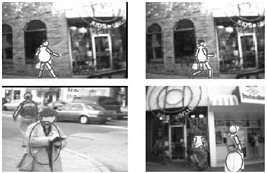
FIGURE C-1 Pedestrian detection. Courtesy of Chuck Thorpe, Carnegie Melon University Robotics Institute, and Liang Zhao, University of Maryland.

vision and a neural-network classifier (see Figure C-1); Broggi et al. (2000) at the University of Pavia, which combined stereovision with template matching for head and shoulder shapes; and Gavrila (2000) at Daimler-Chrysler, which also used stereovision and a time-delay neural network to search across successive frames for temporal pattern characteristics of human gaits. Gavrila (2001) estimates the state of the art at 90 percent to 95 percent detection rate with a false positive rate between 10^–3 and 10^–1.

Similar to vehicle detection and tracking, if a person can be detected and tracked for avoidance in an urban environment then a vehicle could also follow a person in open terrain.

The detection of signage and traffic signals is important in an urban environment. Signage consists of isolated traffic signs on poles and directional or warning symbols painted on the road surface. Franke et al. (1998) used a combination of color segmentation algorithms and gray-scale segmentation (to address situations where illumination or other factors affect color). Segmentation produced a region of interest that served as an input to a radial basis function classifier for signage and a three-layer neural network for traffic light recognition. For signs on roads and on poles they achieved recognition rates of 90 percent with 4 to 6 percent false positives. Recognition rates for traffic lights in a scene were above 90 percent with false positive rates less than 2 percent. Priese et al. (1995) also developed a system to locate and recognize traffic signs. It detected and recognized arrows on the road surface, speed-limit signs, and ideograms. For ideogram classification it used a neural-network-classifier to recognize 37 types of ideograms. They used some image transformation but assumed the signs were essentially viewed directly ahead. Peng and Bhanu (1999) used an adaptive approach to image segmentation in which 14 parameters in the Phoenix color-based segmentation algorithm were adapted to different conditions using reinforcement learning.¹² They were able to achieve about a 70 percent detection rate on stop signs under varying conditions where the sign was prominent in the image (i.e., centered and large). The rate dropped to about 50 percent in more difficult conditions when the sign was smaller and the surrounding clutter greater; note that without adaptation, the rate was about 4 percent. Peng and Bhanu (1999) showed how the performance of a well-understood general-purpose color segmentation algorithm could be improved by using learning to adapt it to changing conditions.¹³ In contrast, Franke et al. (1998) developed special purpose classifiers tailored to the sign detection problem.¹⁴ Meyers et al. (1999) considered

the problem of reading the characters on a sign viewed from an oblique perspective. They used a transform to rectify and deshear the image using parameters computed from the image itself. They achieved nearly 100-percent recognition accuracy up to azimuth angles of about 50 percent.

On-road mobility at a minimum requires perception for lane detection to provide lateral control of the vehicle (road following), perception for collision avoidance (i.e., detection and position and velocity estimation for vehicles in lane to maintain a safe distance through adaptive speed control), and perception for the detection of static obstacles.

Perception for lane detection and tracking for structured roads is at the product stage. About 500,000 miles of lane detection and tracking operation has been demonstrated on highways and freeways. Lanes can be tracked at human levels of driving speed performance (e.g., 65 mph) or better under a range of visibility conditions (day, night, rain) and for a variety of structured roads, but none of the systems can match the performance of an alert human driver using context and experience in addition to perception. Lane tracking may function in an advisory capacity providing warning to the driver that the vehicle is drifting out of the lane (Jochem, 2001) or it may be used to directly control steering (Eisenberg, 2001). There are other approaches that have not been as extensively tested; most (e.g., ALVINN, RALPH, ROBIN) have been used to control steering but only in research settings.

Detection and tracking in an urban environment are very difficult. Many of the perceptual clues used to navigate open roads may be available only intermittently because of traffic or parked cars, but these, in turn, can also serve to help define the road. Road following, intersection detection, and traffic avoidance cannot be done in any realistic situation. Signs and traffic signals can be segmented and read only if they conform to rigidly defined specifications and if they occupy a sufficiently large portion of the image. Pedestrian detection remains a problem. A high probability of detection (e.g., 98 percent) is accompanied by a high rate of false positives. This can be addressed by using multiple cues from different sensor modalities. Much research remains to be done.

Although the research has shown the ability of automated vehicles to follow structured roads with performance that appears similar to that of human drivers, there are many situations in which performance is not at the level of a human driver (e.g., complex interchanges, construction zones, driving on a snow-covered road [nearly impossible], driving into the sun at low sun angles, driving in precipitation [heavy rain, snow, or fog], and dust). The systems are almost exclusively sensor driven and are very limited in their ability to use all the context and experience available to a human driver to augment or interpret perceptual cues.

Road following assumes that the vehicle is on the road. A special case is detecting a road, particularly in a cross-country traverse, where part of the planned path may include a road segment. Work done on detecting intersections or forks in paved roads is applicable, but very little research has specifically addressed the detection of dirt roads or trails in open terrain. The level of performance on this task is essentially unknown.

A number of means, both active and passive, have been demonstrated for detecting and tracking other vehicles for collision avoidance, but only in research vehicles. Some have been used to control vehicle speed (e.g., Langer, 1997; Franke et al., 1998). Others have demonstrated the capacity to make the position and velocity estimates necessary to control vehicle speed but were not integrated into the control system. There have been limited demonstrations (e.g., Langer, 1997; Franke et al., 1998) that integrate both lane detection and tracking with collision avoidance for vehicle control. Avoidance of the moving targets represented by animals and pedestrians is another extremely challenging problem that has barely been touched by the research community.

The potential exists (stereovideo or stereo FLIR) to detect static, positive obstacles (e.g., 15 cm) on the road in time to avoid them or stop while traveling at high speed (e.g., 120 km/h with 120 meters look-ahead). A very narrow field of view is required, the approach is computationally demanding, and the sensors must be actively controlled. Radar has not been shown to detect small objects reliably (much less than car size) at these distances, and LADAR does not have the range or instantaneous field of view (IFOV).

Obstacle detection and avoidance behavior was integrated with lane-tracking behavior for vehicle control in the ALV program (see Appendix D) for Demo II (ALVINN and color stereo) and for a Department of Transportation demonstration (RALPH and color stereo); however, these demonstrations were staged under conditions much less demanding than real-world operations.

The existing technology is extremely poor at reliably detecting road obstacles smaller than vehicles in time to stop or avoid them. This is an inherently very difficult problem that no existing sensor or perception technology can address adequately. For example, an object 30 cm³ in size could cause serious problems if struck by a vehicle. A vehicle traveling at highway speed (30 m/s) would need to detect this object at greater than 100 meters to respond in time.

The reported research on reading road markings and road signs represents an extremely primitive capability at this time. It depends on those markings and signs being very carefully placed and designed, and none of the systems can deal with imperfect conditions on either. Even under good conditions, the error rate remains significant for these functions.

A variety of sensors can be used in various combinations for on-road mobility, depending on specific require-

ments. These include 77-GHz radar for long-range obstacle and vehicle detection and for use under low-visibility conditions; stereo color video or FLIR for lane following, vehicle and obstacle detection, and longer-range pedestrian detection; and LADAR or light-stripers for rapid, close-in collision avoidance, curb detection, and pedestrian detection.

Considerable effort is being invested within the automotive industry and related transportation organizations to develop systems that will enhance driving safety, assist drivers in controlling their vehicles, and eventually automate driving. These activities, which are international in scope, offer the potential for technology spin-offs that could eventually benefit the Army’s UGVs by lowering costs and accelerating the availability of components and subsystems. These include sensors, actuators, and software.

Autonomous off-road navigation requires that the vehicle characterize the terrain as necessary to plan a safe path through it and detect and identify features that are required by tactical behaviors. Characterization of the terrain includes describing three-dimensional terrain geometry, terrain cover, and detecting and classifying features that may be obstacles, including rough or muddy terrain, steep slopes and standing water as well as such features as rocks, trees, and ditches.

Terrain characterization has been variously demonstrated beginning with the ALV program but always in known environments and generally in daytime, under good weather conditions. Performance has continued to improve up to the present but measurement of performance in unknown environments¹⁵ and under a range of environmental conditions is still lacking. Most recent work was also done in daylight, during good weather. The DARPA PerceptOR program is addressing performance measurement in unknown terrain, all weather, day, and night.

Most of the research on perception for terrain characterization was in support of the Demo III and PerceptOR programs. The vehicles for Demo III were XUVs (experimental unmanned vehicles). These weighed about 3,400 pounds, had full-time, four-wheel drive and mobility characteristics essentially equivalent to a high-mobility multi-purpose wheeled vehicle (HMMWV) (Figure C-2 shows the XUV and PerceptOR¹⁶). Experiments were carried out both on XUVs and HMMWVs. The sensors used on the Demo III XUVs were stereo, color video cameras (640 × 480), stereo FLIR cameras (3-5, 320 × 256, cooled, 2-msec integration time), and a LADAR (180 × 32 at 20 Hz, 50-meter maximum range, 20-meter best performance, 7-cm-range resolution, and 9-mrad angular resolution [22° elevation, 90° azimuth]). Foliage penetration (1.5 GHz) and obstacle avoidance (77 GHz) radars were planned but have not yet been integrated. Stereo depth maps, including processing for limited terrain classification, were produced at 4 Hz.

Descriptions of how data from the XUV sensors and from the perception system were used to control the vehicle are given in Coombs et al. (2000) and Murphy et al. (2000). They reported cross-country speeds of up to 35 km/h in benign terrain: “rolling grass-covered meadows where the only obstacles were large trees and shrubs.” The conditions were daylight and in good weather. The vehicle they used was an HMMWV. They used a LADAR (128 × 64 pixels) operating at 1 Hz, detected large obstacles out to 40–50 meters, and concluded that this update rate, plus processing and planning latencies of about one second, limited the speed. Note that the XUV LADAR operates at 20 Hz. The vehicle control software (obstacle detection, cartographer, planner, reactive controller) was ported to the XUV.

Shoemaker and Bornstein (2000) reported that the Demo III Alpha experiments at Aberdeen, Md. (September 1999) used stereo obstacle detection at six or less frames per second. Using only geometric criteria, clumps of high grass were classified as obstacles and avoided. Bornstein et al. (2001) noted that the vehicle did not meet the 10-mph off-road goal, was not able to reliably detect negative obstacles, and had only limited capability in darkness. In October 2000, the Demo III Bravo experiments were held at Ft. Knox, Ky. LADAR was integrated into the vehicle for obstacle detection. Stereo obstacle detection performance was improved for both positive and negative obstacles. The vehicle still had difficulty with tall grass, in this case confusing the tops of the grass with the ground plane and causing the vehicle to avoid open, clear terrain and confusing it with a drop-off. The range limitation of the LADAR led to cul-de-sac situations where, for example, it could not see breaks in tree lines (Bornstein et al., 2001).

In demonstrations at Ft. Indiantown Gap, Pa., Murphy et al. (2002) reported that the XUVs were able to navigate

Murphy et al. (2002) noted that a major limitation was the limited range and resolution of the sensors, particularly the

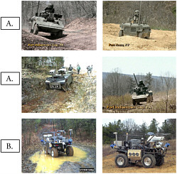
FIGURE C-2 Demo III vehicle and PerceptOR vehicle. Rows A courtesy of Jon Bornstein, U.S. Army Research Laboratory; Row B courtesy of John Spofford, SAIC.

LADAR, which could not reliably image the ground more than 20 meters ahead and had an angular resolution of about 9 mrad or about 0.5 degree.¹⁷ (By comparison, the human eye has a foveal resolution of about 0.3 mrad.) Murphy et al. suggested that the LADAR was the primary sensor used for obstacle detection. That is, without the LADAR the demonstrations would not have succeeded or performance would have been reduced substantially. Why stereo did not feature more prominently was not discussed.

Members of the committee observed the Demo III XUVs at Ft. Indiantown Gap in November 2001. The demonstrations confirmed reliance on LADAR and the fact that the XUVs pushed through brush with prior knowledge that no obstacles were concealed in the brush. The committee observed that the vehicles on occasion confused steep slopes that were within its performance range with intraversable terrain requiring operator intervention (see Figure C-3). The committee also confirmed the Murphy et al. observation about limited field of view after observing one of the vehicles get trapped in a cul-de-sac. On other occasions the committee noted that the vehicles would stop, or stop and backup, with operator intervention required to reestablish autonomous operation. The problem was dust affecting the LADAR performance. A dust cloud looked like a wall or a dense field of obstacles through which the planner could not find a safe path. Possible solutions include additional sensors, active vision, and algorithms that use last-pulse processing. Reliance on a single sensor is risky.

In related research the PRIMUS German research project reported cross-country speeds of 10 km/h to 25 km/h

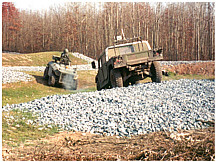
FIGURE C-3 Perception of traversable slope as an object. Courtesy of Clint Kelley, SAIC.

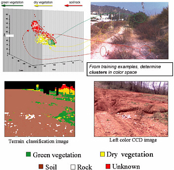
FIGURE C-4 Color-based terrain classification. Courtesy of Larry Matthies, Jet Propulsion Laboratory.

in open terrain (Schwartz, 2000). The project used a small tracked vehicle with good cross-country mobility. Obstacles were less of a problem than with a comparably sized wheeled vehicle. Obstacle detection was done with a Dornier 4-Hz LADAR (129 × 64, 60° × 30°) on a stabilized pan and tilt mount. A monocular color camera was used for contour or edge following. Durrant-Whyte (2001) reported cross-country speeds of 30 km/h over 20-km traverses also using LADAR.

Driving through dense brush, even knowing there are no hidden obstacles, is difficult. The perception system must assess the density of the surrounding brush to determine if the vehicle can push through or must detour. The Demo III system counted the number of range points in a LADAR voxel to estimate vegetation density. If the count was less than a threshold number, the vegetation was assumed to be penetrable. The assumption in Demo III was that the range points were generated by returns from vegetation; the system did not do classification. A fast statistical approach for analyzing LADAR data was described in Macedo et al. (2001) to classify terrain cover and to detect obstacles partially occluded by grass. They found statistically significant differences in the measures used between grass, and rocks partially occluded by grass. Castãno et al. (2002) described a classification approach using texture analysis of color video and FLIR images. The data were collected by the XUV operating at Ft. Knox. They classified a scene into the categories of soil, trees, bushes, grass, and sky. They obtained texture measurements from a bank of 12 spatial filters at different scales and orientation. The measurements were combined in both maximum likelihood and histogram-based classifiers. Classification accuracy (percent correct) during the day with the color data was between 74 percent and 99 percent, depending on the category, and at night with the FLIR data it was about the same: between 77 percent and 99 percent. Figure C-4 shows the process and typical results. The results were obtained off-line because of computational requirements. Bellutta et al. (2000) described stereo-based obstacle detection and color-based terrain cover classification using color and FLIR cameras. Potential obstacles were detected

using geometric analysis and then a Bayesian classifier was used to assign a material class to the object. Depth maps were produced at 6 Hz on a 320 × 240 image. A rule-based system could then be used to combine information on geometry and material type to assess traversability. A unique aspect of their approach was the use of active vision to point the narrow field-of-view stereo cameras. The cameras were pointed at the path the vehicle was currently commanded to follow with look-ahead distance determined by the vehicle’s speed. They demonstrated the system on an HMMWV. The classification results matched ground truth. The active vision software has not yet been ported to the Demo III XUV.

As part of the PerceptOR program, Matthies (2002) experimented with RGB (red, green, blue), near-infrared, and multiband FLIR imagery for terrain classification. He concluded that near-infrared (nonthermal, two-bands 0.65 µm and 0.80 µm) was more reliable and less affected by variable illumination than RGB, that two to three bands of thermal infrared (IR) in the range from 2 µm to 12 µm showed promise for discriminating vegetation from other material at night, and that texture analysis of thermal IR was very promising for discriminating vegetation from soil. This was the first work on possible means to characterize terrain cover at night.

In separate related research, Bhanu et al. (1997) used 12 spectral bands over the range from 0.44 µm to 1.4 µm to classify terrain. They used a hierarchical classification scheme with which regions in the scene were first labeled: road, field, forest, sky, and unknown. Field regions were then further subdivided into grass, scrub brushes, snowberries, and soil. They used a variety of means for classification, including texture and other feature extraction approaches at the lower level and knowledge based at the higher level for fusion and feature interpretation. They demonstrated the potential for multispectral terrain classification but only on a limited data set. The work was done off-line. Multispectral ground cover classification has long been a standard tool for remote sensing using overhead imaging. This potential should be exploited for ground vehicles.

Hong et al. (2000) and Manduchi (2002) both used data fusion for terrain classification. Hong et al. combined data from a LADAR and a single color camera. They described ways to detect standing water (puddles), signs, and roads and showed how fusion could improve performance over a single sensor. They fused the data in the world model using various heuristics, which also supported the fusion of information over time. Manduchi used a Bayesian classifier to fuse a set of local features statistically. This work also suggested improved performance from fusion. The use of texture as a feature precluded real-time operation.

The evaluation and comparison of terrain classification approaches in particular are qualitative and imprecise because of a lack of adequate ground truth and common datasets.

Substantial work was done on obstacle detection. Matthies et al. (1998) described a systematic effort to evaluate the performance of stereovision with camouflage, concealment, and detection (CCD) cameras and FLIR cameras against putative Demo III requirements. They did a series of obstacle detection experiments with stereo data collected at different times of day and night, and with different size obstacles. They concluded from an analysis of the data that an object that subtended 10 vertical pixels¹⁸ could be reliably detected.¹⁹ Given this value, they calculated the fields of view for a sensor to detect obstacles at several look-ahead distances, each corresponding to a specific cross-country speed (e.g., Demo III at 35 km/h). They included assumptions about vehicle dynamics and processing latencies. The calculations showed that there was an inherent conflict between the narrow field of view required to place 10 pixels on an object for reliable detection and the total field of regard necessary to see all terrain into which the vehicle could steer. They concluded active vision was required.

Owens and Matthies (1999) compared cooled and uncooled FLIRs and image intensifiers for stereo-based detection of obstacles at night. They concluded that only cooled FLIRs would meet requirements. The integration time for uncooled FLIRs, about 15 m/sec, was too long for the required speeds (causing excessive motion blur that washed out features) and the image intensifiers did not have an adequate signal-to-noise ratio for stereo matching. The cooled FLIRs worked very well and provided adequate contrast even at thermal crossover.

More recent and extensive research on obstacle detection is described by Matthies (2002). Sensors used included color video, LADAR, radar, and FLIR (operating in three bands, near [2–2.6 µm], medium [3–5 µm], and long wavelengths [8–12 µm]). The conclusions were that state-of-the-art stereo is 320 × 240 at 10 Hz on a Pentium III and at 30 Hz with application-specific hardware. For positive obstacles, the use of 10 pixels as a minimum obstacle height for detection is a good assumption where vegetation does not obscure the obstacles. Required sensor angular field of view can then be calculated from speed requirements. For positive obstacles in vegetation, detection depends on the size of the obstacle and the density of the vegetation. Both LADAR and radar can detect positive obstacles on the order of 45 cm × 65 cm a few meters into tall grass, depending on the density of the grass. LADAR can detect objects in brush out to about 1 meter. Much more research is required to predict performance across a range of conditions. Unobscured negative obstacles could not be reliably detected more than 10–15 meters ahead of the vehicle (sensor height about 2 meters with angular resolution of about 2.5 mrad). Limited work was done on detecting thin objects (a metal pole about 1.5 meter high and 5 cm wide). Detection with stereo was dem-

FIGURE C-5 Tree-line detection. Courtesy of Larry Matthies, Jet Propulsion Laboratory.

onstrated at 5 meters but not at 9 meters. Parameters that affect detection of various classes of thin objects were identified. Additional research is needed to be able to model performance. Some work was done on obstacle detection in the presence of obscurants (natural and smokes). The conclusion was that the performance of MWIR (3-5 µm) should be adequate.

Detection of water remained a problem. Matthies (2002) described the use of ratios of colors (green to near infrared), texture analysis of color images (water has little texture), stereo (few matches from the water relative to the surround), LADAR (specular-no return), and polarization. All work to some degree under some situations. For example, if the water reflects sky, then texture works well; if it reflects surrounding trees, then texture provides misleading results. Depending on subsequent research, data fusion may provide the best solution. Green LADAR may be able to measure water depth ahead of the vehicle. Further research is required.

Matthies (2002) and Chang et al. (1999) reported the first work on detection of tactical features. Matthies demonstrated tree-line detection with stereo color imagery at 45 and 80 meters (see Figure C-5). Chang et al. described the use of LADAR to detect overhanging trees and other over-hanging features and an algorithm to classify them either as potentially providing cover (a vehicle can go beneath it) or as an obstacle (too low). In one example they were able to detect and classify trees as providing cover or not at a range of 45 meters. If the two were combined, the vehicle could follow a tree line and take cover as required. This capability must be extended well beyond 100 meters.

No quantitative standards metrics or procedures exist for assessing off-road UGV performance. It is difficult to know if progress is being made in off-road navigation and where deficiencies may exist. The assessment problem is exacerbated by the absence of statistically significant published test results reflecting different operating conditions. Emphasis has been placed on meeting demonstration objectives rather than conducting controlled tests. A goal should be data collection sufficient to develop predictive models.

Unlike road following, speed²⁰ as a metric to gauge progress in off-road mobility is incomplete and may be misleading. No meaningful comparisons can be made without knowing the environmental conditions, the details of the terrain, and, in particular, how much reliance was placed on prior knowledge to achieve demonstrated performance. While it is reasonable to assume that Demo III performance is better than Demo II, there is no way to know from published reports; there are too many uncontrolled variables. Many of the issues identified in the ALV and Demo II programs remain problems today, and many of the capabilities demonstrated in Demo III could be replicated with Demo II algorithms enabled by improved computation. Similarly, there is no way to know how close Demo III performance is to meeting putative FCS or other requirements, since specificity is lacking on both sides. No data exist for performance in an a priori unknown environment. The PerceptOR program is addressing this gap, but results will not be available for about 2 to 3 years.

Because of uncertainty about UGV performance, it is not possible to estimate vehicle operator workload, nor how many vehicle operators might be required for a given force. With statistically valid vehicle performance data, predictive models of UGV performance could be developed, and these issues could be addressed through simulation.

Subjective comparison of UGV cross-country performance with the performance of manned vehicles on comparable terrain suggests that cross-country capability is very

immature and limited. Published results and informal communications do not provide evidence that UGVs can drive off-road at speeds equal to those of manned vehicles. Although UGV speeds up to 35 km/h have been reported, the higher speeds have generally been achieved in known benign terrain and under conditions that did not challenge the perception system or the planner. During the ALV and Demo II experiments in similar benign terrain, manned HMMWVs were driven up to 60 km/h. In more challenging and unknown terrain, the top speeds for all vehicles would be lower but the differential likely greater. While off-road performance is limited by sensor range and resolution, it may also be limited by the approach taken. Driving autonomously on structured roads is essentially reactive; surprises are assumed to be unlikely and speeds can be high. Driving off-road, with its inherent uncertainty, is currently treated as a deliberative process, as if surprises are likely. Higher-resolution sensor data is used to continuously produce a detailed three-dimensional reconstruction of the terrain currently limited by sensor capabilities and the way sensors are employed to no farther than 20 to 40 meters ahead of the vehicle. Trajectories are planned within this region. This is unlike the process used by human drivers who look far ahead to roughly characterize terrain. They adjust speed based on expectations derived from experience and context, local terrain properties, and by using higher-resolution foveal vision to continuously test predictions, particularly along the planned path. A UGV could use the same process. Sensors with a wide field of view but lower resolution could look farther ahead. Macro-texture and other features detected at lower-resolution could be used to continuously assess terrain properties for terrain extending out some distance from the vehicle. At the same time, the lower resolution sensors and other data (e.g., the planned path) could be used to continuously cue higher-resolution sensors to examine local regions of interest. Both the predictions and the local data would be used to reactively control speed. This is analogous to road-following systems previously described that look far ahead and judge that the scene still looks like a road and that no obstacle appears to be in the lane ahead. If the terrain ahead is similar to the terrain on which the vehicle is currently driving or can be matched to terrain descriptions in memory using a process like case-based reasoning, then assumptions can be made about likely speeds and verified using active vision. There is predictability in terrain, not as much as on a structured road, but some. The trick is to learn to exploit it to achieve higher speeds.

In principle, LADAR-based perception should be relatively indifferent to illumination and should operate essentially the same in daylight or at night. FLIR also provides good nighttime performance. LADAR does not function well in the presence of obscurants. Radar and FLIR have potential depending on the specifics of the obscurant. There has not been any UGV system-level testing in bad weather or with obscurants, although experiments have been carried out with individual sensors. Much more research and system-level testing under realistic field conditions are required to characterize performance.

The heavy, almost exclusive, dependence of Demo III on an active sensor such as LADAR may be in conflict with tactical needs. Members of the technical staff at the Army NVESD told the committee that LADAR was “like a beacon” to appropriate sensors, making the UGV very easy to detect and vulnerable (U.S. Army, 2002). Strategies to automatically manage the use of active sensors must be developed. Depending on the tactical situation, it may be appropriate to use them extensively, only intermittently, or not at all. Future demonstrations or experiments should acknowledge this vulnerability and move to a more balanced perception capability incorporating passive sensors. RGB (including near IR) provides a good daytime baseline capability for macro terrain classification: green vegetation, dry vegetation, soil and rocks, sky. Material properties can now be used with geometry to classify features as obstacles more accurately. This capability is not yet fully exploited. Two or three bands in the thermal infrared region, 2–12 µ, show promise for terrain classification at night. More detailed levels of classification during the day require multiband cameras (or a standard camera with filters), use of texture and other local features, and more sophisticated classifiers. Detailed characterization of experimental sites (ground truth) is required for progress. More research is required on FLIR and other means for detailed classification at night. Simple counts of LADAR range hits provide a measure of vegetation density once vegetation has been identified. Reliable detection of water remains a problem. Different approaches have been tried with varying degrees of success. Fusion may provide more reliable and consistent results.

Positive obstacles that are not masked by vegetation or obscured for other reasons and are on relatively level ground can be reliably detected by stereo if they subtend 10 or more pixels; LADAR probably requires 5. LADAR, stereo color, and stereo FLIR all work well. Day and night performance should be essentially equivalent, but more testing is required; again, less is known about performance in bad weather or with obscurants. Sufficient data exist to develop limited models for performance prediction (e.g., Matthies and Grandjean, 1994) for some environments.

Obstacle detection performance depends on such factors as the surface properties of the obstacle, level of illumination (for stereo), and the focal length or field of view of the optical system. With a very narrow field of view (e.g., about 4^o) a 12-inch obstacle was detected with stereo at about 100 meters (Williamson, 1998). A wider field of view (e.g., 40^o) might reduce detection distance for the same obstacle to 20 meters. The width of the obstacle is also important. A wider but shorter object can be detected at a greater distance than an object of the same height but narrower. Although 5–10 pixels vertical is a good criterion, it is more a sufficiency than a necessity.

Little work has been explicitly done to measure the size of obstacles. This bears on the selection of a strategy by the planner. Currently the options are two: stop, and turn to avoid. Others, which are not currently used, are slow and strike or negotiate, and pass over the obstacle if its width is less than the wheel base and its height is less than under-carriage clearance. No proven approach has been demonstrated for the detection of occluded obstacles. LADAR works for short ranges in low-density grass. There have been some promising experiments with fast algorithms for vegetation removal that could extend detection range. Some experiments have been done with foliage penetration (FOLPEN) radar, but the results are inconclusive. Radar works well on some classes of thin obstacles (e.g., wire fences). LADAR can also detect wire fences. Stereo and LADAR can detect other classes of thin obstacles (e.g., thin poles or trees). Radar may not detect nonmetallic objects depending on moisture content. Much more research is required to characterize.

Detection of negative obstacles continues to be limited by geometry (Figure C-6). While performance has improved because of gains in sensor technology (10 pixels can be placed on the far edge at greater distances) sensor height establishes an upper bound on performance. With the desire to reduce vehicle height to improve survivability, the problem will become more difficult. Possible approaches include mast mounted sensors, a tethered lifting body (a virtual mast), or recourse to data from UAVs. Figure C-7 shows the state of the art using stereo video.

Little work has been done on detecting tactical features at ranges of interest. Tree lines and overhangs have been reliably detected, but only at ranges less than 100 meters. Essentially no capability exists for feature detection or situation assessment for ranges from about 100 meters out to 1,000 meters. Requirements for detection of many tactical features to support potential mission packages (e.g., roads and road intersections for RSTA regions of interest) have not been specified.

Selection of imaging sensors for a UGV’s mobility vision system should be guided by the following: (1) There is no single universal sensor; choose multiple sensor modalities so that the union of the individual sensor’s performance encompasses detection of the required features under the required operating conditions; (2) select sensors with overlapping performance to provide redundancy and fault tolerance and as a means for improving signal-to-noise through sensor fusion; and (3) limit the different kinds of sensors employed to reduce problems of supportability, maintainability, and operator training. Concentrate on improving the means for

FIGURE C-6 Geometric challenge of negative obstacles. Courtesy of Clint Kelley, SAIC.

FIGURE C-7 Negative obstacle detection using stereo video. Courtesy of Larry Matthies, Jet Propulsion Laboratory.

extracting from each sensor type all the information each is capable of providing. Resist the tendency to solve perception problems by adding sensors tailored to detecting particular features under specific conditions.

The studies and experiments on sensor phenomenology supporting the ALV, Demo II, Demo III, and the PerceptOR progress, and experiments at the Jet Propulsion Laboratory (JPL) for a Mars rover provide evidence that mobility vision requirements can be met by some combination of color cameras, FLIR, LADAR, and radar. The advantages and disadvantages of each, in a UGV context, are summarized in Table C-2. Environmental sensors (temperature, relative humidity, rain, visibility, and ambient light, including color) complement the imaging sensors and allow automatic tuning of sensors and algorithms under changing conditions.

Table C-3 summarizes sensor improvements since the ALV and Demo II periods. For video, resolution, dynamic range, and low-light capability must be improved. Resolution should be on the order of 2048 × 2048 pixels with a frame rate of at least 10 frames per second. This improved resolution would, for example, more than double the effective range of stereo. A tree line could be detected at 200 to 300 meters compared with today’s 80 to 90 meters, assuming a constant stereo base.

Today’s cameras with automatic iris control have a dynamic range of about 500:1 shadow to bright; a goal is 10,000:1 with a capability to go to 100,000:1 for selected local regions. This would improve stereo performance and feature classification. The camera should provide a capability to operate “first light to last light.” All of these improvements are within reach; no breakthroughs are required. CCD arrays 2084 × 2084 have been fabricated and can be purchased. Data buses based on IEEE 1394, the Firewire standard, support data transfer at 400 Mbps with extensions to 1 Gbps and allow data to be directly transferred to a digital signal processor without intermediate storage in a video buffer. This means that embedded software can do real-time region-of-interest control for locally increased data rates, intensity control, other preprocessing, and local operations such as 3 × 3 correlations for stereo matching. The concept is described in Lee and Blenis (1994).

Although improved resolution would also be useful for FLIR, more desirable would be an uncooled FLIR with an integration time on the order of 2 m/sec, instead of the current 15 m/sec. Uncooled FLIR with 320 × 240 pixels are available today, and 640 × 480 pixel cameras are under development. These operate at 30 fps with a 15-msec integration time²¹ (CECOM, 2002). If integration time cannot be reduced, then perhaps a stabilized mount with adaptive optics could be developed, which would allow the FLIR to “stare” for the required integration period. The elimination of the expensive Stirling cooler and the corresponding decrease in cost, weight, and power make this option worth studying.

Although improved over the ALV’s scanner, LADAR is still limited in range, angular resolution, and frame rate. LADAR is also affected by dust, smoke, and other obscurants that may be interpreted as obstacles. In addition, the mechanical scanner is heavy, making mounting an issue. Ideally, a LADAR would have a maximum range between 100 to 200 meters, an angular resolution no greater than 3 mrad, and at least a 10-Hz frame rate. Solutions to range, resolution, and frame rate are likely to be found by limiting the wide-angle field of regard of today’s systems, the equivalent of foveal vision. Both here and with stereo, such systems require the development of algorithms that can cue the sensors to regions of interest. These are discussed below. It is important to note that most LADAR devices have not been developed with robot vision as an application. They have been designed for other markets, such as aerial surveying or mapping, and adapted for use on UGVs. Various approaches have been tried to eliminate the mechanical scanner. See Hebert (2000) for a survey. Most are in early stages of development or do not meet requirements for a UGV.

There is less to say about desired improvements to radar sensors because of limited experience with autonomous mobility, particularly off-road. The requirements for automotive applications have stimulated research, and production for these applications and for wireless communications has ensured a ready supply of commercial off-the-shelf (COTS) components applicable to UVG requirements. Three areas for improvement important to UGV applications are improved antennas to suppress sidelobes to improve resolution in azimuth and to provide beam steering; use of polarization to reduce multipath reflections and clutter; and improved signal processing to increase resolution in range and azimuth and provide better object classification. A large body of research and practice is available (developed for other applications) that could be adapted to UGV needs.

Improvements in UGV performance have come from more available computation and better algorithms. For example, stereo performance has improved from 64 × 60 pixels at 0.5 Hz in 1990 (Matthies, 1992) to 320 × 240 pixels at 30 Hz in 1998 (Baten et al., 1998). While many, possibly improved algorithms are reported in the literature, there is no systematic process for evaluating them and incorporating them into UGV programs. Many of the algorithms used in Demo III and PerceptOR were also used in Demo II. There is no way to know if they are best of breed.

An approach to software benchmarking (and performance optimization more generally) is to run a “two-boat campaign.” In the Americas’ Cup and other major competitive sailing events, the tuning of a boat may make the differ-

ence between winning and losing. The problem is how to know if a tuning modification is for the better. Because sailing conditions are so variable, it is difficult to know what may have caused performance to change. One approach, for those who can afford it, is to use two identical boats. One serves as the standard against which changes to the other are measured. If the changes improve performance, they are incorporated into the benchmark boat and the process is repeated. A similar approach could be used with UGVs.

Algorithms for obstacle detection often fail to differentiate between objects or features that are traversable and those that are obstacles. Detection of obstacles or other features cannot be reliably done much beyond 80 meters. As a practical matter, most is done at no more than 40 to 50 meters.

Active vision can address this problem, but the development and integration of algorithms to cue sensors have lagged. Terrain classification is limited to about four categories if real-time performance is required, and can be done only in daylight. Most features are detected and classified by independently processing data from individual sensors; there is little data fusion. Most algorithms require some tuning to local conditions. There is little self-tuning or adaptation.

The largest gains in UGV performance from algorithms are likely to be found in five areas: active vision, data fusion, texture (from color, FLIR, and LADAR data), color segmentation or classification (from multiband video and multiband FLIR), and machine learning.

References to the need for “active vision”—essentially the dynamic control of field of view, data sources, and process—with respect to regions of interest (Reece and Shafer, 1995), but without limiting consideration to the visual part of the electromagnetic spectrum, have been made throughout this report. Instances of its use in the major programs described have been relatively few. The major issue is selecting regions of interest. The most obvious is to look at where the vehicle plans to go. This was essentially the strategy used by Sukthankar et al. (1993) in developing Panacea for the ALVINN. Elaborations on this are easy to invent. Complementary approaches representative of the state of the art are described in Privitera and Stark (2000) and Backer et al. (2001). Both also contain extensive references to other work. Privitera and Stark used a variety of algorithms to identify regions using such features as high local contrast, color contrast, symmetrical elements, areas with high edge density, varying texture compared with the surroundings, or other characteristics. They compared regions identified with various combinations of these features with those identified by human subjects as a criterion. They found statistically significant agreement. Backer et al. (2001) described a multilevel process for determining regions of interest.

Many of the cues described above are first used by a recurrent neural network to establish the saliency of regions in the scene. Different behaviors used the saliency values assigned to regions to satisfy more complex goals. These behaviors include searching and tracking (trying to find a prespecified target and tracking it), exploring (used when no other task is specified and all areas are of essentially equivalent importance), and detecting changes (scanning the scene for changes). The planner, using data from the world model, invoked these behaviors. The behaviors in turn used different data and algorithms depending on the task and the context, as well as environmental properties. Kelly and Stentz (1997) described how active vision could be used to increase the speed of a UGV by restricting vision processing to regions of interest. Their system controlled look-ahead distance, the size of the region of attention, and resolution.

Active vision raises a number of issues, for example, which sensors should be used together and which should be used independently; when multiple sensors should be focused on the same region of interest; and how processing algorithms should be selected and computational resources assigned. There are also mechanical issues associated with sensor mount design and stabilization. Ideas exist for all of these, but research is required. However, enough work has been done to routinely experiment with some version of active vision. It is clearly what is required to address many of the issues identified earlier in this appendix, the most important of which is the inherent conflict between increased field of view and increased resolution. It offers a means to look for features in the tactical region from 100 meters to 1,000 meters, increase vehicle speed, and improve obstacle identification and terrain classification.

Table C-4 was initially developed for the Demo III program and was subsequently refined. It summarized the judgment of robotic vision researchers about those techniques that could potentially lead to the greatest improvement in feature detection and classification. This table first shows that the use of data fusion could make the largest difference in capability and that fusing texture and spectral-based features in particular was important.

A properly selected suite of sensors has complementary strengths. The way to capitalize on that complementarity is through data fusion. A fusion system consists of two parts. First, sensor or data source models translate a sensor reading or a data element into a measure of uncertainty (e.g., what is the likelihood this specific reading or value would be obtained given, or conditional upon, hypotheses describing a grid cell?). The hypotheses are tags for the represented elements and are chosen to be relevant to the selection of actions available to the vehicle. Since the vehicle will have multiple behaviors available, perhaps some executing simultaneously, the system may carry multiple sets of hypotheses reflecting the needs of different behaviors. One behavior may

reflect concern only for whether a feature is an obstacle or not; another, for whether the feature provides concealment or cover (i.e., is it a tree, a ditch, or a boulder?). Additional conditioning variables must also describe the circumstances or environment surrounding the reading. Knowledge of sensor phenomenology is required to develop these models.

The second part of a fusion system is a rule for evidence accumulation; for example, a Bayesian rule (there are multiple ones depending on the simplifying assumptions made), Dempster’s rule of combination, or a number of heuristic approaches, not formally grounded, but that may be useful depending on requirements and constraints (e.g., available computing resources). Multiple levels of hypotheses and multiple ways of accumulating evidence might be employed under the control of an executive who would consider the moment-to-moment importance of the requirements for information and the competing needs for computational resources and would use a satisfying approach to select the appropriate set of hypotheses, sensor model, and means of accumulating evidence at that time.

There is a large body of theoretical work on data fusion (see, for example, Rao, 2001) but few examples of its use for UGV applications. The approaches fall roughly into two categories: (1) those in which features from individual sensors are combined into a supra-feature-vector that is then classified (Rosenblum and Gothard, 1999) and (2) those in which the features from each sensor are classified first (the results may be probabilistic) and the individual classifications are then merged.

The first approach is conceptually simpler but may be computationally demanding for large feature vectors. The second approach allows the use of different classification strategies optimized for particular sensors and features. It is also computationally easier.

Two techniques are popular for merging results: those based on Bayesian probability theory and those that use the Dempster-Shafer algorithm. Manduchi (2002) used a Bayesian framework to merge texture-based and color-based terrain classifications.

Murphy (1996) describes an application based on Dempster-Shafer evidence accumulation. The advantage of both techniques is that they explicitly acknowledge uncertainty in the relationship between sensor output and the derivative classification, and uncertainty in the merged result. Such explicit treatment of uncertainty can be explicitly used by the planner. This should be preferable to acting as if the classification is known with certainty. The difficulty with these techniques is that they require detailed knowledge of sensor phenomenology. However, much of the basis for calculating the required relationship is available in the spectra libraries and predictive sensor models described earlier. It is not clear that the UGV perception community is aware of this work, which was done in support of other programs.

Sensor fusion, correctly done, can always produce results superior to those obtained with any single-sensor (Rao, 2001). The research cited above reported gains over single sensor performance. Algorithms for doing sensor fusion exist and have a sound theoretical basis. The impediment to their use appears to be the requirement for data-linking properties of the scene to sensor output. Much of the required data has been developed to support other programs and should be used by the UGV community to accelerate the application of sensor fusion.

Texture refers to the spatial frequency of a region or more generally, the abstraction of various statistical homo-geneities from that region. It is scale dependent (e.g., a surface that appears rough at one scale may appear smooth at another). A good summary of current texture research is found in Mirmehdi and Petrov (2000) and in Rushing et al. (2001). Mirmehdi and Petrov use a probabilistic approach for the segmentation of color texture. Rushing et al. use a rule-based clustering approach and claim they distinguished textures that other methods could not, and that were difficult for humans. In both cases and in much of the literature, texture analysis has been applied at small scales (e.g., to differentiate between two types of fabric). In most cases the approaches are computationally demanding and cannot be used in real time. The one used by Rushing et al., for example, required 172 seconds for a 512 × 512 image on a 400-MHz processor. The technique of Mirmehdi and Petrov required 60 seconds for a 128 × 128 image. Rosenblum and Gothard (1999) argued that the texture differences that were important in off-road navigation were at larger scales and that methods designed specifically to operate at those scales could operate in real time. They presented such a method and illustrated its application. The value of texture analysis has been suggested in preceding discussions, particularly for terrain classification. Manduchi (2002) showed how it was used in classification experiments to complement color classification, succeeding in some areas where color alone was unsatisfactory. Manduchi used an approach also designed to operate at larger scales and one that could also be implemented in real time. The key to the successful use of texture for off-road navigation is the specific design of algorithms to meet off-road requirements. There is a good research base to draw on.

Color segmentation (typically based on functions of RGB) is coming into widespread use for off-road navigation, particularly for material classification, to augment geometry in obstacle identification and for terrain classification. The difficulty with color-based methods is that colors change under different illumination. Geusebroek et al. (2001) identified color properties that were more nearly invariant under changes in illumination, including shadows or surfaces

Environmental feature	Does not meet requirements	Performance meets requirements for optimal conditions	Meets requirements for FCS-level conditions	Failure mode	Benefit
Structures					Spectral Segmentation Periodic Textures Strong Shape Cues
Notes: (1) We will still need sensors to detect soil traversability, see through soft vegetation, and detect standing water depth. (2) FCS conditions include day/night, low visibility (fog, smoke, airborne precipitation), and adverse weather. Legend SOURCE: Courtesy of Benny Gothard, SAIC.

with highlights. Finlayson et al. (2001) gave a method for recovering an estimate of the color of the scene illumination and in turn for estimating the reference color of a surface. Both of these could improve current color segmentation algorithms.

A logical extension of color-based segmentation is to add spectral bands to the traditional three of R, G, and B. Although multiband cameras provide up to five bands out to the near (nonthermal) IR available, little experimentation has thus far been carried out for real-time UGV applications. There is, however, a vast remote-sensing literature that documents the utility of multiple bands for a variety of applications (for example, see Iverson and Shen, 1997). The approaches may use multiple bands in the visible (up to 6 to 10 for multispectral, hundreds for hyperspectral) and several in the near to far thermal IR (2.0 µm to 14 µm), depending upon the requirement. Terrain classification is most often done using either unsupervised clustering or by a supervised pattern recognition approach, such as a neural network or other statistical classifier. Extensive libraries of material spectra exist, as do excellent predictive models that can be used to design systems and evaluate algorithms for specific requirements. These models include such factors as time of day, latitude, time of year, cloud cover, and visibility. While work has been done primarily for overhead imagery, and generally without a requirement for real-time processing, much could be adopted for UGV use. The use of multiple spectral bands, combined with texture, could essentially solve most of the terrain classification problems for UGVs, both in daylight and at night, although much more research is required to develop methods based exclusively on thermal IR for use at night. The predictive models could be used to accelerate progress.

Learning is used extensively in feature classifiers, for example, to classify regions as road or nonroad or for terrain classification. Classifiers typically are based on neural-network or other statistical techniques. The learning is usually supervised or is learning from example, where the classifier modifies its weights or other parameters in response to receiving the correct response from the human operator (Poggio and Sung, 1996). A less well-established application of learning is to adjust parameters in algorithms or to control sensor settings to automatically adapt to changing conditions. The traditional approach to perception has been open loop. Algorithms are hand tuned to adapt them to changes. Many parameters will by necessity be left at their default settings. The Phoenix segmentation algorithm, for example, has 14 adjustable parameters. Often the algorithms will fail if they are not tuned to current conditions; they may be very brittle (i.e., their response to change is very nonlinear). Ideally, a system would monitor its own performance and learn how to improve performance when the environment changes. Peng and Bhanu (1998, 1999) described such a system that detected traffic signs in clutter under varying outdoor conditions. Feedback was provided by the degree of confidence obtained when a model was matched to the segmented region. They assumed that models of the objects to be recognized were known, but the number of objects, their scale, and their location in the image were unknown. Reinforcement learning was used to modify the segmentation algorithm to improve the confidence score. Unlike supervised learning, reinforcement learning requires only a measure of the quality of the performance (the “goodness of fit” of the

model to the region), not the correct answer. Peng and Bhanu reported about a 17-fold improvement in performance with learning (confidence levels increased from an average 0.04 to 0.71). The work was done off-line, although they claimed it could be done on the UGV in real time. An issue is the extent to which models appropriate to off-road scenes could be developed. More generally the issue is how to provide performance evaluation functions so the system can self-assess its performance.

Onboard computation has increased from about 100 MOPS for the ALV(10⁸) to about 4.4 giga operations per second (GOPS) (10⁹) for Demo II and is about 10¹⁰ ops for Demo III. Although these are rough order-of-magnitude estimates, they show that embedded computing power has increased about 10² to 10³ over about 14 years. This compares with a Moore’s law prediction of about 10 times every 5 years. While computing resources are allocated across all UGV functions, perception accounts for about 85 percent of the total computational load. How much might be required to meet off-road performance objectives?

Gothard et al. (1999) provide estimates of computational load for perception. They concluded that about 40 GOPS was required as a lower bound. The estimates did not include data fusion or active vision. It was also based on the assumption that all processing would be restricted to 200 × 200 pixel windows. Replacing this last assumption alone with something on the order of 320 × 240 (current stereo performance) would almost double the computational load. Making allowances for image-processing functions not included and for the increased resolution expected from next-generation sensors, an upper bound of 150 to 200 GOPS may be reasonable. Where could this be obtained? First, much image processing is parallelizable; so one way to obtain the required processing is through a parallel architecture. As an example, an Altivec™ G4 processor delivers 4 to 12 GOPS depending on the specific calculation. An array of these could potentially meet requirements. Two cautions: The code must be carefully parallelized and optimized for the particular architecture selected, and interprocessor bandwidth and sensor-to-processor buses must be designed for expected loads. A second option is to take advantage of special-purpose signal-processing boards specifically designed for image processing. These implement many lower-level image-processing functions in hardware. An example is the Acadia board from Pyramid Vision Technologies, a spin-off from the Sarnoff Corporation. Earlier versions of this board were described in Baten et al. (1998). It can, for example, do correlation-based stereo on a 320 × 240 window at 30 feet per second. A third option is to employ mixed digital and analog processing. An example of a hybrid MIMD (multiple-instruction, multiple-data) array processor with image processing application was described in Martin et al. (1998). The use of analog processing elements increased speed and reduced size and power; however, analog circuits are limited to about 1 percent accuracy. This is likely acceptable for many image-processing applications.

The challenge is not the availability of raw computing power. It is designing an integrated image processing architecture. The research community has focused on very narrow areas: edge detectors, region segmentation algorithms, texture analysis algorithms, color classification algorithms, stereo algorithms, and algorithms for analyzing range data. The research has also focused typically on single-sensor modalities. Much of the processing has been done off-line. There has been little research on how best to bring all of these components, sensors, algorithms, and processors together in a real-time architecture. Because much of the research is conducted independently, each organization is free to choose programming languages, operating systems, and processors. When these are brought together in a UGV, the integration may involve code running under as many as five different operating systems with variants of each running on different processors. Because of pressure to meet demonstration milestones, code and hardware are typically patched together. There is no system optimization. So, in addition to the uncertainty previously discussed about whether best-of-breed algorithms are being used, there is the issue of system optimization and its effect on performance. Are the architectures for Demo III, PerceptOR, and other programs best-of-breed? If not, how much performance is lost? No one knows.

A related issue is software quality. Perception software will consist of about 750,000 to 1 million source lines of code (SLOC). It has been developed by multiple organizations and is of highly variable quality. It lacks documentation. To go from the present state to optimized code is a major effort. An estimate is 3 to 6 months to document requirements, 3 to 6 months for architecture design, 18 to 24 months to reimplement the code, and 6 months for system and performance testing. The effect of software quality on system performance and reliability is unknown.

In the 18 years since the beginning of the DARPA ALV program, there has been significant progress in the canonical areas of perception for UGVs: road following, obstacle detection and avoidance, and terrain classification and traversability analysis. There has not been comparable progress at the system level in attaining an ability to go from A to B (on-road and off-road) with minimal intervention by a human operator.

Albus, J.S., and A.M. Meystel. 2001. Engineering of Mind: An Introduction to the Science of Intelligent Systems. New York, N.Y.: Wiley.

Backer, G., B. Mertsching, and M. Bollmann. 2001. Data and model-driven gaze control for an active-vision system. IEEE Transactions on Pattern Analysis and Machine Intelligence 23(12): 1415–1429.

Baten, S., M. Lützeler, E.D. Dickmanns, R. Mandelbaum, and P.J. Burt 1998. Techniques for autonomous, off-road navigation. IEEE Intelligent Systems and Their Applications 13(6): 57–65.

Bellutta, P., R. Manduchi, L. Matthies, K. Owens, and A. Rankin. 2000. Terrain perception for Demo III. Pp. 326–331 in Proceedings of the IEEE Intelligent Vehicles Symposium 2000. New York, N.Y.: Institute of Electrical and Electronics Engineers, Inc.

Bertozzi, M., and A. Broggi. 1997. Vision-based vehicle guidance. Computer 30(7): 49–55.

Betke, M., E. Haritaoglu, and L.S. Davis. 1996. Multiple vehicle detection and tracking in hard real-time. Pp. 351–356 in Proceedings of the 1996 IEEE Intelligent Vehicles Symposium. New York, N.Y.: Institute of Electrical and Electronics Engineers, Inc.

Beymer, D., and J. Malik. 1996. Tracking vehicles in congested traffic. Pp. 130–135 in Proceedings of the 1996 IEEE Intelligent Vehicles Symposium. New York, N.Y.: Institute of Electrical and Electronics Engineers, Inc.

Bhanu, B., P. Symosek, and S. Das. 1997. Analysis of terrain using multispectral images. Pattern Recognition 30(2): 197–215.

Bishop, R. 2000. Intelligent vehicle applications worldwide. IEEE Intelligent Systems and Their Applications 15(1): 78–81.

Bornstein, J.A., B.E. Brendle, and C.M. Shoemaker. 2001. Army ground robotics technology development experimentation program. Pp. 333– 340 in Unmanned Ground Vehicle Technology III, Proceedings of SPIE Volume 4364. G.R. Gerhart and C.M. Shoemaker, eds. Bellingham, Wash.: The International Society for Optical Engineering.

Broggi, A., M. Bertozzi, A. Fascioli, and M. Sechi. 2000. Shape-based pedestrian detection. Pp. 215–220 in Proceedings of the IEEE Intelligent Vehicles Symposium 2000. New York, N.Y.: Institute of Electrical and Electronics Engineers, Inc.

Castaño, R., R. Manduchi, and J. Fox. 2002. Classification experiments on real-world textures. Proceedings of the 2001 IEEE Computer Society Conference on Computer Vision and Pattern Recognition. CD-ROM. Available Los Alamitos, Calif.: Institute of Electrical and Electronics Engineers, Inc. Computer Society.

CECOM (U.S. Army Communications-Electronics Command). 2002. Advanced Sensor Technology. Briefing by Gene Klager, CECOM Night Vision and Electronic Sensors Directorate, to the Committee on Unmanned Ground Vehicle Technology, CECOM Night Vision and Electronic Sensors Directorate, Ft. Belvoir, Va., January 14.

Chang, T., T. Hong, S. Legowik, and M.N. Abrams. 1999. Concealment and obstacle detection for autonomous driving. Pp. 147–152 in Proceedings of the IASTED International Conference, Robotics and Applications. M.H. Hamza, ed. Anaheim, Calif.: ACTA Press.

Chaturvedi, P., E. Sung, A.A. Malcolm, and J. Ibanez-Guzman. 2001. Real-time identification of drivable areas in a semistructured terrain for an autonomous ground vehicle. Pp. 302–312 in Unmanned Ground Vehicle Technology III, Proceedings of SPIE Volume 4364. G.R. Gerhart and C.M. Shoemaker, eds. Bellingham, Wash.: The International Society for Optical Engineering.

Coombs, D., K. Murphy, A. Lacaze, and S. Legowik. 2000. Driving autonomously offroad up to 35 km/hr Pp. 186–191 in Proceedings of the IEEE Intelligent Vehicles Symposium 2000. New York, N.Y.: Institute of Electrical and Electronics Engineers, Inc.

Crisman, J.D. 1990. Color Vision for the Detection of Unstructured Roads and Intersections, Ph.D. dissertation. Pittsburgh, Pa.: Carnegie Mellon University.

Dellaert, F., and C.E. Thorpe. 1998. Robust car tracking using Kalman filtering and Bayesian templates. Pp. 72–85 in Intelligent Transportation Systems, Proceedings of SPIE Volume 3207. M.J. de Vries, P. Kachroo, K. Ozbay, and A.C. Chachich, eds. Bellingham, Wash.: The International Society for Optical Engineering.

Durrant-Whyte, H. 2001. A Critical Review of the State-of-the-Art in Autonomous Land Vehicle Systems and Technology, Sandia Report SAND2001-3685. Albuquerque, N. M.: Sandia National Laboratories.

Eisenberg, A. 2001. What’s Next It’s a Trolley! It’s a Rail Car! No, It’s an Optically Guided Bus. New York Times, July 26: G9.

Finlayson, G.D., S.D. Hordley, and P.M. Hubel. 2001. Color by correlation: A simple, unifying framework for color constancy. IEEE Transactions on Pattern Analysis and Machine Intelligence 23(11): 1209–1221.

Firschein, O., and T. Stratt. 1997. Reconnaissance, Surveillance, and Target Acquisition for the Unmanned Ground Vehicle: Providing Surveillance “Eyes” for an Autonomous Vehicle . San Francisco, Calif.: Morgan Kaufmann Publishers.

Fish, S. 2001. Unmanned Ground Combat Vehicles and Associated Perception in Off-Road Environments. Briefing by Scott Fish, Defense Advanced Research Projects Agency, Tactical Technology Office to the Committee on Army Unmanned Ground Vehicle Technology, Wyndham City Center Hotel, Washington, D.C., October 25.

Franke, U., D. Gavrila, S. Görzig, F. Lindner, F. Paetzold, and C. Wöhler. 1998. Autonomous driving goes downtown. IEEE Intelligent Systems & Their Applications 13(6): 40–48.

Gavrila, D. 2000. Pedestrian detection from a moving vehicle. Pp. 37–49 in Computer Vision—ECCV 2000, Proceedings of the 6th European Conference on Computer Vision. D. Vernon, ed. New York, N.Y.: Springer.

Gavrila, D. 2001. Sensor-based pedestrian protection. IEEE Intelligent Systems 16(6): 77–81.

Geusebroek, J.M., R. van den Boomgaard, A.W. M. Smeulders, and H. Geerts. 2001. Color invariance. IEEE Transactions on Pattern Analysis and Machine Intelligence 23(12): 1338–1350.

Giachetti, A., M. Cappello, and V. Torre. 1995. Dynamic segmentation of traffic scenes. Pp. 258–263 in Proceedings of the 1995 IEEE Intelligent Vehicles Symposium. New York, N.Y.: Institute of Electrical and Electronics Engineers, Inc.

Gothard, B.M., P. Cory, and P. Peterman. 1999. Demo III processing architecture trades and preliminary design. Pp. 13–24 in Mobile Robots XIII and Intelligent Transportation Systems, Proceedings of SPIE Volume 3525. H.M. Choset, D.W. Gage, P. Kachroo, M.A. Kourjanski, and M.J. de Vries, eds. Bellingham, Wash.: The International Society for Optical Engineering.

Hebert, M. 2000. Active and passive range sensing for robotics. Pp. 102– 110 in Proceedings of the 2000 IEEE International Conference on Robotics and Automation (ICRA ’00). New York, N.Y.: Institute of Electrical and Electronics Engineers, Inc.

Hong, T., C. Rasmussen, T. Chang, and M. Shneier. 2000. Fusing LADAR and Color Image Information for Mobile Robot Feature Detection and Tracking. Available online at <http://www.cs.yale.edu/homes/rasmussen/lib/papers/ias2002.pdf> [August 17, 2002].

Iverson, A.E., and S.S. Shen. 1997. Algorithms for Multispectral and Hyperspectral Imagery III, Proceedings of the SPIE Volume 3071. A.E. Iverson and S.S. Shen, eds. Bellingham, Wash.: The International Society for Optical Engineering.

Jochem, T. 2001. Safe-TRAC Technical Brief. Available online at <http://www.assistware.com/Tech_Brief.PDF> [August 8, 2002].

Jochem, T., and D. Pomerleau. 1997. Vision-based neural network road and intersection detection. Pp. 73–86 in Intelligent Unmanned Ground Vehicles. M.H. Hebert, C. Thorpe, and A. Stentz, eds. Boston, Mass.: Kluwer Academic Publishers.

Jones, W.D. 2001. Keeping cars from crashing. IEEE Spectrum 38(9): 40– 45.

Kelly, A., and A. Stentz. 1997. Minimum throughput adaptive perception for high-speed mobility. Pp. 215–223 in IROS ’97, Proceedings of the 1997 IEEE/RSJ International Conference on Intelligent Robot and Systems: Innovative Robotics for Real-World Applications. New York, N.Y.: Institute of Electrical and Electronics Engineers, Inc.

Kluge, K., and C. Thorpe. 1993. Intersection detection in the YARF road following system. Pp. 145–154 in Intelligent Autonomous Systems IAS-3. F.C.A. Groen, S. Hirose, and C.E. Thorpe, eds. Amsterdam, The Netherlands: IOS Press.

Langer, D.T. 1997. An Integrated MMW Radar System for Outdoor Navigation, Ph.D. dissertation. Pittsburgh, Penn.: Carnegie Mellon University.

Lee, K.M., and R. Blenis. 1994. Design concept and prototype development of a flexible integrated vision system. Journal of Robotic Systems 11(5): 387–398.

Macedo, J., R. Manduchi, and L.H. Matthies. 2001. Ladar-based terrain cover classification. Pp. 274–280 in Unmanned Ground Vehicle Technology III, Proceedings of SPIE Volume 4364. G.R. Gerhart and C.M. Shoemaker, eds. Bellingham, Wash.: The International Society for Optical Engineering.

Manduchi, R. 2002 (in press). Bayesian Feature Fusion for Visual Classification. Pasadena, Calif.: California Institute of Technology Jet Propulsion Laboratory.

Martin, D.A., H.S. Lee, and I. Masaki. 1998. A mixed-signal array processor with early vision applications. IEEE Journal of Solid-State Circuits 33(3): 497–502.

Masaki, I. 1998. Machine-vision systems for intelligent transportation systems. IEEE Intelligent Systems and Their Applications 13(6): 24–31.

Matthies, L. 1992. Stereo vision for planetary rover: Stochastic modeling to near real-time implementation. International Journal of Computer Vision, Vol. 8, No. 1.

Matthies, L. 2002. Perception for Autonomous Navigation. Briefing by Larry Matthies, Supervisor, Machine Vision Group, Jet Propulsion Laboratory, to the Committee on Army Unmanned Ground Vehicle Technology, Jet Propulsion Laboratory, Pasadena, Calif., January 22.

Matthies, L., and P. Grandjean. 1994. Stochastic performance modeling and evaluation of obstacle detectability with imaging range sensors. IEEE Transactions on Robotics and Automation 10(6): 783–792.

Matthies, L., T. Litwin, K. Owens, A. Rankin, K. Murphy, D. Coombs, J. Gilsinn, and T. Hong. 1998. Performance evaluation of UGV obstacle detection with CCD/FLIR stereo vision and LADAR. Pp. 658–670 in Proceedings of the Joint Conference on the Science and Technology of Intelligent Systems. New York, N.Y.: Institute of Electrical and Electronics Engineers, Inc.

Meyers, G.K, R.C. Bolles, Q-T. Luong, and J.A. Herson. 1999. Recognition of Text in 3-D Scenes. Available online at <http://www.erg.sri.com/publications/SDIUTMyers2.pdf> [August 6, 2002].

Mirmehdi, M., and M. Petrov. 2000. Segmentation of color textures. IEEE Transactions on Pattern Analysis and Machine Intelligence 22(2): 142– 159.

Murphy, K., M. Abrams, S. Balakirsky, D. Coombs, T. Hong, and S. Legowik, T. Chang, and A. Lacaze. 2000. Intelligent control for unmanned vehicles. Pp. 191–196 in Proceedings of the 8th International Symposium on Robotics and Applications. Albuquerque, N. M.: TSI Press.

Murphy, K.N., M. Abrams, S. Balakirsky, T. Chang, T. Hong, A. Lacaze, and S. Legowik. 2002. Intelligent control for off-road driving. Proceedings of the First International NAISO Congress on Autonomous Intelligent Systems (CD ROM). Sliedrecht, The Netherlands: NAISO Academic Press.

Murphy, R.R. 1996. Biological and cognitive foundations of intelligent sensor fusion. IEEE Transactions on Systems, Man, and Cybernetics Part A—Systems and Humans 25(1): 42–51.

Olin, K.E., and D.Y. Tseng. 1991. Autonomous cross-country navigation— an integrated perception and planning system. IEEE Expert—Intelligent Systems and Their Applications 6(4): 16–32.

Owens, K., and L. Matthies. 1999. Passive night vision sensor comparison for unmanned ground vehicle stereo vision navigation. Pp. 59–68 in Proceedings of the IEEE Workshop on Computer Vision Beyond the Visible Spectrum—Methods and Applications (CVBVS ‘99). Los Alamitos, Calif. : Institute of Electrical and Electronics Engineers, Inc. Computer Society Press.

Papageorgiou, C., T. Evgeniou, and T. Poggio. 1998. A trainable object detection system. Pp. 1019–1024 in Proceedings of the 1998 DARPA Image Understanding Workshop. G. Lukes, ed. San Francisco, Calif.: Morgan Kaufmann Publishers.

Peng, J., and B. Bhanu. 1998. Closed-loop object recognition using reinforcement learning. IEEE Transactions on Pattern Analysis and Machine Intelligence 20(2): 139–154.

Peng, J., and B. Bhanu. 1999. Learning to perceive objects for autonomous navigation. Autonomous Robots 6(2): 187–201.

Poggio, T., and K-K. Sung. 1996. Networks that learn for image understanding. Pp. 226–240 in Advances in Image Understanding. K. Boyer and N. Abuja, eds. Los Alamitos, Calif.: Institute of Electrical and Electronics Engineers, Inc. Computer Society Press.

Pomerleau, D., and T. Jochem. 1996. Rapidly adapting machine vision for automated vehicle steering. IEEE Expert-Intelligent Systems & Their Applications 11(2): 19–27.

Priese, L., R. Lakmann, and V. Rehrmann. 1995. Ideogram identification in realtime traffic sign recognition system. Pp. 310–314 in Proceedings of the Intelligent Vehicles ’95 Symposium. Piscataway, N.J.: Institute of Electrical and Electronics Engineers, Inc.

Privitera, C.M., and L.W. Stark. 2000. Algorithms for defining visual regions-of-interest: Comparisons with eye fixations. IEEE Transactions on Pattern Analysis and Machine Intelligence 22(9): 970–982.

Rao, N.S.V. 2001. On fusers that perform better than best sensor. IEEE Transactions on Pattern Analysis and Machine Intelligence 23(8): 904–909.

Rasmussen, C. 2002. Combining laser range, color and texture cues for autonomous road following. Available online at <http://www.cs.yale.edu/homes/rasmussen/lib/papers/icra2002.pdf> [August 7, 2002].

Reece, D., and Shafer, S. 1995. Control of Perceptual Attention in Robot Driving. Artificial Intelligence 78. pp. 397–430.

Rosenblum, M. 2000. Neurons That Know How to Drive. Available online at <http://www.cis.saic.com/projects/mars/pubs/crivs081.pdf> [August 6, 2002].

Rosenblum, M., and B. Gothard. 1999. Getting more from the scene for autonomous navigation: UGV Demo III program. Paper 3838-21 in Mobile Robots XIV, Proceedings of SPIE Volume 3838. D.W. Gage and H.M. Choset, eds. Bellingham, Wash.: The International Society for Optical Engineering.

Rushing, J.A., H.S. Ranganath, T.H. Hinke, and C.J. Graves. 2001. Using association rules as texture features. IEEE Transactions Pattern Analysis and Machine Intelligence 23(8): 845–858.

Sato, J., and R. Cipolla. 1996. Obstacle detection from image divergence and deformation. Pp. 165–170 in Proceedings of the 1996 IEEE Intelligent Vehicles Symposium. New York, N.Y.: Institute of Electrical and Electronics Engineers, Inc.

Schwartz, I. 2000. PRIMUS autonomous driving robot for military applications. Pp. 313–325 in Unmanned Ground Vehicle Technology II Proceedings of SPIE Volume 4024. G.R. Gerhart, R.W. Gunderson, C.M. Shoemaker, eds. Bellingham, Wash.: The International Society for Optical Engineering.

Shoemaker, C.M., and J.A. Bornstein. 2000. Overview and update of the DEMO III Experimental Unmanned Vehicle Program. Pp. 212–220 in Unmanned Ground Vehicle Technology II Proceedings of SPIE Volume 4024. G.R. Gerhart, R.W. Gunderson, C.M. Shoemaker, eds. Bellingham, Wash.: The International Society for Optical Engineering.

Sukthankar, R., D. Pomerleau, and C. Thorpe. 1993. Panacea: An active controller for the ALVINN autonomous driving system, CMU-RI-TR-93-09. Pittsburgh, Pa.: The Robotics Institute, Carnegie Mellon University.

U.S. Army. 2002. Information presented to the Committee on Army Unmanned Ground Vehicle Technology during site visit to the CECOM Night Vision and Electronic Sensors Directorate, Fort Belvoir, Va., January 14.

Williamson, T.A. 1998. A High-Performance Stereo Vision System for Obstacle Detection, Ph.D. Thesis. Pittsburgh, Pa.: Carnegie Mellon University.

Zhao, L., and C.E. Thorpe. 2000. Stereo- and neural network-based pedestrian detection. IEEE Transactions on Intelligent Transportation Systems 1(3): 148–154.