
3
Methodology for Prospective Evaluation of Department of Energy Programs
INTRODUCTION
In developing its recommended methodology for prospective evaluation of the benefits of DOE’s applied R&D programs, the committee was guided by three principal criteria:
-
Simplicity and flexibility. While DOE’s applied R&D programs may be complex, if the evaluation methodology is to be used widely it must be relatively simple to apply and must be able to accommodate and summarize analyses of varying degrees of complexity.
-
Transparency. Decision makers must be able to understand the critical assumptions underlying the analysis, including those regarding the likelihood of various levels of success and the benefits in each scenario.
-
Consistency. Though each program has its own technical goals and potentially different markets, to facilitate comparison and aggregation across programs, the benefits evaluations should use the same definitions of benefits, the same assumptions, and the same summarizing matrix.
Guided by these criteria, and building on the experience gained by the expert panels, the committee recommends a methodology for prospective benefits evaluation that has six elements:
-
Rigorous definition of benefits, to be used consistently for all programs;
-
Common scenarios, used for all technologies, that describe future states of the world for which benefits are being estimated;
-
A decision tree framework for ensuring that the role of government support and the important technology and market uncertainties are considered in the benefits calculation;
-
Procedures for estimating probabilities for the relevant uncertainties of the decision tree;
-
A results matrix that uniformly summarizes important data and estimated benefits for all technology programs; and
-
Simplified models for calculating the benefits in particular scenarios.
These six elements are discussed below.
THE RESULTS MATRIX
As noted in Chapter 2, the committee developed a preliminary framework for prospective evaluation that builds on the matrix approach used in the retrospective study. The committee provided this preliminary framework, reproduced in Appendix E, to the three expert panels and tasked them with implementing it. As a result of the experience gained in these applications over the course of the exercise, the committee made two changes to the matrix for presenting prospective benefits evaluations and renamed it the results matrix.
The first change is driven by the recognition on the part of the expert panels that it was often too simplistic to consider a single level of success. Sometimes it is necessary to consider several possible program outcomes having differing probabilities of success and delivering various benefit levels. To accommodate these possibilities, the committee now proposes a decision-tree-based method for calculating the expected benefits for each of the key outcomes of the decision tree.1 Consequently the matrix no longer calls for point estimates of the probabilities of technical and market success. Instead, it will include a short summary description of the key technical and market uncertainties, with details provided in a separate decision tree.
The second change was to drop the fourth column, “option” scenario, in the preliminary matrix. This concept was not found to be useful and was therefore eliminated. However, review panels are also invited to consider scenarios in
addition to these three that might better elucidate the possible outcomes and benefits of individual programs. This is discussed in more detail later in this chapter.
The results matrix that the committee recommends is presented in Figure 3-1. It is identical to the matrix shown in Figure 2-2.
SCENARIOS
The benefit of a new technology will often depend on developments quite unrelated to the technology itself. For example, the benefit of energy-efficient lighting will depend on the cost of electricity, which in turn depends on the costs of fuels like natural gas and coal used to generate electricity. Similarly, the economic benefits associated with carbon sequestration will depend on carbon emissions being constrained or taxed and the level of constraint. Thus, assumptions about the future of prices and environmental constraints, among other things, can have a significant effect on the prospective benefits of a technology.
The scenarios in Figure 3-1 represent three possible future states of the world that are likely to affect the benefits associated with a wide variety of DOE applied R&D programs. It is recommended that the same three scenarios be used to evaluate all the programs. The use of a common set of scenarios across program evaluations will allow reviewers to consider many programs without having to learn defi
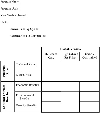
FIGURE 3-1 Results matrix for evaluating benefits and costs prospectively.
nitions for multiple scenarios and will facilitate comparisons across programs. To ensure consistency, it is important for the scenarios used in the review of different programs to be built on precisely the same assumptions (e.g., the same oil and gas price assumptions); it is not sufficient for them to be similar in some high-level or vague sense.
The committee used the three scenarios that are currently used by DOE’s Office of Fossil Energy (FE) in its own benefits analysis (NETL, 2004). The committee reviewed these scenarios and felt that they succinctly highlight key issues that have wide-ranging effects across all of the FE and Office of Energy Efficiency and Renewable Energy (EE) programs. Moreover, having already been used by DOE, these scenarios provide consistency and familiarity for future analyses. The three scenarios are as follows:
-
The Reference Case, developed by the Energy Information Administration and described in the Annual Energy Outlook (AEO) (EIA, 2004). The AEO provides detailed forecasts of U.S. energy supply, demand, and prices through 2025. This scenario represents the government’s official base-case forecast. The 2004 Reference Case assumes as follows:
-
World oil prices decrease from their current levels to about $24 in 2010 and then increase to about $27 per barrel in 2025.
-
Significant increases in natural gas consumption—i.e., 23 trillion cubic feet (Tcf) to 26 Tcf in 2010 and 31 Tcf in 2025—with prices decreasing from current levels to $3.49 per thousand cubic feet (Mcf) in 2010, then increasing to $4.47 per Mcf in 2025.2
-
An increase in primary energy consumption from 97.7 quadrillion British thermal units (quads) in 2002 to 136.5 quads in 2025.
-
GDP growth of 3.0 percent per year to 2025.
-
Carbon dioxide emissions from energy consumption growing from 5,729 million metric tons in 2002 to 8,142 million metric tons in 2025.
-
-
The High Oil and Gas Prices scenario assumes that oil prices will remain very high throughout the period and that constraints on natural gas supply lead to higher natural gas prices and higher electricity prices. For example, the oil price in 2012 in this scenario is $33.41 versus $23.98 in the Reference Case, and the natural gas price in 2012 is $4.53 per Mcf versus $3.92 per Mcf in the Reference Case.
-
The Carbon Constrained scenario, developed by the DOE, assumes that U.S. emissions of carbon are constrained in response to environmental concerns. Specifically, this scenario assumes that the Global Climate Change Initiative goal of an 18 percent reduction in national greenhouse gas intensity (below the 2002 level) is achieved by 2012 (White House, 2002) and that annual emissions are held constant at
-
that level thereafter. Relative to the Reference Case, this leads to increased demand for natural gas and increased prices (for example, $6.79 per Mcf in 2012 versus $5.54 per Mcf in 2012 in the 2004 Reference Case) as well as greater reliance on renewable electricity, unless carbon sequestration technologies are successful.
Each of these scenarios represents an alternative future for a very complex energy system. For this reason, an equilibrium model like the National Energy Modeling System (NEMS)—as used by EIA and DOE—is useful for understanding the many implications for the highly interdependent energy system and economy. The committee recommends using NEMS (or an equivalent model) to establish the price and quantity parameters consistent with each scenario as the fundamental basis for benefits calculation. The market allocation (MARKAL) model could be used to extend these scenarios beyond the 25-year horizon currently considered by NEMS. The Reference Case is described in great detail in the Annual Energy Outlook, and the other scenarios are described in more detail in NETL (2004).
The committee reviewed DOE’s EE and FE programs to see how they relate to these scenarios. In the committee’s estimation, approximately 35 percent of the FE programs contributed value primarily in the Carbon Constrained scenario and 10 percent contributed value primarily in the High Oil and Gas Prices scenario; the remainder (55 percent) contributed value in the Reference Case as well as in the other two scenarios. In the committee’s estimation, approximately 15 percent of the EE programs contributed value primarily in the Carbon Constrained scenario and 40 percent contributed value primarily in the High Oil and Gas Prices scenario; the remainder (45 percent) contributed value in the Reference Case, as well as these other two scenarios.3 This review of the programs gave the committee confidence that these three scenarios take into account key issues across the programs and that they would be helpful in evaluating the FE and EE programs.
The three scenarios considered in the prospective benefits matrix are not intended to capture everything that could happen in the future. Indeed, there are an uncountable number of different possible futures, including other levels of oil and gas prices and carbon constraints. Therefore, the committee does not encourage reviewers to specify probabilities for these scenarios or to calculate a single “expected benefit” that represents a probability-weighted average across the three scenarios. Rather, the three scenarios are intended as a representative set of scenarios that highlight particular policy issues and provide a form of sensitivity analysis for the benefits analysis. Displaying the results across the three scenarios rather than collapsing the scenarios into a single expected value allows reviewers to focus on scenarios that they view as more likely or as representing particular policy objectives or interests. For example, a policy maker contemplating constraints on carbon emissions might look carefully at benefits in the Carbon Constrained scenario to see what DOE is doing to help prepare the United States for this possibility.
Projects and programs may yield benefits in some but not all scenarios. For example, the carbon sequestration program was viewed by the expert panel as providing benefits only in the Carbon Constrained scenario. In the two other scenarios, the panel did not believe the sequestration technology would be deployed and it would thus yield zero benefit. But even if the benefit of a program is zero for a given scenario, it is important that all program evaluations consider benefits in all of the scenarios. While carbon constraints or high oil and gas prices might not be particularly relevant to the performance of lighting technologies, the economic benefit associated with efficiency enhancement might vary across scenarios as electricity prices change.4 Even if the benefit does not change, the scenarios should be considered and expected benefits reported, because at some point reviewers may combine benefits across projects or programs for a particular scenario, and the absence of an estimate for benefit in a given scenario should not be confused with zero benefit.
While these three global scenarios should serve to illustrate the potential benefits of most DOE applied R&D programs, if a particular program is designed to provide benefits under some other set of circumstances, the DOE and/or review panels are invited to consider benefits in additional scenarios. In such a case, the alternative scenario should be described clearly and its benefits for this scenario should be calculated and reported in a manner consistent with the principles outlined elsewhere in this report. It should be considered in addition to the three global scenarios considered in the prospective benefits matrix—that is, it should not be viewed as a substitute for or a modification of one or more of those scenarios.
While the three scenarios considered here provide a good starting point for future panel evaluations, the committee recognizes that the scenarios or specific details may need to change to remain relevant to the prevailing policy environment. The committee recommends that the oversight panel (described in Chapter 4) consider revisions to scenarios annually, and that policy makers must have input in their selection and modification. An outcome of the process might be, for example, routine updates of the Reference Case scenario consistent with the most recent Annual Energy Outlook.
However, there is a trade-off here: Frequent (e.g., annual) updates help keep the scenarios relevant but make it difficult to compare analyses performed in different years under different assumptions. Further, one might consider incorporating additional scenarios that highlight new policy issues as they arise. However, considering too many scenarios will increase the burden on those performing the analyses as well as those reviewing them. The key is for the analyses to consider the correct small set of scenarios and use them consistently.
GUIDELINES FOR CALCULATING BENEFITS
The retrospective study (NRC, 2001) defines benefits and provides rules for their calculation in its Appendix D. Economic net benefits are based on changes in the total market value of goods and services that can be produced in the U.S. economy under normal conditions, where “normal” refers to conditions absent energy disruptions or other energy shocks. Economic value can be increased either because a new technology reduces the cost of producing a given output or because the technology allows additional valuable outputs to be produced by the economy. Economic benefits are characterized by changes in the valuations based on market prices. This estimation must be computed on the basis of comparison with the next-best alternative, not some standard or average value.
Environmental net benefits are based on changes in the quality of the environment that have occurred, will occur, or may occur as a result of the technology. These changes could occur because the technology directly reduces the adverse impact on the environment of providing a given amount of energy service, for example by reducing the sulfur dioxide emissions per kilowatt-hour of electric energy generated by a fossil-fuel-fired power plant, or because the technology indirectly enables the achievement of enhanced environmental standards, for example by introducing the choice of a high-efficiency refrigerator. Environmental net benefits are typically not directly measurable by market prices. They can often be quantified in terms of reductions in net emissions or other physical impacts. In some cases market values can be assigned to the impacts based upon emissions trading or other indicators.
Security net benefits are based on changes in the probability or severity of abnormal energy-related events that would adversely impact the overall economy, public health and safety, or the environment. Historically, these benefits arose in terms of “national security” issues, initially the assurance of energy resources required for a military operation or a war effort. Subsequently they focused on dependence upon imported oil and the vulnerability to interdiction of supply or cartel pricing as a political weapon. More recently, the economic disruptions of rapid international price fluctuations from any cause have been emphasized.
These three classes of benefits have been chosen to reflect the programmatic goals of the three DOE offices for which the study was conducted. They are not meant to be comprehensive. For example, they do not include the benefits of fundamental research sponsored by the Office of Science, health benefits, or other quality of life benefits that could be unintended but real consequences of some applied R&D programs. In order to use a similar methodology for other government agencies, it would be necessary to identify the fundamental classes of benefits associated with the programmatic goals of those other agencies rather than simply to use the three classes of benefits identified here.
Based on the experience of the expert panels convened for this project, the committee concludes that the fundamental definitions and guidelines developed for the retrospective study remain suitable for prospective benefits evaluation. These definitions and guidelines are consistent both with economic literature devoted to methods for estimating economic net benefits and with a smaller, but still substantial, literature on methods for estimating environmental net benefits. As pointed out in Energy Research at DOE: Was It Worth It? (NRC, 2001, p. 87), “security net benefits are a special class of economic net benefits or environmental net benefits, differentiated from those categories of benefits by their low likelihood or their infrequency of occurrence.” Thus, while there has not been much literature on estimating security net benefits, the literature on economic net benefits and environmental net benefits can be applied to this class of benefits.5
However, some additional guidelines are required to ensure that several issues important in prospective analysis are treated consistently:
-
Discounting net benefits to be received in future years.
-
Calculating the expected values of benefits.
Discounting Net Benefits
Typically, R&D involves expenditures in current and near-term-future years in order to receive gains, or benefits, in more distant future years. But a dollar’s worth of goods and services received (or spent) in distant years is worth less in the economy than a dollar’s worth of goods and services received (or spent) now, even when goods and services are measured in terms of “real dollars,” dollars adjusted to remove the effects of general price inflation. The economic discount rate provides a measure of the trade-off between goods and services received at different times. And because the net economic benefit is based directly on the market value of goods and services, the economic discount rate provides a
|
5 |
However, more work is required on the definition of security benefits. The committee deferred this issue to Phase Two. See Chapter 6 for a further discussion of Phase Two. |
TABLE 3-1 Effect of Applying a 3 Percent Discount Rate to a Lump Sum Cash Payment
|
|
Received in 10 Years |
Received in 30 Years |
Received in 50 Years |
|
Real benefits in the future ($) |
100,000 |
100,000 |
100,000 |
|
Discount factor formula |
[1/(1.03)]10 |
[1/(1.03)]30 |
[1/(1.03)]50 |
|
Value |
0.74 |
0.41 |
0.23 |
|
Present value of benefits ($) |
74,000 |
41,000 |
23,000 |
measure of the trade-off between net economic benefits received at different times.6
If a benefit will be received at a future time, t years from now, then under generally accepted discounting procedures, this future benefit is discounted to the current time by multiplying the benefit by the discount factor [1/(1 + r)]t, where r is the discount rate and t is the number of years in the future. The discount rate r is specified by OMB for government decision making. Currently OMB recommends a real discount rate of approximately 3 percent per year for cost-benefit analysis with long time horizons (OMB, 2004, Appendix C). The committee endorses this recommendation.
For example, using the 3 percent real discount rate, $100,000 of benefits received 10, 30, or 50 years in the future would be discounted by the factors shown in Table 3-1. This discounted value is generally referred to as the present value of benefits.
Calculating the Expected Value of Benefits
Calculation of net benefits typically starts with estimating the benefits conditional on a particular outcome under a particular global scenario. For example, benefits could be conditional on the R&D effort achieving technical success and resulting in products that will be adopted by consumers, business, or government. Generally a program manager cannot be sure that such an outcome will occur. The estimate of benefits would typically be different for other outcomes. As discussed below in the subsection “Decision Tree,” the committee’s recommended methodology involves assessment of the probabilities of the various possible outcomes. Therefore, the value reported for the benefits of an applied R&D program should be a single quantity that incorporates information about the various possible outcomes and their respective probabilities and levels of benefits. Including all
TABLE 3-2 Expected Benefits Calculation Given Three Possible Outcomes
|
|
Very Successful |
Moderately Successful |
Failure |
|
Conditional benefits ($) |
100,000 |
30,000 |
0 |
|
Probability |
.1 |
.5 |
.4 |
|
Product ($) |
10,000 |
15,000 |
0 |
such information is particularly important when the probability of meeting a program’s stated goal is low, since significant benefits may accrue from performance levels below the target level.
Accordingly, the committee recommends that the expected value of net benefits (or, for short, “expected benefits”) should be calculated as the probability-weighted average of benefits for all important outcomes analyzed under a particular global scenario. To illustrate, assume that a project could have three different levels of success (i.e., outcomes)—very successful, moderately successful, and failure—each having a different conditional benefit measured in dollars. An overall analysis would assess the net benefits to the United States for each of these possible outcomes and would assess the probability of each outcome. Then the conditional benefit of each outcome would be multiplied by its probability and the three products would be added together to give the expected value of benefits.7 (Note that the probabilities of all the outcomes must total to 1.0.) This is illustrated in Table 3-2, using assumed values of the three conditional benefits and assumed probabilities. The expected benefit of the project illustrated in Table 3-2 is the sum of the three products—$10,000, $15,000, and $0—or $25,000.
Note from the example that both the moderately successful and the very successful outcomes contribute to the expected benefit. If the analysis had considered only the most successful outcome, there would be only a $10,000 expected benefit. If the analysis had considered only the most likely outcome, there would be only a $15,000 expected benefit. Only by including all of the possible outcomes would the analysis correctly determine the expected benefit of the project.
Although in principle the analysis should include all possible outcomes, in practice very unlikely outcomes can be ignored unless they provide extraordinary benefits. For example, assume that in the example in Table 3-2 there was another possible outcome even more successful (“spectacu-
TABLE 3-3 Expected Benefits Calculation Given Four Possible Outcomes
|
|
Spectacularly Successful |
Very Successful |
Moderately Successful |
Failure |
|
Conditional benefits ($) |
150,000 |
100,000 |
30,000 |
0 |
|
Probability |
.01 |
.09 |
.5 |
.4 |
|
Product ($) |
1,500 |
9,000 |
15,000 |
0 |
larly” successful) than the very successful outcome but that it was very unlikely, having, say, a probability of .01. Assume further that the spectacular outcome would result in a benefit of $150,000. Inclusion of that spectacular though unlikely outcome would give the results shown in Table 3-3.
The expected benefit of the project depicted in Table 3-3 is the sum of the four products—$1,500, $9,000, $15,000, and $0—or $25,500. Although this expected value is larger than the $25,000 figure calculated in Table 3-2, the difference is insignificant, given that all of the numbers are only approximations. Similarly, combining the spectacularly successful outcome with the very successful outcome, assessing the conditional benefit of the combined outcome as equal to that of the very successful conditional benefits ($100,000), and assessing the probability as equal to the sum of the two individual outcomes, or .10, would have led to an expected benefit only slightly different than that shown in Table 3-3.
The situation would be different, however, if the benefits of the most successful project were extraordinarily (rather than just “spectacularly” high). For example, assume that the benefit of the most successful project is $2,000,000, not $150,000. In that case, the calculation would be shown in Table 3-4. The expected benefit of the project is the sum of the four products—$20,000, $9,000, $15,000, and $0—for a total of $44,000. This expected benefit value is sufficiently larger than the $25,000 calculated in Table 3-2 that explicit consideration of the very low probability/high conditional benefits outcome would be important. The impact of an outcome on the expected benefits is a useful test of which out
TABLE 3-4 Expected Benefits Calculation Given Four Possible Outcomes, One of Them “Extraordinary”
|
|
Extraordinarily Successful |
Very Successful |
Moderately Successful |
Failure |
|
Conditional benefits ($) |
2,000,000 |
100,000 |
30,000 |
0 |
|
Probability |
.01 |
.09 |
.5 |
.4 |
|
Product ($) |
20,000 |
9,000 |
15,000 |
0 |
comes are important enough to consider in the decision tree analysis, which is discussed next.
THE DECISION TREE FRAMEWORK
Introduction
As is discussed in the section above, the estimated benefit of a program is subject to multiple sources of uncertainty, both in what happens in the program itself and what happens to the alternative technologies or the policy environment. The basic principle of program assessment remains the same as in a retrospective analysis: Find the difference between social benefits with the government program and without it. However, the implications of the various uncertainties must be considered carefully. In this section, the formal mechanism developed by the committee for estimating benefits—the decision tree framework—is described. First, some of the key factors to consider in benefit assessment are discussed.
Key Factors in Benefit Assessment
Both the retrospective study and subsequent work done by DOE developed useful methodologies for the computation of benefits. In some cases, the computational method can be very complex. (The next section of this chapter, “Simplified Model for Estimating Benefits,” outlines a simplified computational method that nevertheless relies on a general equilibrium model like NEMS to create internally consistent price and quantity schedules.) Whatever the complexity of the computational method, it is essential first to define the outcomes for which it is worth calculating the benefits. Three factors typically determine the alternative outcomes of an applied R&D program. One (or two) of the factors might not be important in a specific case, but their ubiquity implies that each assessment should look at all three so that analysis teams can determine which of them need to be explicitly incorporated into the benefit calculations. Each is discussed briefly.
Estimating the Net Benefit of Government Support
An estimation of the expected net benefit of a government program involves an explicit or implicit comparison of the possible outcomes present with the government program and the possible outcomes absent the program. For example, a government program might lead to a research team making a significant technology advance. The expected benefits of that advance could be estimated. However, to determine the net benefits of the government support, it is necessary to consider the extent to which this or other research teams are likely to have achieved the same technology advance absent the government support and to estimate the benefit and probability of the advance. The expected net benefit of the gov-
TABLE 3-5 Effect of Next-Best Technology on Expected Benefits
|
|
Very Successful Government Program |
Moderately Successful Government Program |
||
|
Substantial Improvement in Next-Best Technology |
No Improvement in Next-Best Technology |
Substantial Improvement in Next-Best Technology |
No Improvement in Next-Best Technology |
|
|
Conditional benefits of government technology program ($) |
50,000 |
112,500 |
0 |
37,500 |
|
Probability of next-best technology’s success |
.20 |
.80 |
.20 |
.80 |
|
Product ($) |
10,000 |
90,000 |
0 |
30,000 |
|
Expected benefits of government program ($) |
10,000 + 90,000 = 100,000 |
0 + 30,000 = 30,000 |
||
ernment program is the difference between the expected benefits with and without government support, not the expected benefit of the technology advance with government support.8
Considering the Uncertainty Surrounding the Next-Best Technology
Similarly, estimation of the expected net benefits of a government program requires either explicit or implicit consideration of how the market would evolve without the technology being developed by the DOE research program. Take, for example, the estimation of net benefits of a successful government program for new solid state lighting technology. One could assess the benefits of the new lighting technology advance assuming it is coupled with a government program designed to hasten its market adoption. One would have to compare these benefits with those of a program designed to hasten the adoption of the next-best lighting technology—say, the next generation of compact fluorescent lights. It would not be appropriate to estimate the expected net benefits based on a comparison with the existing generation of compact fluorescents or (and this would be even less appropriate) the existing generation of incandescent lighting technology.
In some cases, there might be considerable uncertainty about the benefits that accrue due to advances in alternative technologies; in some cases the benefits might change radically depending on potential, but uncertain, advances in the next-best technology. Commercial penetration of a moderately successful fuel cell car, for example, might be substantially reduced if the fuel efficiency of hybrid-electric vehicles improves dramatically. In cases such as this, it may be necessary to consider explicitly different levels of success for the next-best technologies and the probabilities that these levels will occur.
Consider again the example in Table 3-4. Assume that when the program outcome is “extraordinarily successful” it dominates the market for any plausible advances in the next-best technology. The markets for the less successful cases—that is, “very successful” and “moderately successful”—will decline as the next-best technology improves. Suppose the next-best technology has an 80 percent chance of remaining the same as today but a 20 percent chance of a substantial improvement; this would reduce the market for the “very successful” and “moderately successful” outcomes by the amounts shown in Table 3-5.
Considering Enabling/Complementary Technologies
In many cases, estimating the expected net benefits of a government program requires either explicit or implicit consideration of enabling or complementary technologies. Whenever the market acceptance of a particular technology depends strongly on the existence of other technologies complementing the technology in question or enabling it, it is necessary to assess the probability that enabling or complementary technology will be successful. For example, a successful government program to advance the technology of hydrogen fueling stations for light-duty vehicles would have little benefit unless the various technologies for hydrogen vehicles—particularly fuel cells and onboard storage—were to advance enough that many people would choose to purchase hydrogen fuel cell vehicles; thus it is necessary to assess the probabilities that these complementary technologies will be successful in order to accurately estimate the net benefits of the government program to advance the technology of hydrogen fueling stations.9
In some cases, the benefits of a program are greatly enhanced by complementary technologies but the program will provide at least some value even in their absence. If the distinction is important, then an assessment of the probability of success for the complementary technology and the expected benefits of the program considering both potential outcomes—the benefits of the program with and without the complementary technology—will be needed. This involves a calculation equivalent to that shown in Table 3-5.
Decision Tree
The committee recommends the application of a decision tree process that requires consideration of the three key components of government energy R&D program evaluation and clarifies the relationships among them. Figure 3-2 illustrates
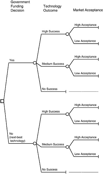
FIGURE 3-2 Decision tree.
the possible relationships among these three key components using a decision tree, where the first node (the decision node) represents the government action—to pursue the program or not; the second node (first chance node) is the possible outcome of the program; and the third node (second chance node) represents the multiple factors that determine market acceptance, including developments in the next-best technology and the success of enabling and complementary technology programs.
The tree illustrates the many different possible combinations of outcomes of the research program. The topmost path, for example, represents the case where (1) government funds the program, (2) the program has a high level of success, and (3) the technology achieves a high level of market acceptance. Other paths illustrate the case where the program is funded and successful but market acceptance is nevertheless weak or absent; where the program itself is not as successful but the technology is nevertheless accepted in the market, and so on. The lower part of the figure represents cases where the government program is not funded. The technology—or an alternative technology deemed the next best—may be successful or moderately successful, depending on private R&D efforts, and market acceptance again can make that investment and technological outcome commercially successful or not.
The decision tree provides a framework for organizing the benefits calculation. As discussed in the next section, a simple benefits calculation model would be used to calculate benefits in each scenario represented by a path through the tree. The expert panel must specify probabilities for the various uncertainties in the tree. Because the probabilities need not be the same in each global scenario, the expected benefit could differ in each scenario. (See discussion above in the section “Scenarios.”) Then, as discussed in the preceding section, the value of the government program is the difference between the expected benefit of the with-government-support alternative and that of the without-government-support alternative.
In principle, each potential outcome must be considered when evaluating government programs. In practice, however, evaluators need only accommodate those features that are important in a specific case. As discussed in Chapter 4, the committee believes that an expert panel can identify the significant outcomes. An example of the development of a full decision tree and its reduction to a few significant outcomes is shown in the report of the expert panel on the carbon sequestration program in Appendix G.
Figure 3-3 illustrates the decision tree applied to the advanced lighting program, with numerical values included. These numerical values are not to be taken as the committee’s estimates of the benefits but are provided only to show the general structure of such a decision tree and to illustrate the calculations that would be used. The committee’s estimates of the benefits of lighting R&D can be found in Chapter 5 in the section “The Lighting Panel.”
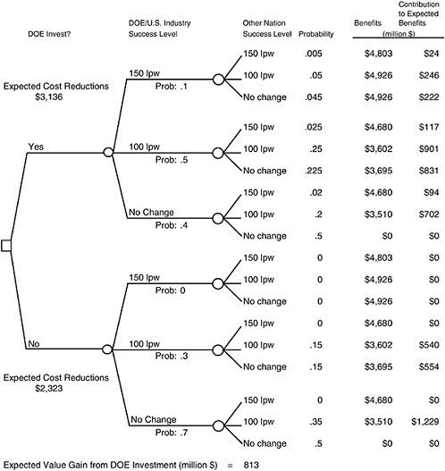
FIGURE 3-3 Example of decision tree applied to advanced lighting programs (for illustrative purposes only).
In this decision tree, the government has one basic decision, to invest in the R&D program or not to invest. In either case, three possible levels of lighting efficacy could be achieved by U.S. industry: 150 lumens per watt (lpw), 100 lpw, or no change from the current situation. If DOE invests, then the probability of the greatest advance, 150 lpw, would be increased to 10 percent (from 0 percent in the absence of DOE research); the probability of the medium advance, 100 lpw, would be increased to 50 percent (from 30 percent in the absence of DOE research); and the probability that there would be no advance would be decreased to 40 percent (from 70 percent in the absence of DOE research). Note that these probability assessments do not show that DOE investment will guarantee success—they show that DOE investment increases the probability of successful outcomes.
DOE investment also can change the probability that other nations will have R&D successes. This decision tree assumes that there will be a 5 percent probability that other nations will achieve 150 lpw if DOE conducts a research project but no probability of that success in the absence of DOE research. It assumes that there will be a 50 percent probability of other nations achieving 100 lumens per watt, with or without DOE investment.10 With DOE research, there is a 45
percent probability that other nations will not have any incremental improvement; without DOE research, that probability would be 50 percent.
Given those probabilities of U.S. and foreign success, the probabilities of the combinations of outcomes are given in the left column. For example, the probability of U.S. industry achieving 150 lpw and other nations achieving 100 lpw is .05, calculated as the product of .10 and .50.
The second column provides sample benefit estimates for the combinations of outcomes. Here again, the numbers are presented only for the purpose of illustration. For example, the benefit to the United States of U.S. industry achieving 150 lpw and other nations achieving 100 lpw is $4,926 million.
The contributions to the expected value are given in the third column, as the product of the numbers in the first and second columns. The contribution to expected value of the combination—U.S. industry achieving 150 lpw and other nations achieving 100 lpw—is $246 million, the product of .05 and $4,926 million.
The expected value of all possible combinations of outcomes, given DOE R&D investment, is the sum of the top nine numbers in the column on the right. This sum is $3,136 million. The expected value of all possible combinations of outcomes if DOE makes no such R&D investment is the sum of the bottom nine numbers in the column on the right. This sum is $2,323 million.
Note that as a result of U.S. industry R&D and R&D in other nations, the United States would capture benefits even without DOE investment. But those benefits would be smaller than they would be if DOE did invest in R&D.
The difference between the benefits with DOE investment—$3,136 million—and the benefits absent DOE investment—$2,323 million—is the expected value of the gain resulting from DOE investment. This difference of $813 million is the overall benefit from the DOE investment. The overall benefit is not the benefit with DOE investment—$3,136 million—since a large share of those gains to the United States would occur even without DOE investment.
Expert Evaluation of Probabilities
Evaluating the probabilities associated with the different branches on the tree—the likelihood of technical success for the program and the likelihood it will achieve different levels of market penetration—is a critical part of the work of the expert panels. The committee believes that independent panels of experts can provide appropriate estimates using the process described in the section “Panel Activities and Process,” in Chapter 4. To guide the expert panels, the committee developed the guidelines in the following subsections for assessing probabilities at each of the nodes in the decision tree.
Government Program Support (Decision Node)
The difference between paths with and without the government program is a measure of the government role. As indicated earlier, evaluation seeks not just to measure change that accompanies a government program, project, or other activity, but also to determine whether the change is attributable to specific government intervention. Evaluation must rule out alternative, competing explanations for an observed or predicted change. For example, a government program may be launched to develop a new energy-conserving technology, and, indeed, it may succeed. But the same outcome, or a portion of it, may have resulted without the government program. The decision tree methodology suggests using a counterfactual approach in the attempt to isolate or demonstrate the effects of the program under evaluation. In a decision tree analysis, one branch describes the path if a specified government program with identified characteristics, including a defined level of funding, is adopted. An alternative branch of the tree describes the path without that government program. Other branches may describe the path of the government program at various funding levels. The probabilities and values for the paths along each branch are based on the assumption that the program is funded at the specified level. By comparing the resulting expected value benefits for alternative branches, the differential expected benefits attributable to the government program can be identified.
A government program may affect societal benefits in multiple ways, including the following:
-
The program may result in technology development and use that otherwise would not have occurred. If it is thought that nothing would have happened in the foreseeable future without the government program, this is captured in the benefits stream for the without-government-program branch. The only benefits associated with the without-government-program branch are those attributable to the next-best technology available when the government program would have been completed.
-
The program may accelerate technology development and use. If the government program is viewed as causing the development and use of a technology that otherwise would be developed in the same way but at a slower pace, this effect is captured in the timing of the estimated stream of benefits underlying the benefit calculations at the end of the with-government-program branch as compared with the timing of the benefits stream at the end of the without-government-program branch. For example, if the with-government-program branch is expected to result in the technology being developed and adopted into use, say, 3 years faster than the without-government-program branch, the stream of benefits will be shifted forward by 3 years and the government’s contribution will be credited with the difference in the expected present value of the two benefits streams.
-
The program may improve a technology and make it more attractive to users. If the government program provides significant advances over the next-best technology, this can be captured in several ways. The advance may increase the probability of market acceptance. It may improve market penetration. It may generate larger unit benefits in use. Each of these effects can be captured in one of the branches of the decision tree.
-
The program may increase the probability of technical or market success. If the government program reduces the risk associated with achieving technical or market success, this is captured in the comparative probabilities assigned to the with- and without-government-program branches of the tree in the technical and/or market risk decision nodes. If the government role is to reduce technical risk, a higher probability of technical success assigned to the with-government-program branch will result in greater expected benefits projection for that branch and a larger expected benefit will be attributed to the government program, calculated as the difference between the expected values of the with-and without-government-program branches.
-
The program may enlarge the scope of the technology to make it more “enabling.” Enabling technologies are characterized as generating larger-than-average spillover benefits; that is, benefits that accrue broadly in society rather than more narrowly to direct private-sector investors in the research. If the government program enlarges the scope of the technology in ways that create a more enabling technology platform, the effect is captured in the benefits stream of the with-government-program branch of the decision tree, which includes a larger societal benefit than the without-government-program branch.
-
The program may increase collaborative and multidisciplinary research. The government program may promote collaboration among researchers by helping to overcome existing barriers to collaboration. Networks of collaborative R&D activity are increasingly seen as playing an important role in innovation. If the government program increases collaboration and if increased collaboration increases the likelihood of technical or market success, this effect is captured by assigning different probabilities of success to the with- and without-government-program branches. If, on the other hand, the change in collaborative effort increases the scope of the research, increasing its enabling characteristics, this effect is captured in the with- and without-government-program branches as differences in the estimates of societal benefits.
-
The program may produce a combination of effects. If the government program is expected to have more than one of the effects listed above, these may affect both the comparative probabilities assigned to technical and market success and the comparative projected benefit streams estimated for the with- and without-government-program branches of the decision tree. Multiple effects can easily be accommodated in the context of the decision tree analysis. As in the other cases, it remains necessary to take the difference between the with- and without-government-program branches to find the expected benefits of the government program.
Technical Outcomes (First Chance Node)
In retrospective evaluations, one knows if a specific research program was successful in terms of meeting its technical (and commercial) objectives. In prospective evaluations, it is not known in advance whether a program will be successful. To calculate benefits one must therefore consider the likelihood that the program will be successful. While technical success can be viewed in relation to achievement of a single goal or outcome, a given research program might be judged successful across a range of outcomes, each with its own probability of technical success. As is discussed above, if the possibility of multiple outcomes is ignored, research benefits may be underestimated. Moreover, the use of a single “representative” outcome will usually be inaccurate and will mask assumptions about the relationships between the program outcomes and the alternative technologies.
DOE often identifies single goals for programs, and these goals may be stretch goals in the sense of being at the high end of possible outcome value but having a relatively low probability of technical success. Attaining less optimistic goals with delayed or only partial benefits may still have considerable value as well as a higher probability of technical success. Consideration of stretch goals alone is therefore also likely to lead to an underestimate of benefits. The number and nature of the outcomes to include will vary by project.
Probabilities of technical success (at any outcome level) are likely to depend on the level (and, in some cases, the quality) of resources—financial, technical, and managerial—expected over the life of the program, so that probabilities change with funding/resource level and the calculated expected net benefits are conditional on that level.
Market Risk (Second Chance Node)
“Market risk” refers to the probability of a given technology being moved out of the lab and deployed into use.11 This risk is expressed as a probability for each case under evaluation and entered into a third node for each relevant branch of the decision tree. It is critical to the estimation of expected
benefits, as an applied R&D program yields benefits only if the technology is used.
Probabilities are applied to market penetration estimates. The probability that a technology will be deployed is distinct from the rate at which it is deployed—that is, its market penetration. It is necessary to estimate the rate at which the technology will come into use.
Many factors influence whether, and to which extent, a technology will be deployed into use. These factors do not apply to all programs, and the committee recommends that the chief factors that influenced the probability estimates be identified in either a row at the top of the results matrix (see Figure 3-1) or in an appendix. These factors include the following:
-
Market demand. To what extent does the technology meet a current demand? Does it enable users to solve an important problem or exploit a promising opportunity?
-
Competition. What are the competing technologies that the target technology must overcome in order to be accepted in the market? Note that there are always competing technologies. Are others working on the same technology? Are others working on different technologies that might meet the same need? In the United States? Outside the United States? Who is performing the work?
-
Window of opportunity. How long will the need for the technology exist? Are there factors that might eliminate or reduce the need for this technology? For example, are advances in a competing technology likely to outstrip those in the target technology, wiping out its advantages? When might this occur?
-
Potential hazards. Are there potential environmental or safety concerns that might limit the use of the technology? For example, are there any by-products that might create an environmental or biological hazard, incurring mitigation costs or exposure to liability?
-
Ease and cost of implementation. To what extent does adoption of the technology require changing existing systems or ways of doing things? For example, it would be easy to introduce a new catalyst into an existing reactor. On the other hand, a hydrogen-powered automobile would require a new fuel distribution system if the hydrogen is centrally produced, making implementation more difficult. To what extent will adoption of the technology require large capital investment? To what extent will adoption cause disruptions and downtime in current operations? To what extent will adoption require worker retraining?
-
Resistance by special interests. To what extent will those adversely affected by the new technology lobby to retard its adoption, and how successful are they likely to be?
-
New regulations. To what extent are new regulations likely to promote or impede the adoption of the technology? For example, unexpectedly stringent environmental regulations on diesel emissions made obsolete the fuel and engine research programs designed to meet the more modest objectives that had been anticipated. Conversely, adoption of appliance efficiency standards can lead to development of new technologies, as in the case of refrigerators (NRC, 2001, pp. 97-98).
-
Complementary and prerequisite technologies. Is adoption of the new technology dependent on the availability of other technologies? Are these technologies still in the pipelines of other R&D programs? Will they be available in time to support the technology under evaluation?
Market risk factors are often critical to evaluating the potential of an R&D program. Indeed, for investments in fairly specific technologies, the risks associated with market acceptance may overwhelm those associated with technical success. Alternatively, fundamental programs that yield results applicable to a range of technologies and market conditions may be less susceptible to the market risks discussed here: They may be applicable in a wide range of regulatory regimes and may contribute to multiple technologies, at least some of which are likely to be available and of interest in the relevant time frame. Of course, long-term fundamental programs may be very risky in that the likelihood that all of their goals are achieved is remote.
Long-term, fundamental R&D requires further development and often further research before reaching a commercial outcome. Applied R&D such as the DOE programs considered in this report aims to develop technologies with specific performance and cost criteria that will be commercial in a time frame consistent with the schedule of the applied R&D project. It is this latter type of R&D having more immediate commercial applicability that the methodology has been designed to evaluate. The types of benefits evaluated in the methodology—for example, economic benefits—are consistent with the goals of technology development programs and the expectations of those making the investments. A further difference between fundamental and applied R&D is that the former has knowledge as its primary goal while the latter has knowledge as a by-product. Because the methodology proposed here is for applied R&D, it has economic, environmental, and security benefits as its primary goal and does not give credit for knowledge generated in the course of a technology’s development.
Recommended Approach for Assessing and Using Probabilities
Chapter 4 provides a detailed description of the process the committee recommends for evaluating an R&D program, including assessing the probabilities. As part of this process, the committee suggests that after an initial meeting to frame the evaluation, each panel member should specify probabilities for the key uncertainties in the program by completing a questionnaire. This will give each panel member an opportunity to reflect his or her own beliefs concerning the uncertainty. If a committee member is not comfortable specifying
a probability for some event, he or she need not do so. For example, an economist on the panel may decline to assign probabilities related to technical aspects of a particular program. However, the composition of the committee should be such that, for each of the critical uncertainties in the problem, there are several expert panelists who have substantive knowledge.
At the second meeting, the panelists would review their individual probability assessments and discuss the rationale for them. In this way, differences in assumptions and beliefs of the panelists will surface and can be debated. After this discussion, the committee members would be given the opportunity to revise their individual assessments in light of what they learned in the discussion.
While the discussion will help ensure that the panelists share the same assumptions, it will not cause them to agree on probabilities. Indeed, given the difficult questions likely to be encountered in these evaluations, disagreement about probabilities should not be surprising. Rather than trying to reach a consensus, the committee encourages considering and reporting the full range of expert probabilities and the implied range in expected benefits. For example, in the sequestration study, the summary report in Appendix G describes the full range of probabilities and expected benefits (see Figures G-5 and G-6). However, to keep the summaries’ descriptions simple, the committee suggests reporting the average expected benefit—that is, the average of the expected benefits of the different expert panelists. The literature on forecasting and probability assessment has consistently shown that the errors associated with these average estimates tend to be less than the average error in the individual estimates. Including the range of probabilities and expected benefits in the evaluations in the discussion will, however, give the reader a sense of the range of disagreement associated with these quantities.
SIMPLIFIED MODEL FOR ESTIMATING BENEFITS
The calculation of the expected benefits of an R&D program using the decision tree approach must consider the calculation of benefits in many specific outcomes, each represented by a path through the tree. To avoid making the benefits evaluation process excessively burdensome, the committee recommends the use of simple computational models wherever possible. These models may be simple spreadsheet models or back-of-the-envelope calculations. They must be easy to work with, and their assumptions and calculations should be reasonably transparent to reviewers.
DOE has been using NEMS to calculate benefits, and the expert panels all considered the use of NEMS for this purpose. However, their experience identified three problems. One is the lack of transparency—the difficulty of identifying the critical assumptions on which the NEMS calculation is based. Second, it appears that NEMS does not calculate net benefits using the rules established in Appendix D of the retrospective report (NRC, 2001) and recommended by the committee for prospective calculations as well.12 Finally, running NEMS is both cumbersome and very resource intensive, which greatly limit its utility for exploring alternative scenarios and program outcomes. All of the panels encountered these difficulties, underlining the need for a different procedure for calculating benefits.
The following discussion lays out a very simple procedure for estimating net benefits, a procedure useful for a wide range of projects. This procedure will require estimates of prices and quantities of the various energy commodities in a scenario-specific market equilibrium, for the relevant time horizon, at a level of detail consistent with the new technology being examined. Typically, such data could be derived from a large-scale energy model. The committee believes that NEMS is, in fact, suitable for this purpose. For this discussion, it is assumed that a scenario-specific NEMS market equilibrium will be used to provide the data, although other models could presumably be chosen, e.g., reduced-form versions that approximate the more detailed modules in translating input variables (e.g., prices for demand or quantities for supply) to output variables (e.g., quantities and investments for demand and prices and investment for supply). Reduced-form versions can be easily substituted for the full modules. They would not be independent models but would be simple mathematical structures estimated from the original modules to approximate these modules’ full responses (NRC, 1992).
Two classes of technology changes will be considered here. The first class, generically referred to as “energy efficiency advances,” aims to increase the efficiency with which energy services are delivered to individuals or firms but not to change the nature of energy services used by the consumer. Examples would include advances in lighting technology that allow the same quality of light to be obtained using less electricity per lumen or advances in the energy efficiency of refrigeration or of heating, ventilating, and air-conditioning (HVAC) systems. Increases in the conversion efficiency of electric generators or reductions in the capital cost of oil refineries could also fall into this category. The essential characteristics are that (1) the average cost of providing a good or service is reduced as a direct result of efficiency gains or reductions in the inputs needed to produce the good or service and (2) the quantity of the good or service used may change, but not by a very large percentage.13
The second technology, generically referred to as a “resource supply enhancement,” aims to increase the amount of a good or service that can be produced for a given unit cost, provided that the market value of that good or service exceeds the additional cost of its production. Examples would include advances in natural resource exploration that would
allow new resource deposits to be discovered at costs significantly lower than the value of the deposits or additional quantities of oil and gas to be produced.14 The essential characteristics of this category are that (1) the energy supply is increased as a direct result of reduced cost of production arising from the deployment of the technology being evaluated and (2) the equilibrium price of the resource involved may change, but not by a very large percentage.
The committee believes that most of DOE’s applied R&D programs are covered by these two possibilities. In particular, the simplified model could be applied in each of the programs that were evaluated for this project.
Analysis of Energy Efficiency Advances
In the first class of technology advance—energy efficiency advances—the primary component of benefits can be estimated in a straightforward manner by calculating the reduction in the quantity of inputs required to produce the same energy service and valuing those reduced inputs at their marginal cost. This reduction in the quantity of inputs multiplied by their marginal cost gives a good measure of the total value of inputs that would no longer be required to produce the fixed quantity of the energy service, say, the lighting service. These inputs would become available to produce other goods and services. In a competitive market, the total value of these no-longer-needed inputs would equal the total value of additional goods and services that they could be used to produce. Thus the reduction in the quantity of inputs multiplied by the marginal cost of those inputs gives a good measure of the changes in the total market value of goods and services that could be produced in the U.S. economy. As defined in Energy Research at DOE: Was It Worth It? (NRC, 2001), this change in the total market value of goods and services is the economic benefit.
For example, advances in lighting would lead to the use of less electricity to provide the same amount of light. The reduction in electricity use implies that less electricity would be generated, transmitted, and distributed to provide the same amount of lighting services. The primary component of the net economic benefit is equal to the reduction in the quantity of electricity (and other inputs) used to produce exactly the same lighting services multiplied by the marginal cost of providing that electricity (and other inputs). The marginal cost of electricity is the sum of marginal generation, transmission, and distribution cost of making that electricity available to its user. Changes in other inputs to be included might be changes in the capital costs of lighting or changes in the labor costs of periodically changing light bulbs, light emitting diodes, or other equipment used to produce the lighting services.
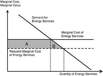
FIGURE 3-4 Benefits of energy efficiency advances. Energy price equals energy marginal cost.
The marginal cost of most goods and services corresponds closely to the competitive market price. In that case, the primary component of the net economic benefit is equal to reductions in inputs required to produce the same energy service multiplied by the price of those inputs, a case diagrammed in Figure 3-4. This figure represents the marginal cost of energy services for different amounts of energy services used. The marginal cost of energy services is the sum of all additional costs—capital, labor, and energy—required to produce one more unit of the energy service, for example, lighting. One component of this marginal cost is the additional energy required to produce the additional unit of energy services, multiplied by the price of that energy. This figure also represents the marginal value to the consumer or business of the additional energy service for different amounts of energy services used. This marginal value will typically be measured by the demand function for energy services. The crossing point of the two lines represents the optimal use of the energy services from the perspective of the energy user.
An energy efficiency advance that reduces the amount of energy needed to produce the same quantity of energy services would reduce the marginal cost of energy services.15 This is represented by the dashed line in Figure 3-4. The reduction in marginal cost is the difference in height of the dashed and solid lines.
The primary component of net benefits would be the area of the shaded rectangle in Figure 3-4, labeled A. In this figure, the reduction in marginal cost is the same for all levels of energy services and thus equal to the change in average cost.16 The area of rectangle A is simply the change in the average cost (of energy services) multiplied by the quantity. This area is equal to the change in the total cost of energy services provided.
A numerical example from the advanced lighting program will illustrate this calculation. Here again, the numerical assumptions are arbitrary. Assume that 50 million households each use 15 lightbulbs (100-watt bulbs) for 4 hours per day, 365 days per year. Each lightbulb provides 50 lpw, or 5,000 lumens. Thus the total energy services from these lightbulbs would be 5,475 trillion lumen-hours (50 million × 15 × 100 × 4 × 365 × 50). This would be the quantity of energy services per year in Figure 3-4. The marginal cost per lumen-hour for the United States would be calculated as the number of kilowatts per lumen multiplied by the marginal cost17 per kilowatt-hour, assumed to be $0.04. Thus the marginal cost per lumen-hour would be $0.0000008 ($0.04 per kilowatt-hour, divided by 50,000 lumens per kilowatt). The total cost of these energy services would be the product of $0.0000008 per lumen-hour and 5,475 trillion lumen-hours, or $4.38 billion.
If the R&D program achieved an efficacy of 100 lpw and all households replaced every lightbulb with the new, more efficient bulb, then the cost per lumen would be halved, becoming $0.0000004. The total cost of 5,475 trillion lumen-hours of energy services would be the product of $0.0000004 per lumen-hour and 5,475 trillion lumen-hours, or $2.19 billion. In this case, area A in Figure 3-4 would be the difference between $4.38 billion and $2.19 billion, or $2.19 billion per year.18
The shaded triangular area B would be calculated based on the increase in the amount of lighting that would be consumed if lighting became cheaper. Assume that every 10 percent decrease in cost per lumen would lead consumers to increase their lighting consumption by 2 percent (elasticity of demand equal to −0.2). Then, in response to the 50 percent decrease in the cost per lumen, electricity use would increase by 10 percent, or 547 trillion lumen-hours. Area B would then be equal to one-half the increase in lumen-hours multiplied by the reduction in cost per lumen-hour ($0.0000004 per lumen-hour), or $109 million. It should be noted that area B is only 5 percent of area A.
The calculations above assume that 100 percent of the lightbulbs would be replaced and that the new lightbulbs cost the same as the old bulbs. If the new lightbulbs were more costly, the total calculation would be adjusted by subtracting the additional cost of new bulbs. If only a fraction, say 20 percent, of the lightbulbs would be replaced by new ones, the benefits calculated above would be multiplied by that fraction. In this case, the total benefits would be $460 million per year.
In some cases, however, the marginal cost of an input does not correspond closely to the competitive market price of that input. For example, average cost pricing of retail electricity may lead to a significant divergence between the retail price and the marginal cost of providing that electricity. Such retail prices may include a large component for fixed costs, such as the capital and maintenance costs of wires, transformers, and other distribution assets. And surcharges included in electric rates to pay for historical costs—for example, historical costs of the Western electricity crisis—can increase retail prices to well above marginal costs. In that case, the retail price cannot be used to value electricity savings. Instead it would be necessary to directly estimate the marginal generation, transmission, and distribution cost of making that electricity available to its user. The quantity represented by area A would still be equal to the change in the total cost needed to provide the fixed quantity of energy services, but here the total cost change is the total cost of supplying the electricity, not simply the cost paid by the final consumer, a situation illustrated in Figure 3-5. In this figure
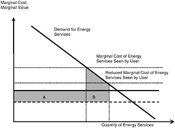
FIGURE 3-5 Benefits of energy efficiency advances. Retail price exceeds energy marginal cost, and the marginal cost to the user of the quantity of energy services is greater than the economy-wide marginal cost.
the dotted lines represent the original and reduced marginal cost of energy services as seen by the user—that is, the prices that the user pays. The lower solid and dashed lines are the actual costs of the energy service, as determined by the overall costs of making that service available to the user. The analysis is the same as that for Figure 3-4, except that the points at which the dotted lines and the demand curve cross represent the optimal use of the energy services from the perspective of the energy user.
A second potential component of the net economic benefit is based on changes in the use of the good or service whose cost has decreased. A reduction in the cost per unit of lighting services can be expected to lead people to use more lighting services. A similar response could be expected for many goods and services experiencing a per unit cost reduction.
Whether such a change in use becomes a quantitatively significant component of the net benefits depends on whether the marginal cost to the user of the additional goods or services is significantly different from the economy-wide marginal cost of producing and distributing those goods or services.
Figure 3-4 illustrates the calculation when the marginal cost to the user of the additional goods or services is the same as the economy-wide marginal cost of producing and distributing those goods or services. In this case there is an additional net benefit equal to the area of the triangle B. This area, if all the lines are straight, is equal to one-half of the change in marginal cost of energy services, multiplied by the change in the amount of energy services used. Typically this area is small relative to area A. Note that in Figure 3-4, the sum of areas A and B is equal to the change in the average cost of energy services multiplied by the average of (1) the original quantity of energy services before the energy efficiency advance and (2) the new quantity of energy services after the energy efficiency advance. In the lighting example, assuming that the only change is in the amount of electricity used per unit of lighting, the sum of these two areas would just equal the price of electricity multiplied by the average of the quantity of electricity used before the advance in energy efficiency and the quantity of electricity used after the advance in energy efficiency.
Figure 3-5 illustrates the calculation when the marginal cost to the user of the additional goods or services is greater than the economy-wide marginal cost of producing and distributing those goods or services. In this case there is an additional net benefit equal to the shaded area B. This area, if all the lines are straight, is equal to the change in the quantity of energy services used multiplied by the average of two differences: (1) the difference between the marginal cost of energy services as seen by the consumer and the actual marginal cost of energy services to the system before the advance in energy efficiency and (2) the difference between the marginal cost of energy services as seen by the consumer and the actual marginal cost of energy services to the system after the advance in energy efficiency. Thus if the consumer faces a marginal cost of energy services larger than the actual economy-wide marginal cost of those energy services, there is an additional net benefit when the consumer increases the use of energy services. This additional net benefit can be quantitatively important if there is a large difference between the electricity price the consumer faces and the marginal cost of that electricity and if the consumer increases use of lighting services in response to the advance in energy efficiency.
In the example of lighting, assuming that the only change is in the amount of electricity used per unit of lighting, the net benefit deriving from the increase in lighting services (area B) would be just equal to the increase in the quantity of electricity used as a result of using more lighting services19 multiplied by the difference between the price of electricity paid by the consumer and the marginal production, generation, and distribution cost of the electricity.
The numerical example associated with Figure 3-4 can be extended for the case in which the consumer price for electricity exceeds the marginal cost. Assume that the marginal cost of electricity remains at $0.04 per kilowatt-hour but that the retail price is $0.12 per kilowatt hour. Assume that all of the other parameters remain the same as in the earlier example. In this case area A would be identical to that calculated above. However, area B would be different. In this case, the increase in efficiency of the lightbulbs would lead to a reduction in the consumer cost per lumen by 50 percent, and the increase in consumption would be 547 trillion lumen-hours, just as in the earlier example. The marginal cost of energy services seen by the user would initially be $0.0000024 per lumen-hour, a figure three times the figure from the earlier example. With the efficiency improvement, the marginal cost of energy services seen by the user would become $0.0000012 per lumen-hour. The average of these two numbers is $0.0000018 per lumen-hour. The area B would be equal to the product of this increase in consumption and the difference between $0.0000018 per lumen-hour and $0.0000004 per lumen-hour, or $766 million. The total benefit would be the sum of $2.19 billion and $766 million, or $2.96 billion. Here, area B is 35 percent of area A, so that including it in the calculation would be significant.
There is a third potential component of the net economic benefit, based on the changes induced in energy or other markets throughout the economy. Increases or decreases in the use of electricity, natural gas, petroleum products, or other energy commodities can lead to changes in the quantity produced and consumed of these commodities and other
commodities in the economy, which could lead to increases or decreases in the prices of energy commodities. However, a reasonable simplifying approximation is that these changes result in no change whatsoever in economic benefits.
A price increase would make sellers of the particular commodity financially better off and buyers of the commodity worse off by the same amount. As discussed above, such price changes lead to no changes in net benefits and therefore can be disregarded for the calculation of net benefits.
Likewise, induced changes in supply and demand quantities can be expected to lead to very small, if any, changes in net benefits, as long as the markets being considered are competitive. In a perfectly competitive market, the marginal cost of producing more of a commodity will be equal to the price of that commodity, and the marginal value to the user of the commodity will be equal to its price. Therefore the additional cost of producing more units will just be equal to the additional value to the economy of the additional units. The net between additional value and additional cost would be zero. Thus, generally, there would be no change in net benefits from such induced shifts of supply and demand quantities if the economy were perfectly competitive. More realistically, however, most markets are competitive but not perfectly so. In these cases there would be small increases in net benefits based on the differences between marginal value and marginal cost for the various commodities whose quantities either increase or decrease. Absent good empirical information, these changes can reasonably be treated as insignificant.
Resource Supply Enhancement
The second class of technology changes would increase the amount of a good or service that can be produced at a given unit cost when the market value of that good or service exceeds the additional cost of its production. As indicated above, one example is an advance in natural resource exploration that would allow new resource deposits to be discovered at costs significantly lower than the value of the deposits. The second example, in which R&D success allows additional quantities of oil and gas to be produced on federal lands when there are significant royalties/severance taxes, is also one in which the marginal value of the resource exceeds the marginal cost. The difference would be the per unit amount of royalties, severance taxes, or other taxes imposed on the extraction of the resource.
For resource supply enhancement, the primary component of benefits can be estimated in a straightforward manner by calculating the increase in supply quantity and valuing the increased supply at the difference between its marginal value and its marginal cost. The marginal value can be estimated directly by determining the market price at which the commodity can be sold if buyers are operating competitively. The marginal cost must be estimated directly from knowledge of the commodity and the technology used to supply it. Alternatively, when the difference between marginal value and marginal cost is the result of taxes and royalties, direct estimation of the unit tax plus unit royalty would provide the appropriate measurement.
This situation is diagrammed in Figure 3-6, which shows the marginal cost of energy (or resource stock) for different amounts of energy supplied. It shows that there is some original output limitation on the amount supplied, represented by the vertical dotted line on the left. The marginal cost is the sum of all additional costs—capital, labor, and materials—required to produce one more unit of the energy or the resource stock. This figure also shows the marginal value to the purchaser of the additional energy or resource stock, for different supply quantities. This marginal value will typically be measured by the demand function for energy. Although the crossing point of the two lines—marginal value and marginal cost—would, in principle, represent the optimal energy supply from the perspective of the energy supplier, there is some output limit. Figure 3-6 also shows an enhanced output limit resulting from successful R&D, represented by the vertical dotted line on the right. The net benefit to the economy from the increase in the output limitation is equal to the difference between the marginal value of the energy and the marginal cost, added over all increases in the quantity supplied. In Figure 3-6 the net benefit is just the shaded area labeled C. This net benefit can be calculated by multiplying the increase in the quantity supplied by the average value of the difference between the marginal value and the marginal cost. For a straight-line marginal cost and marginal value functions, this average value is the simple average of the difference measured at the initial quantity supplied and the difference at the enhanced quantity supplied, as can be seen in Figure 3-6.
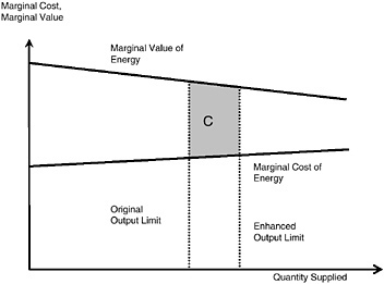
FIGURE 3-6 Benefits of resource supply enhancement.
A simple numerical example can be presented here as well. Assume that as a result of a supply enhancement program, additional oil could be produced at a cost of $25 per barrel and that the import price of oil was $40 per barrel. Assume that the import price would not change as a result of the increase in oil production. Assume that the enhancement could increase the production rate by 100,000 barrels per day. Then the net benefits of that program would be 36.5 million barrels, multiplied by $15 per barrel, for a total benefit of $547 million.
There is a second potential component to the net economic benefit resulting from resource supply enhancement. This second component is based on induced changes in energy or other markets throughout the economy. Increases in the supply of natural gas, oil reserves, or other resource stocks can lead to changes in their prices. Here, too, a reasonable simplifying approximation is that these changes in no way change the economic benefits.
A price decrease would make the sellers of the particular commodity financially worse off but would make the buyers of the commodity financially better off by the same amount. Just as in the case of energy efficiency enhancement, such price changes lead to no changes in net benefits and therefore can be disregarded for the calculation of net benefits.
Likewise, induced changes in supply and demand quantities throughout the rest of the economy can be expected to lead to very small, if any, changes in net benefits, as long as the markets being considered are competitive. The reason for this is exactly the same as discussed above for energy efficiency enhancement: In a perfectly competitive market, the marginal cost of producing more of a commodity will be equal to the price of that commodity, and the marginal value to the user of the commodity will also be equal to its price. Therefore, the additional cost of producing more units will be exactly equal to the additional value to the economy of the additional units. The net between additional value and additional cost would be just zero.
Alternatively, for resource supply enhancements, one could use a large-scale general equilibrium model of the economy if that model incorporated all of the important divergences from perfect competition and all of the other tax or institutional distortions. The same considerations outlined for Figure 3-6 would be important here as well.
Terms-of-Trade Impacts
Some technology changes would lead to reductions in imports of energy commodities or other commodities. These reductions might change the unit prices that the United States pays for such commodities. Such changes are generally referred to as changes in the terms of trade. Reductions in the cost of imported commodities relative to the overall price level provide gains to the United States and corresponding losses to the countries that export the commodities to the United States. The economic benefit of these changes to the United States can easily be added to the benefits discussed above.20
Terms-of-trade benefits are calculated as shown in Figure 3-4, except that the relevant quantity is the amount of the commodity that is imported. The primary terms-of-trade benefit is just equal to the amount of the commodity imported multiplied by the reduction in the price of that imported commodity. That amount corresponds to area A in Figure 3-4. There is also a second benefit, equal to area B, calculated as one-half of the increase in quantity imported induced by the price increase21 multiplied by the reduction in the price of the imported commodity. However, this component is normally tiny in comparison to the primary component and can be ignored with no significant loss of accuracy.
For example, assume that the United States had been importing 9 million barrels per day of oil and that as a result of an energy technology advance, it would be importing only 8 million barrels per day. Assume further that that reduction in imports of oil to the United States would reduce the price of imported oil by $0.10 per barrel. Then, the largest component of the annual terms-of-trade benefits to the United States (area A) would be the product of 8 million barrels per day, 365 days per year, and $0.10 per barrel, or $292 million.
Assume further that the reduction in the oil price increased the importation of oil by 4,000 barrels of oil per day, so that the net reduction in oil imports would be 996,000 barrels of oil per day. Then, the second component, area B, would be equal to the product of one-half of 4,000 barrels per day, 365 days per year, and $0.10 per barrel, an additional benefit of $73,000 per year. This figure of $73,000 per year is small enough that it can be ignored without harming the accuracy of the calculation.
The Use of NEMS and Other Models
Instead of using the simplified computation discussed above, one could use a large-scale general equilibrium model of the economy that incorporated all of the important divergences from perfect competition and all of the various tax or other institutional distortions. However, it is dubious whether any of the existing models have all those capabilities. Moreover, even if the models had such complete capabilities, using them in a continuing process of benefit calculation would be extremely difficult, if not impossible.
NEMS is one such general equilibrium model, used by the Department of Energy in putting together its annual Gov-
ernment Performance and Results Act (GPRA) submission (NREL, 2004). It can be used to generate input data for subsequent use in calculating benefits in a reduced forms model.
The relatively simple calculating procedures outlined above require future projections of basic energy information, in particular of supply and demand for various forms of energy and of marginal costs and/or prices. Such basic information generally can be developed only with a coherent model that projects possible equilibrium conditions for future years. Internal consistency among price and quantity projections for a given scenario, and between scenarios, normally requires use of a coherent model of the energy system. The committee believes that NEMS does provide such projections of prices, marginal costs, and supply/demand quantities.
Developing these net benefit calculations will therefore rely on the use of NEMS only indirectly, through its internally consistent projections of prices, marginal cost, and supply/demand quantities. The procedures recommended by the committee do not anticipate use of the NEMS directly to calculate net benefits. Such procedures can easily be implemented using simple spreadsheets, with particular parameters (such as projections of prices, marginal costs, and supply/demand quantities) taken from a NEMS equilibrium.
Several other calculating procedures, while superficially useful for estimating benefits, are not appropriate for the measurement of economic benefits and should not be used as net benefit estimates when estimating energy efficiency advances: (1) net change in the cost of particular energy commodities for individuals or groups of energy users, (2) net change in the per unit cost of energy commodities for individuals or groups of energy users, or (3) the aggregate change in the total use of energy.
One could measure for individuals or groups of energy users the net change in the cost of particular energy commodities resulting in energy efficiency advances. Note that this measure does not correspond with the impacts diagrammed in Figures 3-4 through 3-6. A simple example illustrates the fallacy. Assume that the elasticity of demand for energy is −1.0, so that a 10 percent reduction in the marginal cost of energy services would lead to a 10 percent increase in the use of such energy services. In that case, in response to a 10 percent reduction in the average or marginal cost of energy services, the energy use would increase by 10 percent, leaving unchanged the product of average cost and usage quantity. But because the product of average cost and usage quantity is simply the total cost of purchasing the energy services, the total cost of purchasing energy services would not change in response to a decrease in the marginal cost or average cost of energy services.
Similarly, the total cost of purchasing energy services would not change in response to an increase in the marginal cost of energy services. However as Figures 3-4 to 3-6 have illustrated, any and all such reductions in the average cost of energy services stemming from energy efficiency advances would have positive net benefits. Thus the first measure—the net change in the cost of particular energy commodities resulting in energy efficiency advances—is not an appropriate measure of net benefits.22
One can illustrate this with the numerical examples given for the lighting program. In the initial situation, total energy services would be 5,475 trillion lumen-hours at a cost of $0.0000008 per lumen-hour, or $4.60 billion. After the increase in efficiency of the lights, consumers would use 6,022 trillion lumen-hours of energy services at a cost of $0.0000004 per lumen-hour, or $2.41 billion. This would give an estimate of benefits equal to $2.19 billion, in contrast to the actual benefits of $2.30 billion.
In a situation where the consumer price exceeds the marginal cost of energy, the error would be greater. Here we assume that the consumer pays a price of $0.12 per kilowatt-hour. In the initial situation, total energy service would be 5,475 trillion lumen-hours of energy services at a cost of $0.0000024 per lumen-hour, or $13.14 billion. After the increase in efficiency of the lights, consumers would use 6,022 trillion lumen-hours of energy services at a consumer cost of $0.0000012 per lumen-hour, or $7.22 billion. If one were to calculate the benefits based on the cost paid by the consumer, the estimate would be equal to $5.92 billion, in contrast to the actual benefits of $2.96 billion. More appropriately, if one were to calculate the benefits based on the total cost of energy to society, a cost of energy of $0.04 per kilowatt-hour would give an estimate of benefits equal to $2.19 billion (exactly as calculated above), in contrast to the actual benefits of $2.96 billion.
The second measure—net change in the per unit cost of energy commodities for individuals or groups of energy users—is also an inappropriate measure of net benefits. These changes in the per unit cost of energy commodities typically are simply the result of price changes. But such price changes lead to benefits for the some members of the economy and equal but opposite net benefits for other members. Summed over all members of the economy, such price changes lead to no net benefits, so the per unit cost of energy commodities is not an appropriate measure of net benefits.
The third measure, the aggregate change in the total use of energy, is also inappropriate. As shown above, if the marginal cost of energy commodities is less than the marginal value of those commodities, increases in the total use of those energy commodities would lead to increases in net benefits. On the other hand, if the marginal cost of energy commodities is above their marginal value, increases in the total use of those energy commodities would lead to reductions in net benefits. Therefore, measurements of the total use of energy commodities will not provide a good measure of net economic benefits.


