
CHAPTER SIX
Changes in the Climate System
Scientific understanding of the factors and processes that govern the evolution of Earth’s climate has increased markedly over the past several decades, as has the ability to simulate and project future changes in the climate system. As noted in Chapter 2, this knowledge has been regularly assessed, synthesized, and summarized by the Intergovernmental Panel on Climate Change (IPCC), the U.S. Global Climate Research Program (USGCRP, referred to as the U.S. Climate Change Science Program from 2000 to 2008), and other groups to provide a thorough and detailed description of what is known about past, present, and projected future changes in climate and related human and environmental systems. This chapter provides an updated overview of the current state of knowledge about the climate system, followed by a list of some of the key scientific advances needed to further improve our understanding.
To help frame the sections that follow, it is useful to consider some questions that decision makers are asking or will be asking about changes in the climate system:
-
How are temperature and other aspects of climate changing?
-
How do we know that humans are responsible for these changes?
-
How will temperature, precipitation, severe weather, and other aspects of climate change in my city/state/region over the next several decades?
-
Will these changes be steady and gradual, or abrupt?
-
Will seasonal and interannual climate variations, like El Niño events, continue the same way or will they be different?
-
Why is there so much uncertainty about future changes?
This chapter attempts to answer these questions or explain what additional research would be needed to answer them. The chapters that follow focus on the impacts of climate change on a range of human and environmental systems, the role of these systems in driving climate change, and the state of scientific knowledge regarding actions that could potentially be taken to adapt to or limit the magnitude of climate change in those systems. All of the chapters in Part II follow a similar structure and are more detailed and extensively referenced than the concise overview of climate change science found in Chapter 2. However, these chapters represent only highlights of a broad and extensive collection of scientific research; readers desiring further detail are encouraged to consult other recent assessment reports and the primary literature.
FACTORS INFLUENCING EARTH’S CLIMATE
The Greenhouse Effect
The Earth’s physical climate system, which includes the atmosphere, oceans, cryosphere, and land surface, is complex and constantly evolving. Nevertheless, the laws of physics, chemistry, and biology ultimately govern the system and can be used to understand how and why climate varies from place to place and over time. For example, the energy balance of the Earth as a whole is determined by the difference between incoming and outgoing energies at the top of the atmosphere. The only significant incoming energy is radiation from the sun, which is concentrated at short wavelengths (visible and ultraviolet light), while the outgoing energy includes both infrared (long-wavelength) radiation emitted by the Earth and the portion of incoming solar radiation (about 30 percent on average) that is reflected back to space by clouds, small particles in the atmosphere, and the Earth’s surface. If the outgoing energy is slightly lower than the incoming energy for a period of time, then the climate system as a whole will warm until the outgoing radiation from the Earth balances the incoming radiation from the sun.
The temperature of the Earth’s surface and lower atmosphere depends on a broader range of factors, but the transfer of radiation again plays an important role, as does the composition of the atmosphere itself. Nitrogen (N2) and oxygen (O2) make up most of the atmosphere, but these gases have almost no effect on either the incoming radiation from the sun or the outgoing radiation emitted by the Earth’s surface. Certain other gases, however, absorb and reemit the infrared radiation emitted by the surface, effectively trapping heat in the lower atmosphere and keeping the Earth’s surface much warmer—roughly 59°F (33°C) warmer—than it would be if greenhouse gases were not present.1 This is called the greenhouse effect, and the gases that cause it—including water vapor, carbon dioxide (CO2), methane (CH4), and nitrous oxide (N2O)—are called greenhouse gases (GHGs). GHGs only constitute a small fraction of the Earth’s atmosphere, but even relatively small increases in the amount of these gases in the atmosphere can amplify the natural greenhouse effect, warming the Earth’s surface (see Figure 2.1).
Carbon Dioxide
The important role played by CO2 in the Earth’s energy balance has been appreciated since the late 19th century, when Swedish scientist Svante Arrhenius first proposed a link between CO2 levels and temperature. At that time, humans were only beginning to burn fossil fuels—which include coal, oil, and natural gas—on a wide scale for energy. The combustion of these fuels, or any material of organic origin, yields mostly CO2 and water vapor, but also small amounts of other by-products, such as soot, carbon monoxide, sulfur dioxide, and nitrogen oxides. All of these substances occur naturally in the atmosphere, and natural fluxes of water and CO2 between the atmosphere, oceans, and land surface play a critical role in both the physical climate system and the Earth’s biosphere. However, unlike water vapor molecules, which typically remain in the lower atmosphere for only a few days before they are returned to the surface in the form of precipitation, CO2 molecules are only exchanged slowly with the surface. The excess CO2 emitted by fossil fuel burning and other human activities will thus remain in the atmosphere for many centuries before it can be removed by natural processes (Solomon et al., 2009).
A number of agencies and groups around the world, including the Carbon Dioxide Information Analysis Center at Oak Ridge National Laboratory and the International Energy Agency, produce estimates of how much CO2 is released to the atmosphere every year by human activities. The most recent available estimates indicate that, in 2008, human activities released over 36 Gt (gigatons, or billion metric tons) of CO2 into the atmosphere—including 30.6 ± 1.7 Gt from fossil fuel burning, plus an additional 4.4 ± 2.6 Gt from land use changes and 1.3 ± 0.1 Gt from cement production (Le Quéré et al., 2009). Emissions from fossil fuels have increased sharply over the last two decades, rising 41 percent since 1990 (Figure 6.1). CO2 emissions due to land use change—which are dominated by tropical deforestation—are estimated based on a variety of methods and data sources, and the resulting estimates are both more uncertain and more variable from year-to-year than fossil fuel emissions. Over the past decade (2000–2008), Le Quéré et al. (2009) estimate that land use changes released 5.1 ± 2.6 Gt of CO2 each year, while fossil fuel burning and cement production together released on average 28.2 ± 1.7 Gt of CO2 per year.
Up until the 1950s, most scientists thought the world’s oceans would simply absorb most of the excess CO2 released by human activities. Then, in a series of papers in the late 1950s (e.g., Revelle and Suess, 1957), American oceanographer Roger Revelle and several collaborators hypothesized that the world’s oceans could not absorb all the excess CO2 being released from fossil fuel burning. To test this hypothesis, Revelle’s colleague C. D. Keeling began collecting canisters of air at the Mauna Loa Observatory
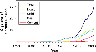
FIGURE 6.1 Estimated global CO2 emissions from fossil fuel sources, in gigatons (or billion metric tons). Based on data from Boden et al. (2009; available at http://cdiac.ornl.gov/trends/emis/tre_glob.html).
in Hawaii, far away from major industrial and population centers, and analyzing the composition of these samples to determine whether CO2 levels in the atmosphere were increasing. Similar in situ measurements continue to this day at Mauna Loa as well as at many other sites around the world. The resulting high-resolution, well-calibrated, 50-year-plus time series of highly accurate and precise atmospheric CO2 measurements (Figure 6.2), commonly referred to as the Keeling curve, is both a major scientific achievement and a key data set for understanding climate change.
The Keeling curve shows that atmospheric CO2 levels have risen by more than 20 percent since 1958; as of January 2010, they stood at roughly 388 ppm, rising at an average annual rate of almost 2.0 ppm per year over the past decade (Blasing, 2008; Tans, 2010). When multiplied by the mass of the Earth’s atmosphere, this increase corresponds to 15.0 ± 0.1 Gt CO2 added to the atmosphere each year, or roughly 45 percent of the excess CO2 released by human activities over the last decade. The remaining 55 percent is absorbed by the oceans and the land surface. The size of these CO2 “sinks” is estimated via both modeling and direct observations of CO2 uptake in the oceans and on land. These estimates indicate that the oceans absorbed on average 8.4 ± 1.5 Gt CO2 annually over the last decade (or 26 percent of human emissions), while the land surface took up 11.0 ± 3.3 Gt per year (29 percent), with a small residual of 0.3 Gt (Le Quéré et al., 2009).
A careful examination of the Keeling curve reveals that atmospheric CO2 concentrations are currently increasing twice as fast as they did during the first decade of the record (compare the slope of the black line in Figure 6.2). This acceleration in the rate of CO2 rise can be attributed in part to the increases in CO2 emissions due to increasing
![FIGURE 6.2 Atmospheric CO2 concentrations (in parts per million [ppm]) at Mauna Loa Observatory in Hawaii. The red curve, which represents the monthly averaged data, includes a seasonal cycle associated with regular changes in the photosynthetic activity in plants, which are more widespread in the Northern Hemisphere. The black curve, which represents the monthly averaged data with the seasonal cycle removed, shows a clear upward trend. SOURCE: Tans (2010; available at http://www.esrl.noaa.gov/gmd/ccgg/trends/).](/openbook/12782/xhtml/images/p2001c3c5g187001.jpg)
FIGURE 6.2 Atmospheric CO2 concentrations (in parts per million [ppm]) at Mauna Loa Observatory in Hawaii. The red curve, which represents the monthly averaged data, includes a seasonal cycle associated with regular changes in the photosynthetic activity in plants, which are more widespread in the Northern Hemisphere. The black curve, which represents the monthly averaged data with the seasonal cycle removed, shows a clear upward trend. SOURCE: Tans (2010; available at http://www.esrl.noaa.gov/gmd/ccgg/trends/).
energy use and development worldwide (as indicated in Figure 6.1). However, recent studies suggest that the rate at which CO2 is removed from the atmosphere by ocean and land sinks may also be declining (Canadell et al., 2007; Khatiwala et al., 2009). The reasons for this decline are not well understood, but, if it continues, atmospheric CO2 concentrations would rise even more sharply, even if global CO2 emissions remain the same. Improving our understanding and estimates of current and projected future fluxes of CO2 to and from the Earth’s surface, both over the oceans and on land, is a key research need (research needs are discussed at the end of the chapter).
To determine how CO2 levels varied prior to direct atmospheric measurements, scientists have studied the composition of air bubbles trapped in ice cores extracted from the Greenland and Antarctic ice sheets. These remarkable data, though not as accurate and precise as the Keeling curve, show that CO2 levels were relatively constant for thousands of years preceding the Industrial Revolution, varying in a narrow band between 265 and 280 ppm, before rising sharply starting in the late 19th century (Figure 6.3). The current CO2 level of 388 ppm is thus almost 40 percent higher Scripps Institution of Oceanography
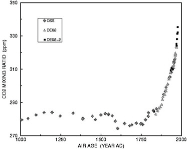
FIGURE 6.3 CO2 variations during the last 1,000 years, in parts per million (ppm), obtained from analysis of air bubbles trapped in an ice core extracted from Law Dome in Antarctica. The data show a sharp rise in atmospheric CO2 starting in the late 19th century, coincident with the sharp rise in CO2 emissions illustrated in Figure 6.1. Similar data from other ice cores indicate that CO2 levels remained between 260 and 285 ppm for the last 10,000 years. SOURCE: Etheridge et al. (1996).
than preindustrial conditions (usually taken as 280 ppm). As discussed in further detail in the next section, data from even longer ice cores extracted from the hearts of the Greenland and Antarctic ice sheets—the bottoms of which contain ice that was formed hundreds of thousands of years ago—indicate that the current CO2 levels are higher than they have been for at least 800,000 years.
Collectively, the in situ measurements of CO2 over the past several decades, ice core measurements showing a sharp rise in CO2 since the Industrial Revolution, and detailed estimates of CO2 sources and sinks provide compelling evidence that CO2 levels are increasing as a result of human activities. There is, however, an additional piece of evidence that makes the human origin of elevated CO2 virtually certain: measurements of the isotopic abundances of the CO2 molecules in the atmosphere—a chemical property that varies depending on the source of the CO2—indicate that most of the excess CO2 in the atmosphere originated from sources that are millions of years old. The only source of such large amounts of “fossil” carbon are coal, oil, and natural gas (Keeling et al., 2005).
Climate Forcing
Changes in the radiative balance of the Earth—including the enhanced greenhouse effect associated with rising atmospheric CO2 concentrations—are referred to as climate forcings (NRC, 2005d). Climate forcings are estimated by performing detailed calculations of how the presence of a forcing agent, such as excess CO2 from human activities, affects the transfer of radiation through the Earth’s atmosphere.2 Climate forcings are typically expressed in Watts per square meter (W/m2, or energy per unit area), with positive forcings representing warming, and are typically reported as the change in forcing since the start of the Industrial Revolution (usually taken to be the year 1750). Figure 6.4 provides a graphical depiction of the estimated globally averaged strength of the most important forcing agents for recent climate change. Each of these forcing agents are discussed below.
Well-Mixed Greenhouse Gases
Carbon dioxide (CO2). The CO2 emitted by human activities is the largest single climate forcing agent, accounting for more than half of the total positive forcing since 1750 (see Figure 6.4). As of the end of 2005, the forcing associated with human-induced atmospheric CO2 increases stood at 1.66 ± 0.17 W/m2 (Forster et al., 2007). This number may seem small relative to the total energy received by the Earth from the sun (which averages 342 W/m2, of which 237 W/m2 is absorbed by the Earth system, after accounting for reflection of 30 percent of the solar energy back to space). When multiplied by the surface area of the Earth, however, the CO2 forcing is roughly 850 terawatts, which is more than 50 times the total power consumed by all human activities.
Human activities have also led to increases in the concentrations of a number of other “well-mixed” GHGs—those that are relatively evenly distributed because their molecules remain in the atmosphere for at least several years on average. Many of these gases are much more potent warming agents, on a molecule-for-molecule basis, than CO2, so even small changes in their concentrations can have a substantial influence. Collectively, they produce an additional positive forcing (warming) of 1.0 ± 0.1 W/m2, for a total well-mixed GHG-induced forcing (including CO2) of 2.63 ± 0.26 W/m2
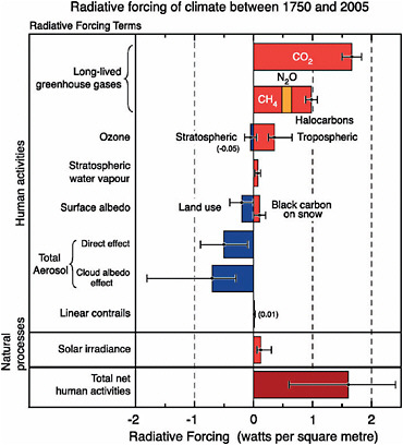
FIGURE 6.4 Radiative forcing of climate between 1750 and 2005 due to both human activities and natural processes, expressed in Watts per square meter (energy per unit area). Positive values correspond to warming. See text for details. SOURCE: Forster et al. (2007).
(Forster et al., 2007) (see Figure 6.4). Forcing estimates for all of the well-mixed GHGs are quite accurate because we have precise measurements of their concentrations, their influence on the transfer of radiation through the atmosphere is well understood, and they become relatively evenly distributed across the global atmosphere within a year or so of being emitted.
Methane (CH4). Methane is produced from a wide range of human activities, including natural gas management, fossil fuel and biomass burning, animal husbandry, rice cultivation, and waste management (Houweling et al., 2006). Natural sources of CH4—which are smaller than human sources—include wetlands and termites, and both of
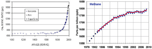
FIGURE 6.5 Atmospheric CH4 concentrations in parts per billion (ppb), (left) during the past millennium, as measured in Antarctic ice cores, and (right) since 1979, based on direct atmospheric measurements. SOURCES: Etheridge et al. (2002) and NOAA/ESRL (2009).
these sources are actually influenced to some degree by changes in land use. Recent measurements have suggested that plants and crops may also emit trace amounts of CH4 (Keppler et al., 2006), although the size of this source has been questioned (Dueck et al., 2007).
The atmospheric concentration of CH4 rose sharply through the late 1970s before starting to level off, ultimately reaching a relatively steady concentration of around 1775 ppb—which is more than two-and-a-half times its average preindustrial concentration—from 1999 to 2006 (Figure 6.5). There have been several theories proposed for the apparent leveling off of CH4 concentrations, including a decline in industrial emissions during the 1990s and a slowdown of natural wetland-related emissions (Dlugokencky et al., 2003). As discussed at the end of the chapter, there are also concerns that warming temperatures could lead to renewed rise in CH4 levels as a result of melting permafrost across the Arctic (Schuur et al., 2009) or, less likely, the destabilization of methane hydrates3 on the seafloor (Archer and Buffet, 2005; Overpeck and Cole, 2006). The causes of the recent uptick in concentrations in 2007 and 2008 are currently being studied (Dlugokencky et al., 2009).
Unlike CO2, which is only removed slowly from the atmosphere by processes at the land surface, the atmospheric concentration of CH4 is limited mainly by a chemical reaction in the atmosphere that yields CO2 and water vapor. As a result, molecules of CH4 spend on average less than 10 years in the atmosphere. However, CH4 is a much
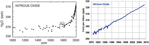
FIGURE 6.6 N2O concentrations in the atmosphere, in parts per billion (ppb), (left) during the last millennium, and (right) since 1979. SOURCES: Etheridge et al. (1996) and NOAA/ESRL (2009).
more potent warming agent, on a molecule-for-molecule basis,4 than CO2, and its relative concentration in the atmosphere has risen by almost four times as much as CO2. Hence, the increases in CH4 since 1750 are associated with a climate forcing of roughly 0.48 ± 0.05 W/m2 (Forster et al., 2007), or around 18 percent of the total forcing by well-mixed GHGs.
Nitrous oxide (N2O). Concentrations of nitrous oxide in the atmosphere have increased around 15 percent since 1750, primarily as a result of agricultural activities (especially the application of chemical fertilizers) but also as a by-product of fossil fuel combustion and certain industrial process. The average atmospheric concentration of N2O continues to grow at a steady rate of around 0.8 ppb per year and, as of the end of 2008, stood at just over 322 ppb (Figure 6.6) (see also NASA, 2008). N2O is an extremely potent warming agent—more than 300 times as potent as CO2 on a molecule-by-molecule basis—and its molecules remain in the atmosphere more than 100 years on average. Thus, even though N2O concentrations have not increased nearly as much since 1750 as CH4 or CO2, N2O still contributes a climate forcing of 0.16 ± 0.02 W/m2 (Forster et al., 2007), or around 6 percent of total well-mixed GHG forcing. N2O and its decomposition in the atmosphere also have a number of other environmental effects—for example, N2O is now the most important stratospheric ozone-depleting substance being emitted by human activities (Ravishankara et al., 2009).
Halogenated gases. Over a dozen halogenated gases, a category that includes ozone-depleting substances such as chlorofluorocarbons (CFCs), hydrofluorocarbons, per-
fluorocarbons, and sulfur hexafluoride, also contribute to the positive climate forcing associated with well-mixed GHGs. Although relatively rare—their concentrations are typically measured in parts per trillion—many of the halogenated gases have very long residence times in the atmosphere and are extremely potent forcing agents on a molecule-by-molecule basis (Ravishankara et al., 1993). Collectively they contribute an additional 0.33 ± 0.03 W/m2 of climate forcing. Most halogenated gases do not have any natural sources (see, e.g., Frische et al., 2006) but rather arise from a variety of industrial activities. Emissions of many of these ozone-depleting compounds have declined sharply over the past 15 years because of the Montreal Protocol (see below). As a result, their atmospheric concentrations, and hence climate forcing, are now declining slightly each year as they are slowly removed from the atmosphere by natural processes (Figure 6.7) (NASA, 2008). It has been estimated that the forcing associated with halogenated gases would be 0.2 W/m2 higher than it is today if emissions reductions due to the Montreal Protocol had not taken place (Velders et al., 2007; see also Chapter 17).
Other Greenhouse Gases
Ozone (O3). Ozone plays a number of important roles in the atmosphere, depending on location, and its concentration varies substantially, both vertically and horizontally. The highest concentrations of ozone are found in the stratosphere—the layer of the atmosphere extending from roughly 10 to 32 miles (15 to 50 km) in height (Figure 6.8)—where it is produced naturally by the dissociation of oxygen molecules by ultraviolet light. This chemical reaction, along with the photodissociation of ozone itself, plays the beneficial role of absorbing the vast majority of incoming ultraviolet radiation, which is harmful to most forms of life, before it reaches the Earth’s surface. Levels of ozone in the stratosphere have been declining over the past several decades, especially over Antarctica. Scientific research has definitively shown that CFCs, along with a few other related man-made halogenated gases (see above), are responsible for these ozone losses in the stratosphere; thus, halogenated gases contribute to both global warming and stratospheric ozone depletion. The Montreal Protocol, which was originally signed in 1987 and has now been revised several times and ratified by 196 countries, has resulted in a rapid phase-out of these gases (see Figure 6.7). Recent evidence suggests that ozone levels in the stratosphere are starting to recover as a result, although it may be several more decades before the ozone layer recovers completely (CCSP, 2008a).
Near the Earth’s surface, ozone is considered a pollutant, causing damage to plants and animals, including humans, and it is one of the main components of smog (see Chapter 11). Most surface ozone is formed primarily when sunlight strikes air that
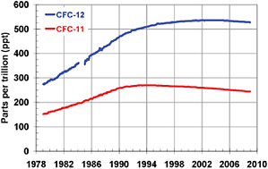
FIGURE 6.7 Atmospheric concentrations of the two halogenated gases with the largest individual climate forcings, CFC-11 and CFC-12, from 1979 to 2008. The Montreal Protocol limited the production of these and other compounds, and so their atmospheric concentrations are now slowly declining. SOURCE: NOAA/ESRL (2009).
contains nitrogen oxides (NOx) in combination with carbon monoxide (CO) or certain volatile organic compounds (VOCs). All of these substances have natural sources, but their concentrations have increased as a result of human activities. Much of the NOx and CO in the troposphere comes from man-made sources that involve burning, including automobile exhaust and power plants, while sources of VOCs include vegetation, automobiles, and certain industrial activities.
Ozone is also found in the upper troposphere, where its sources include local formation, horizontal and vertical mixing processes, and downward transport from the stratosphere. In general, tropospheric ozone levels show a lot of variability in both space and time, and there are only a few locations with long-term records, so it is difficult to estimate long-term ozone trends. Observational evidence to date shows increases in ozone in various parts of the world (e.g., Cooper et al., 2010). Models that include explicit representations of atmospheric chemistry and transport have also been used to estimate long-term ozone trends. These models, which are generally able to simulate observed ozone changes, indicate that tropospheric ozone levels have increased appreciably during the 20th century (Forster et al., 2007).
In addition to its role in near-surface air pollution and absorbing ultraviolet radiation in the stratosphere, ozone is a GHG, and so changes in its concentration yield a climate forcing. The losses of ozone in the stratosphere are estimated to yield a small negative forcing (cooling) of −00.05 ± 0.10W/m2, while increases in tropospheric ozone, which
FIGURE 6.8 The vertical distribution of ozone with height, showing the protective layer of ultraviolet-absorbing ozone in the stratosphere, the harmful ozone (smog) near the Earth’s surface, and the lesser—but still important—amounts of ozone in the upper troposphere. SOURCE: UNEP et al. (1994).
are comparatively larger, are estimated to yield a positive forcing of between 0.25 and 0.65 W/m2, with a best estimate of 0.35 W/m2 (Forster et al., 2007) (see Figure 6.4). Thus, in total, the changes in atmospheric ozone are responsible for a positive forcing that is on par with the halogenated gases and possibly as large as or slightly larger than the forcing associated with CH4. However, the exact ozone forcing is more uncertain than for the well-mixed GHGs.
Water vapor (H2O). Water vapor is technically the most abundant GHG and also the most important in terms of its contribution to the natural greenhouse effect (see Figure 2.1). A number of human activities (primarily agricultural irrigation but also through cooling towers, aircraft exhaust, and other sources) can influence local water vapor levels. However, on a global basis the concentration of water vapor in the lower atmosphere is controlled by the rate of evaporation and precipitation, which are processes that occur on a relatively fast time scale and are much more strongly influenced by changes in atmospheric temperature and circulation than by human activities directly. Thus, water vapor is usually considered to be part of the climate system—and indeed, it is involved in a number of important climate feedback processes, as described below—rather than a climate forcing agent.
In the stratosphere, on the other hand, water vapor is relatively rare and somewhat isolated from the hydrological cycle in the lower atmosphere. Processes that influence water vapor concentrations at these high altitudes can thus lead to a small but discernible climate forcing. The largest such forcing is associated with the oxidation of CH4 into water vapor and CO2: as CH4 concentrations have increased, so has this source of water vapor in the stratosphere, leading to a small positive climate forcing estimated to be 0.05 ± 0.05 W/m2 (Hansen et al., 2005).5 Recent satellite-based observations reveal that stratospheric water vapor levels have actually declined since 2000 (Solomon et al., 2010); the causes and possible implications of this decline are still being studied.
Other Climate Forcing Agents
Aerosols. Small liquid or solid particles suspended in the atmosphere—aerosols—can be composed of many different chemicals, come from many different sources (including both natural sources and human activities), and have a wide range of effects. Fossil fuel burning, industrial activities, land use change, and other human activities have generally increased the number of aerosol particles in the atmosphere, especially over and downwind of industrialized counties. The net climate forcing associated with aerosols is estimated to be −11.2W/m2 (Forster et al., 2007; see also Murphy et al., 2009), which offsets roughly one-third of the total positive forcing associated with human emissions of GHGs (see Figure 6.4). However, the forcing associated with aerosols is more uncertain than the forcing associated with GHGs, in part because the global distribution and composition of aerosols are not very well known and in part because of the diversity and complexity of aerosol radiative effects.
Two separate types of effects contribute to the net cooling associated with aerosols: (1) a “direct effect,” which occurs because most aerosols scatter a portion of the incoming sunlight that strikes them back to space, and (2) “indirect effects,” which arise because aerosols play an important role in the formation and properties of cloud droplets, and on average the increasing number of aerosols have caused clouds to reflect more sunlight back to space. Certain kinds of aerosols, including dust particles
and black carbon (soot), absorb both incoming solar energy and the outgoing infrared energy emitted by the Earth. These aerosols tend to warm the atmosphere, offsetting some (but not all) of the cooling associated with the direct and indirect effects. Black carbon particles that settle on snow and ice surfaces can also accelerate melting; however, this positive forcing is typically included in estimates of the forcing associated with land use change, which is discussed below.
It is worth noting the sources of a few key types of aerosols to illustrate their diversity: Dust and some organic aerosols arise from natural processes, but some human activities such as land use change also lead to changes in the abundance of these species. Black carbon particles are produced from the burning of both fossil fuels and vegetation. Sulfate (SO4) aerosols—which are a major contributor to the aerosol direct and indirect effects—have three notable sources: fossil fuel burning, marine phytoplankton, and volcanoes. The composition and size of each of these aerosol species affect how they absorb or scatter radiation, how much water vapor they absorb, how effectively they act to form cloud droplets, and how long they reside in the atmosphere—although in general most aerosols only remain in the atmosphere for a few weeks on average.
In addition to their role in global climate forcing, aerosols also have a number of other important environmental effects. The same industrial emissions that give rise to SO4 aerosols also contribute to acid rain, which has a major detrimental effect on certain ecosystems. One of the major objectives—and successes—of the 1990 Clean Air Act (P.L. 101-549) was to reduce the amount of sulfur emissions in the United States. Similar laws in Europe have also been successful in reducing SO4 aerosol concentrations (Saltman et al., 2005). The relationship between aerosols and cloud formation also means that changes in aerosols play an important role in modulating precipitation processes (see Chapters 8 and 15). Also, many aerosols are associated with negative impacts on public health, as discussed in further detail in Chapter 11.
Finally, aerosol emissions represent an important dilemma facing policy makers trying to limit the magnitude of future climate change: If aerosol emissions are reduced for health reasons, or as a result of actions taken to reduce GHG emissions, the net negative climate forcing associated with aerosols would decline much more rapidly than the positive forcing associated with GHGs due to the much shorter atmospheric lifetime of aerosols, and this could potentially lead to a rapid acceleration of global warming (see, e.g., Arneth et al., 2009). Understanding the many and diverse effects of aerosols is also important for helping policy makers evaluate proposals to artificially increase the amount of aerosols in the stratosphere in an attempt to offset global warming (see Chapter 15).
Changes in land cover and land use. Human modifications of the land surface can have a strong local or even regional effect on climate. One notable example is the “urban heat island” effect on temperatures, described below and in Chapter 12. Globally, land cover and land use changes are important sources of several GHGs, such as the release of CO2 from deforestation or CH4 from rice paddies. Land use and land cover change can also yield a global climate forcing by altering the reflectivity of the Earth’s surface—for example, by replacing forests (which absorb most incident sunlight) with cropland (which is generally somewhat more reflective). Satellite measurements provide an excellent record of how changes in land cover have influenced surface reflectivity over the last few decades, although in some cases there is uncertainty as to whether observed changes are directly human-induced, part of a feedback process, or attributable to natural changes. To estimate global patterns of land use change for the last several hundred years, scientists use historical and paleoecological records combined with land use models that can simulate changes in vegetation over time in response to both climatic and nonclimatic effects.
Most recent published estimates of the global climate forcing associated with land use and land cover change are in the range of −00.1 o −00.3W/m2, although some estimates are as large as −00.5W/m2, while others indicate a small positive net forcing (Forster et al., 2007). As noted above, an additional land-surface effect is the deposition of black carbon aerosols (soot) on white snow and ice surfaces, which leads to melting and has been estimated to yield a positive forcing of up to 0.2 W/m2, although more recent estimates have suggested a somewhat smaller warming effect (Hansen et al., 2005). Thus, the total climate forcing associated with modifications to the land surface due to human activities since 1750 could potentially be positive or negative, but the balance of evidence seems to suggest a slight cooling effect.
Changes in solar radiation. As discussed in the next section, even small variations in the amount or distribution of energy received from the sun can have a major influence on Earth’s climate when they persist for many thousands of years. However, satellite measurements of solar output show no net increase in solar forcing over the last 30 years, only small periodic variations associated with the 11-year solar cycle (Figure 6.9). Changes in solar activity prior to the satellite era are estimated based on a variety of techniques including observations of sunspot numbers, which correspond roughly with solar output (Figure 6.10). The available evidence suggest that solar activity has been roughly constant (aside from the 11-year solar cycle) since the mid-20th century but that it increased slightly during the late 19th and early 20th centuries. The total solar forcing since 1750 is estimated to be less than 0.3 W/m2 (Forster et al., 2007).
Cosmic rays. Finally, it has been proposed that cosmic rays might influence Earth’s cli-
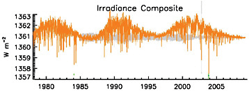
FIGURE 6.9 Solar irradiance observed at the top of the Earth’s atmosphere by satellites. There is no overall trend in irradiance since 1979, but the ~11-year solar cycle produces small variations in irradiance of roughly 1.5 W/m2. Due to the geometry of the Earth and the reflection of some of the incoming sunlight back to space, this 1.5 W/m2 variation in irradiance corresponds to a periodic oscillation in climate “forcing” of around 0.3 W/m2 (although climate forcing is usually defined as the overall change in forcing since 1750). SOURCE: Lean and Woods (in press).
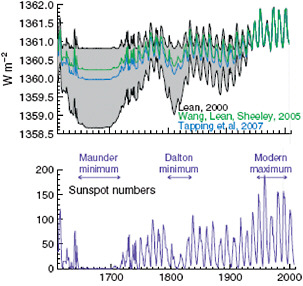
FIGURE 6.10 Estimated variations in solar irradiance at the top of the atmosphere by three different research teams during (top) the last 400 years based on (bottom) observations of sunspot numbers. All three irradiance reconstructions indicate drops in solar output during extended periods with low sunspot numbers, especially the Maunder and Dalton minimums (which are indicated in the bottom panel), and an increase in solar irradiance during the first several decades of the 20th century. The estimated total climate forcing associated with changes in solar irradiance since 1750 is 0.3 W/m2. (As noted in the caption for Figure 6.9, the climate forcing associated with solar irradiance changes must be scaled to account for Earth’s geometry and the reflection of some of the incident solar energy back to space.) SOURCE: Lean and Woods (in press).
mate by modifying cloud properties (Shaviv, 2002; Svensmark, 1998, 2006) or through a variety of other mechanisms (Gray et al., 2005). Cosmic rays are influenced by solar activity, so it is difficult to study the effect of cosmic rays in isolation. However, direct observations of cosmic ray fluxes do not show any net change over the last several decades (Benestad, 2005), and a plausible physical mechanism linking changes in cosmic rays to changes in climate has not been demonstrated. Hence, cosmic rays are not regarded as an important climate forcing (Forster et al., 2007).
Climate Feedbacks and Sensitivity
The influence of climate forcings on Earth’s temperature is modulated by the effects of feedbacks in the climate system. One example of a positive feedback is the ice-reflectivity feedback: If a positive climate forcing leads to a slight warming that melts ice, especially (white, highly reflective) sea ice floating on the (dark, highly absorptive) ocean surface, the surface of the Earth will reflect less sunlight back to space, and the increased absorption of solar radiation reinforces the initial warming. On the other hand, if warming were to cause an increase in the amount of low-lying clouds, which tend to cool the Earth by reflecting solar radiation back to space (especially when they occur over ocean areas), this would tend to offset some of the initial warming—a negative feedback. Other important feedbacks involve changes in evaporation, other kinds of clouds, land-surface properties, the vertical profile of temperature in the atmosphere, and the circulation of the atmosphere and oceans—all of which operate on different time scales and interact with one another and with other environmental changes in addition to responding directly to changes in temperature.
The net effect of all feedback processes determines the sensitivity of the climate system, or the response of the system to a given set of forcings (NRC, 2003b). Climate sensitivity is typically expressed as the temperature change expected if atmospheric CO2 levels were fixed at twice their preindustrial concentration, with all other forcings neglected (or 560 ppm of CO2, which corresponds to a climate forcing of 3.7 W/m2), and then remained there until the climate system reaches equilibrium. A variety of methods have been used to estimate climate sensitivity, including statistical analysis of climate forcing and observed temperature changes, analyses based on estimates of forcing and temperature variations from paleoclimatic records (see below), energy balance models, and climate models of varying complexity (e.g., Annan et al., 2005; Hegerl et al., 2006; Knutti et al., 2006; Murphy et al., 2004; Wigley et al., 2005). The IPCC’s latest comprehensive assessment of climate sensitivity based on these techniques indicates that the expected warming due to a doubling of CO2 is between 3.6°F and 8.1°F (2.0°C and 4.5°C), with a best estimate of 5.4°F (3.0°C) (Hegerl et al., 2007). Unfortunately, the
diversity and complexity of processes operating in the climate system mean that, even with continued progress in understanding climate feedbacks and monitoring global climate forcing and temperature changes, the exact sensitivity of the climate system may remain uncertain (Roe and Baker, 2007).
The concept of climate sensitivity technically only applies to equilibrium climate states, that is, the total warming after the oceans, cryosphere, and biosphere have had ample time to fully adjust to the imposed forcing. In reality, the strength of climate forcings and feedbacks are continuously varying, and it takes the climate system—especially the oceans—a long time to warm up in response to a positive climate forcing. In addition, many estimates of climate sensitivity do not include climate feedbacks associated with processes that operate on decadal to centennial time scales, such as the disappearance of glaciers, changes in vegetation distribution, or changes to the carbon cycle on land and in the oceans; several recent studies that consider some of these processes have suggested that Earth’s climate sensitivity may be substantially higher than the aforementioned “best estimate” (Hansen et al., 2008; Sokolov et al., 2009). Nevertheless, estimates of climate sensitivity are a useful metric for evaluating the causes of observed climate change and estimating how much the Earth will ultimately warm in response to past, present, and future human activities. Climate feedbacks and climate sensitivity also remain an important area for future research (see Research Needs at the end of this chapter).
OBSERVED CLIMATE CHANGE
Natural Climate Variability
Earth’s climate varies naturally on a wide range of time scales. Many of these variations are caused by complex interactions between the fast-moving, less-dense atmosphere and the more massive, slower-to-respond oceans. For example, the El Niño-Southern Oscillation (ENSO), which is caused by ocean-atmosphere interactions in the tropical Pacific Ocean, is a source of significant year-to-year variability around the world. The “warm” or “El Niño” phase is characterized by warmer-than-normal sea surface temperatures in the eastern equatorial Pacific. El Niño years are often associated with significant, predictable regional variations in temperature and rainfall across many remote parts of the world; in the United States, for example, El Niño years typically exhibit wetter-than-normal conditions in Southern California and the southern Great Plains. Global temperatures also tend to be slightly warmer during years with strong El Niño events, such as 1998, and slightly cooler during “cool” or “La Niña” years, such as 2008.
A multitude of other patterns of natural climate variability have also been identified, and many of these are associated with strong regional climate variations. Higher-latitude oscillations, such as the Northern and Southern Annular Modes (Thompson and Wallace, 2000, 2001), the Pacific Decadal Oscillation (Guan and Nigam, 2008; Mantua et al., 1997), the North Atlantic Oscillation, and the Atlantic Multidecadal Oscillation (Guan and Nigam, 2009), have a large influence on regional climate at decadal time scales, with impacts on, for example, salmon fisheries in the Pacific Northwest (Hare et al., 1999; Mantua and Hare, 2002) and the number of hurricanes making landfall in North America (Dailey et al., 2009). The exceptionally cold and snowy winter experienced on the East Coast of the United States during 2009-2010, which was balanced by warmer-than-normal temperatures in much of northeastern Canada and the high Arctic, can be attributed in part to a strong North Atlantic Oscillation event. Natural climate oscillations on multidecadal and longer time scales could also exist (e.g., Enfield et al., 2001; Schlesinger and Ramankutty,1994), though the instrumental record is too short and too sparse to unambiguously attribute their causal mechanisms (e.g., Zhang et al., 2007a).
Climate variations can also be forced by natural processes including volcanic eruptions, changes in the output from the sun, and changes in Earth’s orbit around the sun. Large, explosive volcanic eruptions, like Tambora in 1815, Krakatoa in 1883, El Chichón in 1983, and Pinatubo in 1991, spew copious amounts of sulfate aerosols into the stratosphere, cooling the Earth for several years (Briffa et al., 1998). The Pinatubo eruption is particularly noteworthy because it occurred in an era with widespread satellite and ground-based observations that allowed for the resulting aerosol distribution and climate response to be accurately quantified. These data indicate that aerosols induced a peak climate forcing of −22.5W/m2 several months after the Pinatubo eruption (Harries and Futyan, 2006) and that global surface temperatures dipped approximately 0.9°F (0.5°C) 2 years later, then recovered over the next several years as aerosol levels gradually declined (Trenberth and Dai, 2007). Data from Pinatubo and other volcanic eruptions have been used to estimate the strength of climate feedbacks that operate on relatively short time scales, such as the feedback associated with the correlation between temperature and water vapor in the atmosphere, and for calibrating and validating climate model results (e.g., Soden et al., 2002).
While there has not been a net increase in the Sun’s energy output over the past few decades (see Figure 6.9), the small variations in solar output associated with the 11-year solar cycle do lead to temperature and circulation change in the upper atmosphere (Shindell et al., 1999), may affect weather patterns in the tropical Pacific (Meehl et al., 2009a), and could potentially be associated with small variations in Earth’s average surface temperature (Camp and Tung, 2007; Lean and Woods, in press). There is
also evidence that changes in solar activity influence Earth’s climate on longer time scales. For example, the “Little Ice Age” (Matthes, 1939), a period with slightly cooler temperatures between the 17th and 19th centuries, may have been caused in part by a low solar activity phase from 1645 to 1715 called the Maunder Minimum (Eddy, 1976; Shindell et al., 2001) (see Figure 6.10). Estimates of variations in solar output on even longer time scales—going back thousands of years—have also been produced by analyzing cosmogenic isotopes in tree rings and ice cores (e.g., Weber et al., 2004). However, these estimates, and hence the extent of solar influence on global climate on these time scales, are even more uncertain (Lean and Woods, in press).
Perhaps the most dramatic example of natural climate variability is the Ice Age cycle (Figure 6.11). Detailed analyses of ocean sediments, ice cores, and other data (see, e.g.,
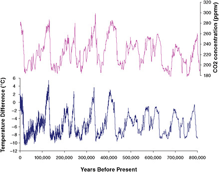
FIGURE 6.11 Analysis of ice core data extending back 800,000 years documents (top) the Earth’s changing CO2 concentration and (bottom) estimated temperatures in the Antarctic region. Until the past century, natural factors caused atmospheric CO2 concentrations to vary within a range of about 180 to 300 ppm. Note that time progresses from right to left in this figure, and that neither temperature changes nor the rapid CO2 rise (to 388 ppm) over the past century are shown. SOURCES: Based on data from (top) Lüthi et al. (2008) and (bottom) Jouzel et al. (2007). Data available at http://www.ncdc.noaa.gov/paleo/icecore/antarctica/domec/domec_epica_data.html.
Lüthi et al., 2008) show that for at least the past 800,000 years, and probably the past several million years, the Earth has gone through long periods when temperatures were much colder than today and thick blankets of ice covered much of the Northern Hemisphere (including Chicago, New York, and Seattle). These very long cold spells were punctuated by shorter “interglacial” periods—including the last 10,000 years, during which time the climate appears to have been relatively stable.
Through a convergence of theory, observations, and modeling, scientists have deduced that the ice ages were initiated by small recurring variations in Earth’s orbit around the sun, which modulated the magnitude and seasonality of sunlight received at the Earth’s surface in a persistent way. Over many thousands of years, these relatively small changes in solar forcing resulted in gradual changes in and feedbacks between the cryosphere and biosphere that slowly but persistently changed the abundance of GHGs in the atmosphere, reinforcing the changes in solar forcing and ultimately driving a global temperature change on the order of 9°F ± 2°F (5°C ± 1°C) between glacial and interglacial periods (EPICA Community Members, 2004; Jansen et al., 2007). Because GHGs acted as a feedback rather than as a forcing during the Ice Age cycles, temporal variations in GHGs typically lag, rather than lead, the estimated temperature changes in Figure 6.11.
Human-Induced Climate Change
Surface Temperature Measurements
Widespread thermometer measurements of sufficient accuracy to reliably estimate large-scale changes in near-surface air temperature over land areas did not become available until the mid-19th century, and routine measurements of ocean temperatures did not become available until the late 19th century. In addition to missing data and individual measurement errors, there are a variety of artificial biases present in long-term temperature records that must be removed to yield records of sufficient accuracy to evaluate climate trends. Equipment and measurement procedures have changed over time—for example, ocean temperatures have been measured by satellites, buoys, and ships, and the ship-based measurements have included readings taken by hull sensors, in water drawn in to cool the engines, and in buckets pulled up by hand from the water surface. Temperature measurements are also not evenly distributed in space or time; observing stations are common in densely populated land areas, while the southern oceans were only sparsely observed before satellite measurements became available in the late 1970s. Finally, temperature measurements can be affected by a number of local factors, such as the “urban heat island” effect (see
Chapter 12) and other changes in land use; although these changes represent real changes in local climate, they need to be quantified and corrected when evaluating large-scale changes in climate.
Several research groups around the world, including NASA’s Goddard Institute for Space Studies (GISS), NOAA’s National Climatic Data Center, and the Climate Research Unit at the University of East Anglia in the United Kingdom, collect and maintain databases of both historical and present-day meteorological data and use them to produce estimates of regional and global climate change. Producing these estimates requires each individual record to be quality-controlled and corrected to remove the artificial biases described above, and then additional steps are needed to convert the assemblage of individual records into representative large-scale averages. Each group uses somewhat different data sources and analysis procedures (see, e.g., Hansen et al., 1999, 2001; Karl and Williams, 1987; Menne and Williams, 2009; Menne et al., 2009). Most of these data and methods are publicly available.
Each of the research teams that produce large-scale temperature estimates has developed methods for dealing with the potential biases and sources of error such as those described in the preceding paragraph. For example, NASA GISS uses a linear interpolation procedure to “fill in” missing data and temperatures in areas between observing stations, and data from urban stations (which are identified based on either population density data or “nightlight” levels observed by satellite) are adjusted so their long-term trends match those of neighboring rural stations. The University of East Anglia instead corrects the station-level data first and then uses a simple averaging procedure to combine the data. These procedures have been developed over several decades (e.g., Hansen and Lebedev, 1987) and are constantly reevaluated to identify and correct for additional sources of error. It was recently determined, for example, that a change in the way that certain ship-based temperatures were treated introduced a spurious signature into the mid-20th-century temperature record including an abrupt drop of ~0.5°F (0.3°C) in 1945 (Thompson et al., 2008).
For the GISS data, the uncertainties associated with corrections to the raw data and with the underlying raw data themselves are estimated to yield a total uncertainty in global-average surface temperature estimates of about 0.09°F (0.05°C) during the past several decades. During the first few decades of the record, the estimated uncertainty is twice as large (0.18°F or 0.10°C), as might be expected due to the smaller number of measurements and their lower precision relative to modern instruments (Hansen et al., 2006; see also Thompson et al., 2009). Global temperature estimates produced by other research teams yield results that agree within these estimated uncertainties. Changes in temperature, or other climate variables, are typically reported as anomalies
(differences) relative to a specified time period because this minimizes errors associated with calibration to absolute temperature.
Surface Temperature Changes
Global surface temperature records indicate that the Earth has warmed substantially over the past century (Figure 6.12). For example, the first decade of the 21st century (2000-2009) was 1.4°F (0.77°C) warmer than the first decade of the 20th century (1900-1909). This warming has not been uniform but rather is superimposed on substantial year-to-year and decadal-scale variability (see Box 6.1), with the most pronounced warming occurring during the last 30 years. Several hypotheses have been put for-
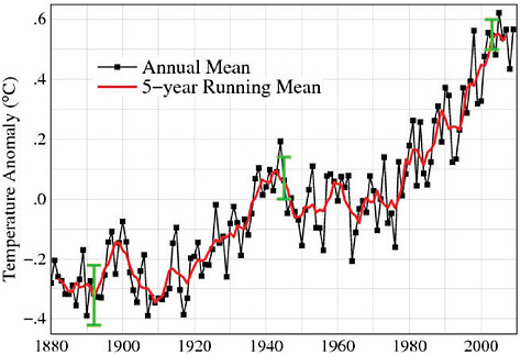
FIGURE 6.12 Global surface temperature (near-surface air temperature over land and sea surface temperatures over ocean areas) change for 1880-2009, reported as anomalies relative to a reference period of 1951-1980, as estimated by NASA GISS (estimates produced by other research teams are very similar). The black curve shows annual average temperatures, the red curve shows a 5-year running average, and the green bars indicate the estimated uncertainty in the data during different periods of the record. SOURCES: NASA GISS (2010; Hansen et al., 2006, updated through 2009; data available at http://data.giss.nasa.gov/gistemp/graphs/).
ward to explain the substantial decadal-scale variability in the surface temperature record, especially the period of relatively flat temperatures from the early 1940s through the late 1970s. Probably the most widely cited hypothesis, which is supported by some statistical analyses and model simulations, is that increasing levels of sulfate aerosols from fossil fuel combustion introduced a cooling effect that offset much of the positive forcing from GHGs during the “flat” part of the record (e.g., Hegerl et al., 2007). This hypothesis seems to be supported by the more pronounced “flattening” in the Northern Hemisphere, relative to the more steady increase in the Southern Hemisphere (where aerosol levels are generally much lower). However, other recent analyses (e.g., Swanson et al., 2009) suggest that natural variations in ocean circulation might also give rise to some of the decadal-scale variations in the global temperature record.
The observed warming is also unevenly distributed around the planet (Figure 6.13). In general, the largest increases in temperature worldwide have occurred over land areas and over the Arctic, which is consistent with the horizontal pattern of warming expected from a positive climate forcing. In the continental United States, on average temperatures rose by 1.5°F (0.81°C) between the first decade of the 20th century and the first decade of the 21st century, or about the same as the global temperature change over this period. There is also a rich tableau of ongoing regional, seasonal, diurnal, and local temperature changes associated with these large-scale, long-term, annual-mean surface warming trends:
-
Recent analyses of temperature trends over the Midwest and northern Great Plains have revealed that winter temperatures in that region have increased by 7°F (4°C) over the past 30 years (USGCRP, 2009a).
-
Late spring and early summer daytime maximum temperatures in the southeastern United States, on the other hand, declined slightly from the 1950s to the mid-1990s (Portmann et al., 2009).
-
An analysis of daily temperature records reveals that during the last decade nearly twice as many extreme record high temperatures have been recorded globally than extreme record low temperatures (Meehl et al., 2009c).
-
Hot days and nights have become warmer and more common, while cold days and nights have become warmer and fewer in number (IPCC, 2007a).
Many of these changes are consistent with the spatial and temporal patterns of temperature change expected to result from increasing GHG concentrations.
|
BOX 6.1 Short-Term Variability Versus Long-Term Trends When conducting scientific analyses, it is important to analyze data in a manner that is consistent with the phenomenon being studied. Climate, for example, is typically defined based on 30-year averages (Burroughs, 2003; Guttman, 1989). This averaging period is chosen, in part, to minimize the influence of natural variability on shorter time scales and facilitate the analysis of long-term trends, especially trends associated with long-term changes in the Earth’s radiative balance. Individual years, or even individual decades, can deviate from the long-term trend due to natural climate variability. Thus, it is not appropriate to look at only a short period of the overall record (such as changes over just the last 5 or 10 years) to infer major changes in the trajectory of global warming. An example of a more familiar temperature trend—one associated with the seasonal cycle—illustrates the importance of analyzing trends over appropriate time scales. The figure below shows daily average temperatures for New York City for the period of January 1 through July 1, 2009. Temperatures would obviously be expected to increase on average over this 6-month period due to the seasonal cycle, but natural variability (which in this case is largely due to the passage of individual weather systems) also gives rise to significant daily, weekly, and even monthly fluctuations in these data. For example, on February 12, 2009, temperatures reached 51°F and then generally declined to 20°F on March 3 (red arrows). Similarly, temperatures reached 78°F on two days in late April before generally declining to 61°F in mid-June (green arrows). It would be incorrect to conclude that summer was not coming based on these two subsets of the data. In a similar manner, one could potentially draw erroneous conclusions about the long-term trend in global surface temperature by focusing exclusively on a subset of the data in the figure—such as data from just the last 10 or 12 years (see also Easterling and Wehner, 2009; Fawcett, 2007; Knight et al., 2009). As discussed in the text, the climate system exhibits substantial year-to-year and even decade-to-decade variability, while global temperature increases due to rising GHG increases, and other radiative forcing factors all operate on longer time scales. Robust analyses of global climate change thus tend to focus on trends over at least several decades.a Scientists often average climate data over several years or decades, or use more sophisticated statistical methods, to make long-term trends more readily apparent. Statistical methods can also be used to identify other important climate patterns and trends, such as changes in extreme events or shifts in modes of natural variability. |
Atmospheric Temperatures
In addition to surface-based thermometer measurements, regular and widespread measurements of the vertical profile of atmospheric temperatures are available from both satellites and weather balloons for the last several decades. Weather balloons, which are launched twice per day from over 800 sites around the world, carry instruments known as radiosondes that directly measure atmospheric conditions and radio these data back to receiving stations. Although these measurements are taken primar-
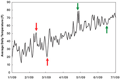 New York City daily average temperature for the first 6 months of 2009. Red and green arrows denote the beginning and end of two periods when temperatures declined on average, despite an overall warming trend due to the seasonal cycle. SOURCE: NCDC (2006).
|
ily to support weather prediction, researchers have developed methods for aggregating the data, removing a variety of systematic biases (including changes in instrumentation, the fact that all of the balloons are launched at the same two times each day, which means they are launched at different local times, and a recently identified bias associated with the sun heating the instruments) to yield a record of three-dimensional changes in atmospheric temperature over the last 50 years (McCarthy et al., 2008).
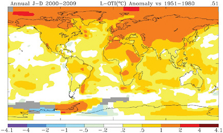
FIGURE 6.13 Average surface temperature trends (degrees per decade) for the decade 2000-2009 relative to the 1950-1979 average. Warming was more pronounced at high latitudes, especially in the Northern Hemisphere, and over land areas. SOURCES: NASA GISS (2010; Hansen et al., 2006, with 2009 update).
Regular satellite-based observations of temperature and other atmospheric properties began in the late 1970s. Rather than directly sampling atmospheric conditions, satellites measure the upwelling radiation from the Earth at specific wavelengths, and this information can be used to infer the average temperature of different layers in the atmosphere underneath. As with surface temperature records, the raw satellite data are analyzed by several different research teams, each using its own techniques and assumptions, to produce estimates of inferred temperature changes (Christy et al., 2000, 2003; Mears and Wentz, 2005). While satellite-derived data offer the advantage of excellent global coverage, they still require corrections to remove artificial biases, such as the slow decay of satellite orbits and changes in instrumentation when satellites are replaced. The fact that satellite-inferred temperatures represent layers of the atmosphere rather than specific points in space also leads to some uncertainties in the analysis and interpretation of the data—for example, it was recently demonstrated that previous estimates of lower-atmosphere warming from satellites were biased slightly downward due to the inclusion of some data from the stratosphere, which has cooled (see next paragraph; also Fu et al., 2004). As discussed in Chapter 4 and in some of the other chapters in Part II, satellite data also offer a wealth of information about other changes in the Earth system.
Radiosonde and satellite-derived data both show that the troposphere (the lowest layer of the atmosphere, extending up to roughly 10 miles [16 km] in the tropics and 6 miles [10 km] near the poles) has warmed substantially over the past several decades (Figure 6.14). The most recent analyses of satellite data from 1979 through the end of 2009 estimate a tropospheric warming of +0.23°F (+0.13°C) per decade (Christy et al., 2000, 2003) to +0.28°F (+0.15°C) per decade (Mears and Wentz, 2005; RSS, 2009), while radiosonde-derived temperature estimates yield +0.30°F (+0.17°C) per decade for the same time period and +0.29°F (+0.16°C) for the full radiosonde record starting in 1948 (HadAT2; McCarthy et al., 2008). For comparison, surface temperatures increased +0.29°F (+0.16°C) per decade since 1979 and +0.23°F (0.13°C) per decade since 1948.
Additionally, radiosondes and satellites both indicate that the stratosphere has cooled even more strongly than the troposphere has warmed (Figure 6.14, top panel). This
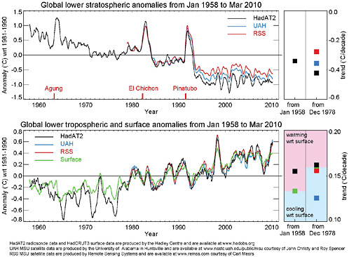
FIGURE 6.14 Radiosonde- (black) and satellite-based (blue and red) estimates of temperature anomalies for 1958-2009 in the (top) stratosphere and (bottom) troposphere. The squares on the right-hand side of the figure indicate the trends in each data series from two different start dates. SOURCE: Hadley Center (data available at http://hadobs.metoffice.com/hadat/images.html).
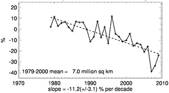
FIGURE 6.15 Satellite-based trend of September (end of summer) Arctic sea ice extent for the period 1979 to 2009, expressed as percentage difference from 1979-2000 average sea ice extent (which was 7.0 million square miles). These data show substantial year-to-year variability, but a long-term decline in sea ice extent is clearly evident, as highlighted by the dashed linear trend line. As discussed in the text, the average thickness of Arctic sea ice has also declined markedly over the last 50 years. SOURCE: NSIDC (2010).
vertical pattern of temperature change, with warming in the troposphere and cooling in the upper atmosphere, is consistent with the pattern expected due to increasing GHG concentrations (Roble and Dickinson, 1989). Current research on temperature trends focuses on, among other issues, regional, seasonal, and day-night differences in temperature trends, especially in the tropics, where climate models predict a stronger warming in the upper troposphere than has been observed to date (e.g., Fu and Johanson, 2005).
Other Indicators of Climate Change
Additional direct indicators of a warming trend over the last several decades can be found in the cryosphere and oceans. As discussed in detail in Chapter 7, the vast majority of the total heating associated with human-caused GHG emissions has actually gone into the world’s oceans, which have warmed substantially over the last several decades (Levitus et al., 2009). In the cryosphere, mountain glaciers and ice-caps are melting (these changes are also discussed in detail in Chapter 7), rivers and lakes are thawing earlier and freezing later in the year (Rosenzweig et al., 2007), and winter snow cover (Trenberth et al., 2007) and summer sea ice (Figure 6.15) are both decreasing in the Northern Hemisphere. Analyses of recently declassified data from naval submarines (as well as more recent data from satellites) show that the aver-
age thickness of sea ice in the Arctic Ocean has declined substantially over the past half-century, which is yet another indicator of a long-term warming trend (Kwok and Rothrock, 2009). Warming can also be inferred from a host of ecosystem changes: flowers are blooming earlier, bird migration and nesting dates are shifting, and the ranges of many insect and plant species are expanding poleward and to higher elevations—these and other trends in biological systems are discussed in detail in Chapter 9.
Scientists have collected a wide array of indirect evidence of how temperature and other climate properties varied before instrumental measurements became available. These so-called “proxy” climate data are derived from a diverse range of sources including ice cores, tree rings, corals, lake sediments, records of glacier length, bore-hole temperature measurements, and even historical documents. A recent assessment of these data and the techniques used to analyze them (NRC, 2006b) concluded that, although proxy data generally become scarcer, less consistent, and more uncertain going back in time, temperatures during the past few decades were warmer than during any other comparable period for at least the last 400 years, and possibly for the last 1,000 years or longer (Figure 6.16). Proxy-based temperature and forcing estimates for the past millennium, and for longer time periods such as the Ice Age cycles described above, illustrate the natural variability of the climate system on a wide range of time scales. These estimates are also used to help constrain estimates of climate sensitivity.
While temperature and temperature-related changes are the most widely cited and typically the best-understood changes in the physical climate system, a host of concomitant and related changes have also been observed. For example, the absorption of CO2 by the oceans is causing widespread ocean acidification, with significant implications for natural ecosystems and fisheries (as discussed in Chapters 9 and 10, respectively). There have also been significant changes in the overall amount, patterns, and timing of precipitation both globally and in the United States, and the characteristics of these precipitation changes are consistent with what would be expected for GHG-induced warming (see Chapter 9). A number of changes in atmospheric circulation patterns have also been observed (e.g., Fu et al., 2006).
Finally, it should be noted that the observed changes in the climate system to date represent only a fraction of the total expected changes associated with the GHGs currently in the atmosphere: Even if the current climate forcing were to persist indefinitely, it is estimated that the Earth would warm another 0.6°C (1.1°F) over the next several decades as the oceans slowly warm in response to the current GHG forcing, with concomitant changes in other parts of the Earth system (this so-called “commitment warming” is discussed in further detail below). In addition, since CO2 and many other GHGs remain in the atmosphere for hundreds or even thousands of years
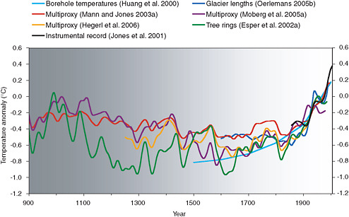
FIGURE 6.16 Estimates of surface temperature variations for the last 1,100 years derived from different combinations of proxy evidence (colored lines). Each curve portrays a somewhat different history of temperature variations and is subject to a somewhat different set of uncertainties that generally increase going backward in time (as indicated by the gray shading), but collectively these data indicate that the past few decades were warmer than any comparable period for at least the last 400 years, and possibly for the last 1,000 years. SOURCE: NRC (2006b).
(Solomon et al., 2009), an additional 2.5°F (1.4°C) of global warming is possible over the next several centuries due to ice sheet disintegration, vegetation change, and other long-term feedbacks in the climate system (Hansen et al., 2008). However, these processes are generally less well understood than the feedbacks that give rise to climate change on shorter (e.g., decadal) time scales.
Attribution of Observed Climate Change to Human Activities
Many lines of evidence support the conclusion that most of the observed warming over at least the last several decades is due to human activities:
-
Both the basic physics of the greenhouse effect and more detailed calculations using sophisticated models of atmospheric radiative transfer indicate
-
that increases in atmospheric GHGs should lead to warming of the Earth’s surface and lower atmosphere (NRC, 2005d).
-
Earth’s surface temperature has unequivocally risen over the past 100 years, to levels not seen in at least several hundred years and possibly much longer (NRC 2006b), at the same time that human activities have resulted in sharp increases in CO2 and other GHGs (as discussed above).
-
Detailed observations of temperatures, GHG increases, and other climate forcing factors from an array of instruments, including Earth-orbiting satellites, reveal an unambiguous correspondence between human-induced GHG increases and planetary warming over at least the past three decades, in addition to substantial year-to-year natural climate variability (Hegerl et al., 2007).
-
The vertical pattern of atmospheric temperature change over the past few decades, with warming in the lower atmosphere and cooling in the stratosphere (see Figure 6.15), is consistent with the pattern expected due to GHG increases and inconsistent with the pattern expected if other climate forcing agents (e.g., changes in solar activity) were responsible (Roble and Dickinson, 1989).
-
Estimates of changes in temperature and forcing factors over the first seven decades of the 20th century are slightly more uncertain and also reveal significant decadal-scale variability (see Figure 6.12), but nonetheless indicate a consistent relationship between long-term temperature trends and estimated forcing by human activities.
-
The horizontal pattern of observed surface temperature change over the past century, with stronger warming over land areas and at higher latitudes (Figure 6.13), is consistent with the pattern of change expected from a persistent positive climate forcing (see, e.g., Schneider and Held, 2001).
-
Detailed numerical model simulations of the climate system (see the following section for a discussion of climate models) are able to reproduce the observed spatial and temporal pattern of warming when anthropogenic GHG emissions and aerosols are included in the simulation, but not when only natural climate forcing factors are included (Randall et al., 2007).
-
Both climate model simulations and reconstructions of temperature variations over the past several centuries indicate that the current warming trend cannot be attributed to natural variability in the climate system (Jansen et al., 2007; NRC, 2006b).
-
As discussed earlier in this chapter, estimates of climate forcing and temperature changes on a range of time scales, from the several years following volcanic eruptions to the 100,000+ year Ice Age cycles, yield estimates of climate
-
sensitivity that are consistent with the observed magnitudes of observed climate change and estimated climate forcing.
-
Finally, there is not any compelling evidence for other possible explanations of the observed warming, such as changes in solar activity (Lean and Woods, in press), changes in cosmic ray flux (Benestad, 2005), natural climate variability (Hegerl et al., 2007), or release of heat stored in the deep ocean or other climate system components (Barnett et al., 2005a).
FUTURE CLIMATE CHANGE
Climate Forcing Scenarios
In order to project future changes in the climate system, scientists must first estimate how GHG emissions and other climate forcings will evolve over time. Since the future cannot be known with certainty, a large number of scenarios of future emissions are developed using different assumptions about future economic, social, technological, and environmental conditions. Emissions scenarios are not forecasts and do not attempt to predict “short-term” fluctuations such as business cycles or oil market price spikes. Instead, they focus on long-term (e.g., decades to centuries) trends in energy and land use that ultimately affect the radiation balance of the Earth.
For the past decade, the most widely used scenarios of 21st-century GHG emissions have been those produced for the IPCC’s Special Report on Emissions Scenarios (SRES) (Nakicenovic, 2000). The SRES scenarios are quantitative realizations of qualitative storylines that sketched a range of alternative assumptions regarding 21st-century population growth and economic and technological development. The SRES scenarios were all intended to represent alternative baseline (or “business as usual”) GHG emissions trajectories, with no explicit policy interventions to limit emissions. In addition, probability distributions were not estimated for either the range or individual SRES scenarios, and so there was no explicit characterization of the likelihood that actual emissions might fall outside the range of the included scenarios.
Since 2000, major scenario exercises have put less emphasis on alternative no-policy baselines and instead concentrated primarily on elaborating the socioeconomic, technological, and policy aspects of alternative GHG trajectories over the next century, with an emphasis on changes over the next few decades; on improving the realism and comprehensiveness of both individual scenarios and the suite of scenarios, for example by adding or improving representations of all important forcing agents and developing scenarios with widely spaced total radiative forcing estimates; and on developing these trajectories in a more integrated and iterative manner with climate model
projections and assessments of current and future climate impacts. Recent scenario development exercises stressing these characteristics have been undertaken by the CCSP (2007c), the Energy Modeling Forum (Clarke et al., 2009), and other groups (Moss et al., 2010). These exercises have yielded a number of important insights, such as the challenges associated with reaching certain GHG emissions or temperature goals.
The aim of developing more useful climate forcing scenarios is subject to several pressures that are in tension with each other, such as providing more sophisticated and increasingly detailed representations of socioeconomic, environmental, and policy factors, while at the same time keeping the origin of the assumptions used transparent, plausible, and understandable. Additional challenges to scenario development include balancing and integrating the qualitative and quantitative elements of scenarios; developing scenarios that provide socioeconomic and environmental information (which is useful, for example, for adaptation planning) that is consistent with the corresponding emissions trajectories; and making more explicit, transparent, and defensible judgments of probabilities associated with scenario-based ranges of key variables (CCSP, 2007b; Parson, 2008).
In response to these issues, climate modelers, integrated assessment modelers, and researchers focusing on impacts, adaptation, and vulnerability collaborated to develop a new process for preparing and applying scenarios in climate research (Moss et al., 2010). In contrast to the traditional approach in which scenarios are developed and applied in a linear causal chain from socioeconomic “drivers” of emissions, to atmospheric and climate processes, to impacts, the new process starts with four scenarios of future radiative forcing called “Representative Concentration Pathways.” These pathways are defined by their radiative forcing in 2100 and include (1) a high scenario of 8.5 W/m2, and still rising; (2) an “overshoot scenario” in which radiative forcing peaks midcentury and then declines to a level of 2.6 W/m2 (which is lower than any of the SRES scenarios) in 2100, and (3) two intermediate scenarios that stabilize in 2100 at 6 and 4.5 W/m2. These representative concentration pathways will be used to conduct new climate model experiments and produce new climate change scenarios. In parallel, new socioeconomic and emissions scenarios will be developed to explore detailed scenarios of socioeconomic drivers, adaptation, mitigation, and other issues such as feedbacks. The process rests on the simple observation that any particular radiative forcing trajectory can be realized by many different socioeconomic, technology, and policy futures. The new process facilitates research into a number of key issues including feedbacks, the ease or difficulty of achieving overshoot scenarios (and the climate and ecosystem consequences of these trajectories, which are highly uncertain), as well as process issues discussed in the previous paragraph.
Climate Models
Climate models encapsulate scientists’ best understanding of climate and related Earth system processes and are important tools for understanding past, present, and future climate change. While there are many different kinds of climate models, all are based fundamentally on the laws of physics that govern atmospheric and oceanic motions, including the conservation of mass, energy, and angular momentum and laws that govern the propagation of radiation through the atmosphere. Most modern climate models also include representations of the oceans, cryosphere, and land surface, as well as the exchanges of energy, moisture, and materials among these components. Earth system models additionally simulate a wide range of biophysical processes including atmospheric chemistry and the biogeochemistry of ecosystems on land and in the oceans (Figure 6.17).
Climate and Earth system models (for simplicity, referred to hereafter as climate models) use computer-based numerical techniques to solve a system of mathematical equations that embody these laws, systems, and processes, yielding a predicted evolution of the climate system over time (see, e.g., DOE, 2008b, 2009b; Donner and
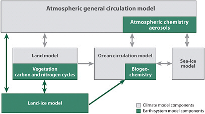
FIGURE 6.17 Schematic illustration of the components of climate and Earth system models. The components of climate models are in gray and the additional components in Earth system models are in green. The connecting arrows indicate exchanges that couple the model components. SOURCE: Donner and Large (2008).
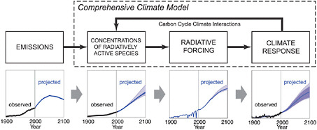
FIGURE 6.18 Schematic overview of the translation from a specified trajectory of emissions of GHGs and other climate forcing agents to trajectory to climate response. Simulated climate changes will include both the forced response and internal (natural) variability. The specific model results in the bottom row are for illustrative purposes only. SOURCE: Meehl et al. (2007a).
Large, 2008). Climate models are based on the same basic equations that are used to predict short-term weather variations. However, rather than trying to predict the exact future evolution of the atmosphere (i.e., the weather), climate models instead focus on accurately simulating the processes that govern interannual and longer-term climate trends (see Box 6.1).
Climate models are used to simulate both natural climate variability and the evolution of the climate system under specified climate forcing, including both historical data and scenarios of future forcing changes (Figure 6.18). Our confidence in the ability of climate models to reliably project certain aspects of future climate stems from the extensive development and testing processes used to design models and evaluate their performance—including simulations of 20th-century climate when the climate forcing and response are both reasonably well known (up to the limits of observations and recordkeeping) and simulations of the response to volcanic eruptions (e.g., Randall et al., 2007). Moreover, by assessing many different models, each with different emphases, strengths, and weaknesses, or many different runs of the same model (which provides an indication of natural variability), the most robust features of future projections emerge. These results are presented in the next section of the chapter.
Advances in climate modeling over the past 50 years have been driven by two main factors: (1) increases in computer power, which have allowed improved spatial resolution, the inclusion of additional Earth system components, more explicit representa-
tions of processes, and multiple model experiments to explore different assumptions and model specifications; and (2) improvements in theoretical and mechanistic understanding of the climate system and the processes being modeled, which in turn are tied to basic research and improvements in observational capabilities. Today, continued improvements in computational power, scientific understanding, and supporting observations are still the primary factors driving improvements in climate models—or stated conversely, even if the evolution of future climate forcing were known exactly, limits in computer power, observational data, and scientific understanding of the climate system would still constrain the ability of models to produce perfect predictions of future climate (Shapiro et al., in press).
For example, the typical horizontal grid spacing of a state-of-the-art global climate model is on the order of 60 miles (100 km), but climatically relevant features such as clouds, topography, and land cover often vary at a scales of a half-mile or less. These subgridscale features and processes must be parameterized—approximated using numerical techniques that specify the large-scale influence of small-scale processes—or upscaled through statistical or “nested model” approaches that extend representative small-scale simulations to larger spatial scales. As a result of these approximations and other factors (described below), global climate models generally only provide consistent and reliable simulations of temperature, precipitation, and other relevant climate variables at continental to global scales.
Regional Climate Projections
The lack of regionally specific climate information from global climate models poses a major challenge, because many climate-related decisions, especially those related to adaptation, demand information on regional to local scales. A variety of downscaling approaches have been developed to obtain this regional information. One widely used approach is statistical downscaling, wherein empirical relationships between past observations of local- and regional-scale climate variations are used to translate large-scale projections from global climate models to smaller space scales and shorter time scales. Alternatively, finer-scale regional models can be “nested” within coarser-resolution global models to simulate regional climate changes (e.g., Hay et al., 2002; Leung et al., 2003; UCAR, 2007). A related approach is linking models currently used to predict weather and seasonal to interannual climate variations with those that predict climate change on decadal to centennial time scales (this is sometimes called “seamless prediction”).
In general, downscaling techniques are not as well developed or understood as global
models, and key technical and scientific issues remain. For example, regional modeling efforts have been limited by constraints on computing resources, uncertainties and complexities associated with data assimilation and parameterization, the lack of a well-developed framework for downscaling, and the limitations of the large-scale simulations on which the downscaling is performed (Held and Soden, 2006; NRC, 2009k). An additional challenge for regional projections is representing regional modes of variability, such as ENSO and the Pacific Decadal Oscillation (described earlier in this chapter). Not only do these regional modes have a strong influence on local and regional climate change, but many also have global signatures, and they could potentially change themselves as the climate system warms. Finally, climate forcing scenarios that project human influences on local and regional climate, such as regional aerosol loading and land use change, are needed because these forcings may have a large influence on local and regional climate change (CCSP, 2008c).
Projections of 21st-Century Climate
The most comprehensive suite of climate modeling experiments performed to date were completed in 2005 as part of the World Climate Research Programme’s Coupled Model Intercomparison Project phase 3 (CMIP3; Meehl et al., 2007b) in support of the IPCC’s Fourth Assessment Report. CMIP3 included 23 different state-of-the-art models from groups around the world, all of which were run with a specific set of emissions scenarios (based on the SRES report described above) to facilitate comparison and synthesis of results. As described in detail by the IPCC (Meehl et al., 2007a), the CMIP3 climate models project increases in mean surface temperatures over the 21st century ranging from 2.0°F to 11.5°F (1.1°C to 6.4°C), relative to the 1980-1999 average, by the end of the century.
Figure 6.19 shows projected global temperature changes associated with three representative scenarios of high, medium-high, and low future GHG emissions. The separation between the three curves illustrates the uncertainty associated with the choice of scenario, while the uncertainties associated with differences among different models in simulating the climate system can be inferred from the shading surrounding each curve. The “commitment warming” associated with emissions through the year 2000 and, for two of the future forcing scenarios, through 2100 are also shown. These “commitment” runs, which are performed by instantaneously stabilizing atmospheric GHG concentrations, show that the climate system will continue to warm for several centuries after GHG emissions are stabilized—illustrating the inherent time lag between GHG emissions and the long-term climate response.
As with observed climate change to date, regional manifestations of future climate projections vary substantially, with stronger warming over higher latitudes and land areas (Figure 6.20). The similarity between the three panels on the left-hand side of Figure 6.20 also illustrates how temperature increases over the next few decades reflect past emissions as well as somewhat similar GHG emissions over the next few decades for the three selected SRES scenarios (none of which include explicit policy interventions). By midcentury and especially at the end of the century, however, the medium- and high-emissions scenarios clearly lead to much warmer temperatures than the lower-emissions scenario. U.S. temperatures are projected to warm substantially over the 21st century under all emissions scenarios (USGCRP, 2009a).
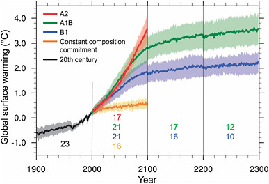
FIGURE 6.19 Model simulations of changes in global average temperature from 1900 to 2300. The black line and gray shading shows the average and spread1 of 23 model simulations of 20th-century climate using estimates of actual climate forcing. The colored lines and shading show average and spreads for projected global average temperatures for the 21st century under four different scenarios of future forcing: a “high-emissions” scenario (red), a “medium-high” scenario (green), a “low-emissions” scenario (blue), and a “commitment” scenario (orange), which assumes that GHG concentrations remain constant at year 2000 values. The green and blue curves also show commitment experiments for the 22nd and 23rd centuries (i.e., with the forcing at year 2100 held constant thereafter). Changes are relative to the 1960-1979 average. See text for additional discussion. SOURCE: Meehl et al. (2007a).
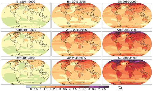
FIGURE 6.20 Worldwide projected changes in temperatures, relative to 1961-1990 averages, under three different emissions scenarios (rows) for three different time periods (columns). Projected warming is much stronger over land areas and high latitudes. SOURCE: Meehl et al. (2007a).
In addition to average temperature, a host of other climate variables are projected to experience significant changes over the 21st century, just as they have during the past century. For example, the frequency and intensity of heat waves is projected to continue to increase, both in the United States (Figure 6.21) and around the world. This projection is considered robust because a shift in the average value of a temperature distribution (or in another climate variable) typically entails an increase in the frequency of extreme and unprecedented events (see, e.g., Solomon et al., 2007). Similarly, there is considerable confidence that the frequency of cold extremes will decrease and that the number of frost days will decline in the middle and high latitudes, following current trends (Meehl et al., 2007a; USGCRP, 2009a). Projections of future climate also indicate that snow cover and sea ice extent will continue to decrease (Meehl et al., 2007a; USGCRP, 2009a; Zhang, 2010), while sea level will continue to rise (see Chapter 7).
Projections of precipitation change are generally more uncertain than projections of temperature and temperature-related changes. However, most models project increased precipitation in northern regions of the United States, while it is considered very likely that the southwestern United States will experience a net decrease in precipitation (USGCRP, 2009a). Another robust projection, which results from the fact
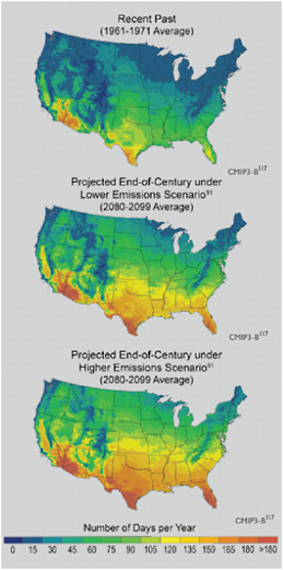
FIGURE 6.21 Projected changes in number of very hot days in the United States for lower- and higher-emissions scenario. The number of very hot days will increase substantially across virtually the entire country, in some places doubling or even trebling the number of days above 90°F. SOURCE: USGCRP (2009a).
that warmer air can hold more moisture, is that the fraction of rainfall falling in the form of heavy precipitation events will increase in many regions (Meehl et al., 2007a). These and other projected changes in precipitation, and the impact of these changes on freshwater resources, are explored in Chapter 8. Later chapters also explore how changes in temperature, precipitation, and other aspects of the physical climate system are likely to affect ecosystems (see Chapter 9), agriculture (Chapter 10), human health (Chapter 11), the urban environment (Chapter 12), transportation (Chapter 13) and energy systems (Chapter 14), and national security (Chapter 16).
Key Uncertainties in Projections of Future Climate
A great deal is known about past, present, and projected future climate change, especially at large (continental to global) scales. For example, there is high confidence that global temperatures will continue to rise, that the rate and magnitude of future temperature change depends strongly on current and future rates of GHG emissions, and that climate change—in interaction with other global and regional environmental changes—poses significant risks for a number of human and natural systems. Global climate models and, increasingly, regional techniques are also starting to provide useful information about future climate and climate-related changes on local to regional scales. Some of these projections—such as increases in extreme heat events and Arctic sea ice—are quite robust, while others are somewhat more speculative.
There are, however, several aspects of future climate change that remain more uncertain, and these represent some of the most important and active areas of current scientific research (see Research Needs at the end of this chapter). The uncertainties in climate projections can be categorized into two main sources: (1) uncertainties in future climate forcing and (2) uncertainties in how the climate system will respond to forcing, which includes both the known limitations of global climate models (such as an inability to resolve individual clouds) and the fact that the climate system is complex and might exhibit novel or unanticipated behavior in response to ongoing climate change.
The first of these categories, uncertainties in future climate forcing, was discussed in the Future Climate Scenarios section earlier in the chapter. The spread among the three colored curves in Figure 6.20 provides a rough indication of the importance of this uncertainty in terms of the magnitude of future climate change. As discussed above, and described in further detail in the companion report Limiting the Magnitude of Future Climate Change (NRC, 2010c), future climate forcing depends strongly on the choices that current and future human societies make, especially regarding energy production and use. However, actions that might be taken to limit the magnitude of future climate change, or adapt to its impacts, have not yet been fully and systematically integrated into climate forcing scenarios and evaluated across a range of different climate models to determine how they might ultimately affect both climate and other aspects of the Earth system.
As an illustration of some of the uncertainties present in climate model projections, Figure 6.22 shows projections of temperature change over North America from 21 different models, each using the same scenario of future climate forcing. Several robust features emerge from these projections—for example, all of the models project a
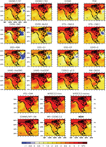
FIGURE 6.22 Projected warming for the 21st century (difference between 2080-2099 temperature and 1980-1999 temperature) for the North American region using 21 different climate models, all using the same scenario of future GHG emissions. The mean (average) of the 21 model experiments is also shown in the bottom right panel. Several robust features are evident, including enhanced warming over land areas and higher latitudes. Differences among the 21 projections are indicative of some of the uncertainties associated with model projections. SOURCE: Christensen et al. (2007).
substantial overall temperature increase, with stronger warming over land areas and at higher latitudes. Most of the models show somewhat less warming over the southeastern United States and a slight cooling, or at least less warming, over the western North Atlantic Ocean south of Greenland. In other regions, however, the exact pattern and magnitude of projected warming varies considerably among models. Typically, the average of many climate model simulations represents a more robust projection than any individual projection (Randall et al., 2007), so the average of these model calculations (shown in the bottom right panel) can be thought of as the most reliable prediction of future temperature change over North America. Differences among models indicate some (but not all) of the uncertainty in this “multimodel mean” projection. Analyses of the differences among models—such as CMIP3 and previous model intercomparison projects—are also a key tool for model development.
The other main type of “known” uncertainty in model-based projections of future climate change is associated with processes that are either not resolved or not very well simulated in the current generation of global climate models. These processes, which are discussed in further detail in the Research Needs section at the end of this chapter, include clouds and aerosols, the carbon cycle, ocean mixing processes, ice sheet dynamics, ecosystem processes, land use–related changes, and extreme weather events such as hurricanes, tornadoes, and droughts. Another key research area is the relationship between regional modes of variability and global climate change, including the possibility that regional variability modes may shift in response to either regional or global human activities.
Abrupt Changes and Other Climate Surprises
Confounding all projections of future climate is the possibility that abrupt changes or other climate “surprises” may occur. Abrupt changes in the climate system can occur when (1) there is a rapid change in forcing, such as a rapid increase in atmospheric GHG concentrations or reduction in aerosol forcing, or (2) thresholds for stability (or “tipping points”) are crossed, such that small changes in the climate state are reinforced, leading to rapid shifts until the climate enters another stable state and stability is restored. Paleoclimate records indicate that the climate can go through abrupt changes in as little as a single decade (NRC, 2002a). For example, Greenland ice cores indicate that about 13,000 years ago, during the recovery from the last Ice Age, local temperatures fell more than 10°F (6°C) within a few decades and remained low for more than a millennium before jumping up more than 16°F (10°C) in about a decade (CCSP, 2007b). Since the Earth’s temperature is now demonstrably higher than it has been for at least 400 years and possibly more than 1,000 years (NRC, 2006b), and GHG
concentrations are now higher than they have been in many hundreds of thousands of years, it is possible that we may be nearing other stability thresholds. However, we have only a limited understanding of what those thresholds might be or when the climate system might be approaching them.
One example of a potential abrupt change mechanism is the possibility that GHGs stored in permafrost (frozen soils) across the Arctic could be released in large quantities as high-latitude warming continues. Permafrost contains huge amounts of carbon that have been locked away from the active carbon cycle for millennia, and it has been demonstrated that thawing permafrost releases some of this carbon to the atmosphere in the form of CH4 and CO2 (Shakova et al., 2010). If the release of these GHGs accelerates as the Arctic continues to warm, this could potentially accelerate the warming, leading to a positive feedback on the warming associated with GHGs released through human activities (Lawrence and Slater, 2005; Schuur et al., 2009; Zimov et al., 2006). In a related example, high-latitude warming can also alter the types of ecosystems covering the land (for instance, a shift from tundra to forest), which in turn changes the reflective characteristics of the land surface and thus potentially exerts a further positive feedback on warming (Field et al., 2007a).
Other potential abrupt changes include rapid disintegration of the major ice sheets (see Chapter 7), irreversible drying and desertification in the subtropics as a result of shifts in circulation patterns (see Chapter 8), changes in the meridional overturning circulation in the ocean (Broecker, 1997, 2002; Stocker, 2000; Stocker and Schmittner, 1997), or the rapid release of CH4 from destabilized methane hydrates in the oceans (Archer and Buffet, 2005; Overpeck and Cole, 2006), all of which could dramatically alter the rate of both regional and global climate change. Other surprises that may be associated with future climate change include so-called “low-probability, high-impact” events, such as an unprecedented heat wave or drought, or when multiple climate changes interact with each other or with other environmental stresses to yield an unexpectedly severe impact on a human or environmental system. Some of these potential—or in some cases already observed—surprises are discussed in later chapters.
RESEARCH NEEDS
Advances in our understanding of the climate system have been and will continue to be a critical underpinning for evaluating the risks and opportunities posed by climate change as well as evaluating and improving the effectiveness of different actions taken to respond. Hence, even as actions are taken to limit the magnitude of future climate change and adapt to its impacts, it is important that continued progress be
made in observing all aspects of the climate system, in understanding climate system processes, and in projecting the future evolution of the climate system, and as well as its interactions with other environmental and human systems (which are explored in the chapters that follow). The following are some of the most critical basic research needs in these areas.
Expand and maintain comprehensive and sustained climate observations to provide real-time information about climate change. Regular and sustained observations of climate variables are needed to monitor the progress of climate change, inform climate-related decision making, and to monitor the effectiveness of actions taken to respond to climate change. Observations are also critical for developing and testing climate models, projections of future climate forcing, and other tools for understanding and projecting climate change, as well as for supporting decision-support activities. As discussed in Chapter 3, a comprehensive climate observing system is needed to provide regular monitoring of biological, chemical, geological, and physical properties in the atmosphere, oceans, land, and cryosphere, as well as related biological, ecological, and socioeconomic processes. Expanded historical and paleoclimatic records would also be valuable for understanding natural climate variations on all time scales and how these modes of variability interact with global climate change. Finally, a comprehensive data assimilation system is also needed to bring these disparate observations into a common framework, so that the state of the whole Earth system can be assessed and impending feedbacks that could alter the rate of climate change can be identified. Research is especially needed on how to better integrate physical indicators with emerging indicators of ecosystem health and human well-being, as discussed in other chapters.
Continue to improve understanding of climate variability and its relationship to climate change. Great strides have been made in improving our understanding of the natural variability in the climate system over the past several decades. These improvements have translated directly into advances in detecting and attributing human-induced climate change, simulating past and future climate in models, and understanding the links between the climate system and other environmental and human systems. For example, the ability to realistically simulate natural climate variations, such as the El Niño-Southern Oscillation, is a critical test for climate models. Improved understanding of regional variability modes is also critical for improving regional climate projections, as discussed below. Understanding the impacts associated with natural climate variations also provides insight into the possible impacts of human-induced climate change. Continued research on the mechanisms and manifestations of natural climate variability in the atmosphere and oceans on a wide range of space and
time scales, including events in the distant past, can be expected to yield additional progress.
Develop more informative and comprehensive scenarios of drivers of future climate forcing and socioeconomic vulnerability and adaptive capacity. Uncertainty in projections of the future is inevitable. However, the development of scenarios allows better understanding of the dynamics of the interconnected human-environment system and in particular how the dynamics will change depending on the choices we make. Scenarios are also critical for helping decision makers establish targets for future GHG emissions and concentration levels as well as helping make plans to adapt to the future projected impacts of climate change, topics addressed in many of the chapters that follow. Developing and improving assessments of the potential influence of various policy choices on emission profiles and adaptive capacity is particularly important in the context of supporting climate-related decision making—especially “overshoot” scenarios, which have the potential to cause irreversible changes to the climate system. Influences of shorter-lived forcing agents (including short-lived GHGs and aerosols) are also of high importance in the near term and could benefit from more near-term emphasis.
Developing enhanced scenarios and linking them to a variety of Earth system and socioeconomic models is an inherently interdisciplinary and integrative activity requiring contributions from many different scientific fields as well as processes that link scientific analysis with decision making and, ideally, public deliberation about desirable futures. The new “Representative Concentration Pathways” described earlier represent a few common, transparent, thoroughly documented representative scenarios of key variables over time. A number of research needs and developments are required to develop new socioeconomic scenarios that explore both mitigation and adaptation issues. It is particularly important to explore methods for coupling scenarios across geographic scales (from global to regional to local), to further develop methods for downscaling climate scenarios and providing regional climate information, and to develop data and information systems for pairing socioeconomic and climate scenarios for use in impacts research and to support the needs of particular decision makers.
Improve understanding of climate system forcing, feedbacks, and sensitivity. The past several decades have seen tremendous progress in quantifying human influences on climate and assessing the response of the climate system to these influences. This progress has been critical both in establishing the current level of confidence in human-induced climate change and in developing reliable projections of future changes. Key uncertainties remain, however, and continued research on the basic mechanisms
and processes of climate change can be expected to yield additional progress. Some critical areas for further study include the following:
-
Continued research to improve estimates of climate sensitivity, including theoretical, modeling, and observationally based approaches;
-
Improved understanding of cloud processes, aerosols and other short-lived forcing agents, and their interactions, especially in the context of radiative forcing, climate feedbacks, and precipitation processes;
-
Continued theoretical and experimental research on carbon cycle processes in the context of climate change, especially as they relate to strategies for limiting climate change (CCSP, 2007a; NRC, 2010j);
-
Improve understanding of the relationship between climate change and other biogeochemical changes, especially acidification of the ocean (see Chapter 9);
-
Improve understanding of the hydrologic cycle, especially changes in precipitation (see also Chapter 8);
-
Improved understanding of the mechanisms, causes, and dynamics of changes in the cryosphere, especially changes in major ice sheets (see Chapter 7) and sea ice.
Overall, the need for improved understanding of climate forcing, feedbacks, and sensitivity was summarized well in the NRC report Understanding Climate Change Feedbacks (NRC, 2003b); these suggestions remain highly relevant today:
The physical and chemical processing of aerosols and trace gases in the atmosphere, the dependence of these processes on climate, and the influence of climate-chemical interactions on the optical properties of aerosols must be elucidated. A more complete understanding of the emissions, atmospheric burden, final sinks, and interactions of carbonaceous and other aerosols with clouds and the hydrologic cycle needs to be developed. Intensive regional measurement campaigns (ground-based, airborne, satellite) should be conducted that are designed from the start with guidance from global aerosol models so that the improved knowledge of the processes can be directly applied in the predictive models that are used to assess future climate change scenarios.
The key processes that control the abundance of tropospheric ozone and its interactions with climate change also need to be better understood, including but not limited to stratospheric influx; natural and anthropogenic emissions of precursor species such as NOx, CO, and volatile organic carbon; the net export of ozone produced in biomass burning and urban plumes; the loss of ozone at the surface, and the dependence of all these processes on climate change. The
chemical feedbacks that can lead to changes in the atmospheric lifetime of methane also need to be identified and quantified.
Improve model projections of future climate change. Numerous decisions about climate change, including setting emissions targets and developing and implementing adaptation plans, require information that is underpinned by models of the physical climate system. There are a number of scientific and technological advances needed to improve model projections of future changes in the Earth system, especially changes over the next several decades and at the local and regional levels where many climate-related decisions occur. While this research should not be expected to eliminate uncertainties, especially given the inherent uncertainty in projections of future climate forcing, efforts to expand and improve model simulations of future climate changes can be expected to yield more, more robust, and more relevant information for decision making, including the effectiveness of various actions that can be taken to respond to climate change. It should also be noted that improvements in modeling go hand-in-hand with improvements in understanding and observation.
The core of the nation’s climate modeling enterprise is the development and testing of global Earth system models, many of which already or are now beginning to incorporate some of the key forcing and feedback processes noted above, including an explicit carbon cycle, certain biogeochemical and ecological processes, and improved parameterizations for clouds, aerosols, and ocean mixing. While these important activities should continue, the nation should also initiate a strategy for developing the next generation of ultra-high-resolution global models; models that can explicitly resolve clouds and other small-scale processes, include explicit representations of ice sheets and terrestrial and marine ecosystems, and allow for integrated exploration of forcing and feedback processes from local to global scales (Shapiro et al., in press). It may be valuable to consider the merits of coordinating the development of climate models with the development of weather models through “seamless prediction” paradigms that could potentially improve the simulation of extreme events as well as lower development costs (Tebaldi and Knutti, 2007). Expanded computing resources and human capital are needed to support all of these activities.
Climate modelers in the United States and around the world have also begun to devise strategies for improving the utility of climate models. Decadal-scale climate prediction, in which climate models are initialized with present-day observations and run forward in time at fairly high resolution for three to four decades, is another emerging strategy to provide decision makers with information to support near-term decision making (Meehl et al., 2009b). Extending or coupling current models to models of human and environmental systems, including both ecosystems models and models
of human activities, would foster the development of more robust and integrated assessments of key impacts of climate change (see Chapter 4). Finally, the usefulness of climate model experiments to decision making would be improved if they could be used to comprehensively assess a wider variety of climate response strategies, including specific GHG emissions-reduction strategies, adaptation strategies, and solar radiation management strategies (see Chapter 15).
Improve regional climate modeling, observations, and assessments. Given the importance of local and regional information to decision makers, and the fact that it might take decades to develop global models with sufficient resolution to resolve local-scale processes, it is essential to continue improving regional climate information, including observations and assessments of regional climate and climate-related changes as well as models that can project interannual, decadal, and multidecadal climate change, including extreme events, at regional to local scales across a range of future global climate change scenarios. Improvements in regional climate observations, modeling, and assessment activities often go hand in hand—for example, local and regional-scale observations are needed to verify regional models or down-scaled estimates of precipitation. Models also require a variety of information, for example the regional climate forcing associated with aerosols and land use change, that is also useful to decision makers for planning climate response strategies and for other reasons (such as monitoring air quality). It will also be important to improve our understanding and ability to model regional climate dynamics, including atmospheric circulation in complex terrain as well as modes of natural climate variability on all time scales, especially how their intensity and geographic patterns may change under different scenarios of global climate change. Several strategies for improving regional climate models are described in this chapter, including statistical and dynamical approaches. As with the development of global climate models, further progress in regional modeling will require expanded computing resources, improvements in data assimilation and parameterization, and both national and international coordination.
Advance understanding of thresholds, abrupt changes, and other climate “surprises.” Some of the largest potential risks associated with future climate change come not from the relatively smooth changes in average climate conditions that are reasonably well understood and resolved in current climate models, but from extreme events, abrupt changes, and surprises that might occur when thresholds in the climate system (or related human or environmental systems) are crossed. While the paleo-climate record indicates that abrupt climate changes have occurred in the past, and we have many examples of extreme events and nonlinear interactions among different components of the human-environment system that have resulted in significant impacts, our ability to predict these kinds of events or even estimate their likelihood
is limited. Improving our ability to identify potential thresholds and evaluate the potential risks from unlikely but high-impact events will be important for evaluating proposed climate targets and developing adaptation strategies that are robust in the face of uncertainty. Sustained observations will be critical for identifying the signs of possible thresholds and for supporting the development of improved representations of extreme events and nonlinear processes in climate models. Expanded historical and paleoclimatic records would also be valuable for understanding the impacts associated with abrupt changes in the past. Finally, since some abrupt changes or other climate surprises may result from complex interactions among different components of the coupled human-environment system, improved understanding is needed on multiple stresses and their potential intersection with future climate shifts.


