
5
Climate Change
OVERVIEW OF QUANTIFYING AND VALUING CLIMATE-CHANGE IMPACTS
Burning fossil fuels creates externalities through its impact on the stock of greenhouse gases (GHGs) in the atmosphere and the subsequent effects of GHG concentrations on climate. This chapter provides a general overview of these effects and various attempts that have been made to quantify and monetize the damages associated with GHG emissions. The chapter begins by summarizing information on trends in Earth’s temperature over the past century, the relationship between GHG concentrations and climate, and predictions of future changes in climate associated with various emissions trajectories. That summary is followed by an overview of the approach that economists have taken to quantifying the damages associated with GHG emissions, including a discussion of three integrated assessment models (IAMs), which provide estimates of the monetary impacts of GHG emissions. Given its resource constraints, it was not feasible for the committee to conduct a detailed critical review of the IAMs.
Estimates of the damages associated with GHG emissions in IAMs rest on estimates of the physical and monetary impacts of temperature changes in various market and nonmarket sectors. The next section of the chapter describes the physical impacts of climate change on weather, snow and ice formations, and water systems. That is followed by estimates of the physical and monetary impacts of climate change on individual market and nonmarket sectors, including water, agriculture, coastal infrastructure, health, and ecosystems. The next section discusses how monetary impacts
reported in the literature are aggregated across sectors and countries and presents estimates of the marginal damage of a ton of carbon dioxide equivalent1 (CO2-eq) from various IAMs. The committee did not conduct its own modeling analyses of damages related to climate change. We determined that attempting to estimate single values would be inconsistent with the rapidly changing nature of knowledge about climate change and the extremely large uncertainties associated with estimation of climate-change effects and damages.
Climate-Change Observations, Drivers, and Future Projections
According to the Intergovernmental Panel on Climate Change (IPCC), scientists have documented that Earth’s climate system is warming, the last decade was the warmest on record, global average temperatures have increased about 1.3°F since 1990, and sea levels at the end of the 20th century were rising almost twice as fast as over the century as a whole (IPCC 2007a,b).2 Arctic sea ice and glaciers are rapidly shrinking. Economic losses from extreme weather events, such as tropical cyclones, heavy rain storms, flooding, severe heat waves, and droughts, are increasing rapidly (CCSP 2008).
The IPCC states that “most of the observed increase in global average temperatures since the mid-twentieth century is very likely due to the observed increase in anthropogenic GHG concentrations” (IPCC 2007a, p.5). With high and increasing confidence, a range of “fingerprinting” techniques attribute a substantial fraction of recent warming to anthropogenic causes (IPCC 2007a).
Although the greenhouse effect is a natural process necessary for life on Earth, humans have inadvertently intervened in this process so that the greenhouse effect is now trapping additional heat in Earth’s atmosphere, which is driving climate change. Specifically, human activities have led to a significant increase in the amount of CO2 and methane (CH4) in the atmosphere. These additional GHGs absorb more energy and let less heat escape to space. Therefore, Earth’s climate is warming.3
GHG emissions have steadily grown since the Industrial Revolution, with a 70% increase between 1970 and 2004. Burning fossil fuels, agri-
culture, and deforestation are the primary anthropogenic sources of these GHG emissions. In 2004, the burning of fossil fuels accounted for 56.6% of the GHGs emitted. Of the total anthropogenic emissions released in 2004, energy supply produced 25.9%, transportation produced 13.1%, and industry produced 19.4% (Figure 5-1) (IPCC 2007a).
Future Projections
Using global climate models, scientists predict that, in the absence of concerted action to reduce GHG emissions, climate will warm substantially over the next century. The IPCC has developed scenarios that characterize a wide range of internally consistent, feasible alternative futures, characterized by trajectories in population, industrialization, governance, gross domestic product (GDP), and GHG emissions (IPCC 2000). By inputting these emission scenarios into global climate models, scientists have developed sophisticated estimates of what atmospheric temperatures could look like in 2100 (Figure 5-2).
If carbon concentrations were kept constant at the level produced in 2000, these models predict that Earth’s climate would continue to warm (see Figure 5-2). Scenario A2 describes a heterogeneous world with a focus on self-reliance and regional identity and having relatively slow economic and technology growth. This scenario ends the 21st century with very high emissions and dramatic warming. Scenario A1B describes a future with rapid economic growth and human population that peaks around 2050 and then starts to decline. This scenario assumes significant interregional cooperation and a balanced portfolio of energy sources. A1B predicts continued warming that starts to slow by 2100. Scenario B1 describes the same population and economic trends as in scenario A1B. However, B1 incorporates a rapid shift toward a service and information economy, reduced material intensity, and the widespread adoption of efficient low-carbon energy technologies. B1 predicts a less dramatic increase in global average temperatures.
Since 2000, industrial carbon emissions have increased more rapidly than in any of the scenarios (Raupach et al. 2007). Moreover, natural feedback processes, such as melting permafrost and more extensive wild fires, are releasing carbon into the atmosphere more quickly than anticipated (IPCC 2007b). On the other hand, as of mid-2009, the carbon budget data have not yet been updated to reflect changes resulting from the global economic crisis of 2008-2009.
The U.S. Global Change Research Program (GCRP) concluded that climate-related changes are already under way in the United States and surrounding coastal waters, and the quantity and growth rate of these changes are dependent upon human choices in the present day (Karl et al. 2009).
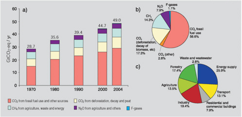
FIGURE 5-1 Global anthropogenic greenhouse gas (GHG) emissions. (a) Global annual emissions of anthropogenic GHGs from 1970 to 2004; (b) share of different anthropogenic GHGs in total emissions in 2004 in terms of CO2-equivalent; and (c) share of different sectors in total anthropogenic GHG emissions in terms of CO2-equivalent (forestry includes deforestation.). SOURCE: IPCC 2007a, p. 5, Fig. SPM.3. Reprinted with permission; copyright 2007, Intergovernmental Panel on Climate Change.
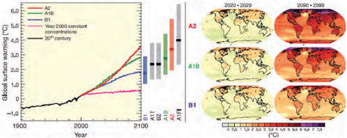
FIGURE 5-2 Atmosphere-Ocean General Circulation Model (AOGCM) projections of surface warming. Left panel: Solid lines are multimodel global averages of surface warming (relative to 1980-1999) in the IPCC Special Report on Emission Scenarios (SRES) A2, A1B, and A1, shown as continuations of the 20th century simulations (IPCC 2000). The orange line is for the experiment where concentrations were held constant at year 2000 values. The bars in the middle of the figure indicate the best estimate (solid line within each bar) and the probable range assessed for the six SRES marker scenarios at 2090-2099 relative to 1980-1999. The assessment of the best estimate and probable ranges in the bars includes the AOGCMs in the left part of the figure, as well as results from hierarchy of independent models and observational constraints. Right panels: Projected temperature changes for the early and late 21st century relative to the period 1980-1999. The panels show the multi-AOGCM average projections for the A2 (top), A1B (middle), and B1 (bottom) SRES averaged over decades 2020-2029 (left) and 2090-2099 (right). SOURCE: IPCC 2007b, p. 14, Figure SPM.5; Right Panel: IPCC 2007b, p. 15, SPM.6. Reprinted with permission; copyright 2007, Intergovernmental Panel on Climate Change.
IPCC Mitigation Findings
The IPCC concluded that the impacts of climate change can be reduced, delayed, or avoided through mitigation strategies designed to stabilize atmospheric carbon concentrations. These concentrations can be stabilized primarily by reducing anthropogenic carbon emissions and, secondarily, by increasing carbon sinks (see Table 5-1). Figure 5-3 depicts the future carbon emission profiles needed to achieve the various stabilization concentrations and the global mean temperature associated with each stabilization concentration. The IPCC strongly suggests that the technology needed to achieve the needed stabilization levels is already or will very soon be available. They also claim that 60-80% of the needed emission reductions would have to come from the energy sector, via a shift to noncarbon-based energy sources and energy efficiency (IPCC 2007a,d)
In response to a request from Congress, the National Research Council (NRC) has undertaken America’s Climate Choices (ACC), a suite of studies designed to inform and guide responses to climate change across the nation. A final ACC report, addressing strategies to reduce or adapt to the impacts of climate change, is expected to be complete in 2010.
Overview of Quantification Methods, Key Uncertainties, and Sensitivities
Defining the Marginal Damage of GHG Emissions
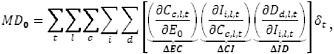
The combustion of fossil fuels is a major source of GHG emissions, which create externalities through their impact on the stock of GHGs in the atmosphere and the subsequent effects of GHG concentrations on climate. Evaluating the external costs of energy due to climate change is a daunting task. The principal difficulty is the complexity arising from the fundamental dimensionality of the climate problem. The relevant dimensions are time (indexed by t), location (indexed by l), the set of relevant climatic variables (indicated by the index c), the categories of physical impacts as a result of climate changes (indexed by i), and the categories of damage incurred by these impacts (indexed by d). The external cost of an additional ton of GHGs, E0, emitted at time t = 0 depends on the following:
-
The effect of emissions on Earth-system processes and, in turn, climatic variables in candidate locations over future time periods, Cc,l,t.
-
The contemporaneous effect of climate changes in each location on various categories of physical impacts, Ii,l,t.
-
The contemporaneous effect of impacts in each location on various categories of damage, Dd,l,t.
TABLE 5-1 Characteristics of Post-Third Assessment Report (TAR) Stabilization Scenarios and Resulting Long-Term Equilibrium Global Average Temperature and the Sea-Level Rise Component from Thermal Expansion Only
|
Category |
CO2 Concentration at Stabilization (2005 = 379 ppm)b |
CO2-Equivalent Concentration at Stabilization Including GHGs and Aerosols (2005 = 375 ppm)b |
Change in Global CO2 Emissions in 2050 (Percent of 2000 Emissions)a,c |
Global Average Temperature Increase above Preindustrial Level at Equilibrium, Using “Best Estimate” Climate Sensitivityd,e |
Global Average Sea-Level Rise above Preindustrial Level at Equilibrium from Thermal Expansion Onlyf |
Number of Assessed Senarios |
|
|
|
ppm |
ppm |
Year |
Percent |
°C |
Meters |
|
|
I |
350-400 |
445-490 |
2000-2015 |
−85 to −50 |
2.0-2.4 |
0.4-1.4 |
6 |
|
II |
400-440 |
490-535 |
2000-2020 |
−60 to −30 |
2.4-2.8 |
0.5-1.7 |
18 |
|
III |
440-485 |
535-590 |
2010-2030 |
−30 to +5 |
2.8-3.2 |
0.6-1.9 |
21 |
|
IV |
485-570 |
590-710 |
2020-2060 |
+10 to +60 |
3.2-4.0 |
0.6-2.4 |
118 |
|
V |
570-660 |
710-855 |
2050-2080 |
+25 to +85 |
4.0-4.9 |
0.8-2.9 |
9 |
|
VI |
660-790 |
855-1130 |
2060-2090 |
+90 to +140 |
4.9-6.1 |
1.0-3.7 |
5 |
|
aThe emission reductions to meet a particular stabilization level reported in the mitigation studies assessed here might be underestimated because of missing carbon-cycle feedbacks. bAtmosphere CO2 concentrations were 379 parts per million (ppm) in 2005. The estimate of total CO2-equivalent concentration in 2005 for all long-lived greenhouse gases (GHG) is about 455 ppm, and the corresponding value including the net effect of all anthropogenic forcing agents is 375 ppm CO2-eq. cRanges correspond to the 15th to 85th percentile of the post-TAR scenarios distribution. CO2 emissions are shown so multigas scenarios can be compared with CO2-only scenarios. dThe best estimate of climate sensitivity is 3°C. eNote that global average temperature at equilibrium is different from expected global average temperature at the time of stabilization of GHG concentrations due to the inertia of the climate system. For the majority of scenarios assessed, stabilization of GHG concentrations occurs between 2100 and 2150. fEquilibrium sea-level rise is for the contribution from ocean thermal expansion only and does not reach equilibrium for at least many centuries. These values have been estimated using relatively simple climate models (one low-resolution AOGCM [Atmosphere-Ocean General Circulation Model] and several EMICs [Earth System Models of Intermediate Complexity] based on the best estimate of 3°C climate sensitivity) and do not include contributions from melting ice sheets, glaciers, and ice caps. Long-term thermal expansion is projected to result in 0.2 to 0.6 m per degree Celsius of global average warming above preindustrial levels. SOURCE: IPCC 2007a, p. 20, Table SPM.6. Reprinted with permission; copyright 2007, Intergovernmental Panel on Climate Change. |
|||||||
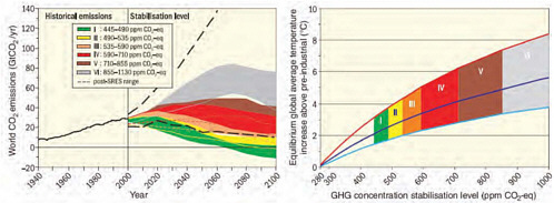
FIGURE 5-3 Global CO2 emissions for 1940 to 2000 and emission ranges for categories of stabilization scenarios from 2000 to 2100 (left panel); and the corresponding relationship between the stabilization target and the probable equilibrium global average temperature increase above preindustrial levels (right panel). Approaching equilibrium can take several centuries, especially for scenarios with higher levels of stabilization. Colored shadings show stabilization scenarios grouped according to different targets (stabilization categories I to VI). The right-hand panel shows ranges of global average temperature change above preindustrial levels, using (i) “best-estimate” climate sensitivity of 3°C (black line in middle of shaded area), (ii) upper bound of probable range of climate sensitivity of 4.5°C (red line at top of shaded area), and (iii) lower bound of probable range of climate sensitivity of 2°C (blue line at bottom of shaded area). Black dashed lines in the left panel give the emissions range of recent baseline scenarios published since IPCC (2000). Emission ranges of the stabilization scenarios comprise CO2-only and multigas scenarios and correspond to the 10th to 90th percentile of the full scenario distribution. NOTE: CO2 emissions in most models do not include emissions from decay of above-ground biomass that remains after logging and deforestation and from peat fires and drained peat soils. SOURCE: IPCC 2007a, p. 21, Figure SPM.11. Reprinted with permission; copyright 2007, Intergovernmental Panel on Climate Change.
The dependence can be summarized in Equation 5-1, which is the analogue of the impact-pathway approach used in the analysis in Chapters 2 and 3:
Equation 5-1
where δt = (1 + r)–t is a factor that discounts damages in future year t back to the present, and r is the rate of discount. Effect b is captured by the term ∆CI, which summarizes the results of physical impact models. These models suggest how changes in temperature and precipitation may affect agricultural yields or how changes in climate will affect biodiversity. Effect c is captured by the term ∆ID, which captures the monetary damages associated with changes in agricultural yields or loss of species diversity. Attempts to measure these damages are reviewed briefly later in this section. In many cases, the relationships between climate impacts and damages are based on judgment, assumptions, or analogy because data are lacking.
This last point highlights the second difficulty facing any assessment of the costs of climate change: lack of information and uncertainty regarding effects a-c. The terms represented by ∆EC, which include the extent of ice sheet melting and shifts in regional distribution of precipitation are still subject to considerable uncertainty. A vast amount of effort is actively being dedicated to elaborating the elements of ∆CI. However, while natural scientists mostly agree on the climatic variables whose impacts should be studied, there is less consensus on what impacts are significant and should be examined. Moreover, even those impacts thought to be significant (for example, species loss) respond to changes in climate in ways that are poorly understood. The difficulties in estimating monetary damages are described in more detail below.
The climate equivalent of the Air Pollution Emission Experiments and Policy (APEEP) model would embody estimates of ∆EC, ∆CI, and ∆ID and combine them according to Equation 5-1 to produce a summary measure of marginal damage. The committee did not have access to an integrated assessment model (IAM) of this kind. Indeed, such a model does not exist—the IAMs used for climate studies are designed not to produce descriptively realistic, spatially disaggregate responses of climatic impact and damage variables but rather to bring together key stylized facts about these responses within the framework of Eq. 5-1 as a means of elucidating their joint implications. The benefits of such integration are often gained at the expense of introducing substantial theoretical and empirical weaknesses into IAMs. Although each element of ∆EC, ∆CI, and ∆ID can be thought of as a model in its own right, IAMs adopt reduced-form approaches, which
reduce these complex relationships into simplified response surfaces, in the process oversimplifying the complexities of the underlying science. In addition, IAMs typically cope with the curse of dimensionality by considering only relatively narrow sets of impacts or types of damage. IAMs also tend to trade off coarse regional coverage in favor of broad global scope, so relationships validated for restricted geographic domains are implicitly scaled up to broader spatial scales. The remainder of this section describes in general terms how IAMs, such as the Regional Integrated Model of Climate and the Economy (RICE) and the Dynamic Integrated Model of Climate and the Economy (DICE), the Climate Framework for Uncertainty, Negotiation, and Distribution (FUND) model, and the Policy Analysis of the Greenhouse Effect (PAGE) model, evaluate marginal damages. In a typical IAM, the marginal damages from a ton of CO2-eq emissions (E) emitted today (year 0) can be expressed as
Equation 5-2
where
t = year of impact,
MD0 = marginal damage from GHG emissions in year 0 ($/ton CO2-eq),
Tt = mean global temperature in year t relative to preindustrial levels (°C),
E0 = GHG emissions in year 0 (ton CO2-eq),
Dt = total climate damages in year t ($),
δt = discount factor from year t to 0 = (1 + r)–t, where r is the discount rate, and
tf = final year for which climate damages are included.
The expression indicates that the marginal damages from GHG emissions (MD) depend on how much temperatures increase in response to a unit increase in emissions (dT/dE), how much additional climate damage results from this temperature increase (dD/dT), how one values future damages relative to the present (δ), and how far into the future one aggregates impacts (tf). In terms of the preceding discussion, climate effects have been reduced to temperature, and the link between climate and impacts and impacts and damages has been condensed into a single step.
The relationship between a ton of CO2-eq emitted today and future temperature depends on the effects of GHG emissions on the concentration of GHGs in the atmosphere, and on the effects of GHG concentrations on temperature. Spatially detailed predictions of the impact of GHG concentrations on temperature and precipitation are provided by general circulation
models. IAMs typically simplify these relationships and describe changes in mean global temperature corresponding to a ton of CO2-eq emissions.
In the most disaggregated IAMs, the monetary damages associated with a change in temperature are calculated by estimating damages by sector (for example, energy, health, and agriculture) and geographic region. Damages are expressed as a percentage of GDP using methods described in the next subsection: Approach to Measuring Marginal Damages in Integrated Assessment Models. dDt/dTt represents the aggregation of impacts across sectors and regions. How change in GDP are aggregated across regions—whether using equity weights or by summing the monetary changes in GDP—is discussed below.
Future monetary damages are discounted either at the market rate of interest (the revealed preference approach), or using the Ramsey formula (the prescriptive approach), which describes how the discount rate, r, varies along an optimal growth path (see Pearce et al. 2003). These two approaches are discussed in detail later in the chapter. Marginal damages are extremely sensitive to the choice of discount rate, given the fact that the climate impacts of a ton of CO2-eq emissions will be felt for centuries (tf is typically 100 to 300 years).
The marginal-damage formula in Equation 5-2 assumes that the effect of a ton of CO2-eq emissions on temperature and the effects of temperature on the economy are certain—which are clearly not the case. Indeed, a major difference between quantifying the local air pollution effects of fossil fuels and the impacts of GHG emissions is that the two differ significantly in their time dimension, their spatial scale, the variety of impacts, and, hence, in the certainty with which they can be estimated. In contrast to SO2 or NOx, CO2 is a pollutant that resides in the atmosphere for centuries.4 This factor implies that the effects of a ton emitted today must be estimated on a time scale (centuries) in which the state of the world is inherently more uncertain than the period during which effects of local air pollutants are estimated (months or years). Key sensitivities in Equation 5-2 include the impact of a change in atmospheric concentrations of CO2 on temperature (termed climate sensitivity) and how dD/dT varies with T. There is, in reality, a distribution of damages associated with any given temperature change.
IAMs typically handle this uncertainty in two ways. One is to calculate marginal damages using Monte Carlo analysis: Parameters used for dT/dE and dD/dT are drawn from probability distributions and used to calculate the corresponding distribution of marginal damages. A second approach is to acknowledge that, corresponding to each change in mean global temperature from pre-industrial levels, there is a probability of
abrupt, catastrophic events, such as the melting of the West Antarctic ice sheets or melting of permafrost—events that could result in huge declines in world GDP. Some models attempt to estimate what individuals would pay to avoid such events. The next section provides an overview of how the damages associated with various temperature changes are modeled in three prominent IAMs.
Approach to Measuring Marginal Damages in Integrated Assessment Models
IAMs combine simplified global climate models with economic models in an effort to estimate the economic impacts of climate change and to identify emission paths that balance these economic impacts against the costs of reducing GHG emissions. Three of the most widely used IAMs are RICE and DICE (W. Nordhaus, Yale University), FUND (R.S.J. Tol, Economic and Social Research Institute, Dublin, Ireland), and PAGE (C. Hope, University of Cambridge). The goal of this section is to provide overviews of how each of these IAMs monetizes the impact of changes in mean global temperature.
RICE and DICE Models
These models examine the links between economic growth, CO2 emissions, the carbon cycle, the economic damages associated with climate change, and climate-change policies. These models incorporate the climate system’s “natural capital” into a model based on traditional economic growth theory. They treat as exogenous global population, global stock of fossil fuels, and the pace of technological change, and they calculate world output and capital stock, CO2 emissions and concentrations, global temperature change, and climate damages. RICE distinguishes various regions of the world (8 in some versions; 13 in others), and DICE has a single, aggregated global economy. The models are typically run from 1990 until 2100.
The approach to quantifying climate-change damages in each sector in RICE is as follows: (1) The percentage reduction in GDP associated with a mean global temperature increase of T is calculated for the year 1995 for each sector (i) and region (j). (Call this Qij(T).) (2) The impact of the T °C temperature change is calculated for a future year, t, by multiplying Qij(T) by the ratio of per capita GDP in year t to per capita GDP in 1995 raised to a power η, where η is the income elasticity of the impact index. The percentage change in GDP in year t for temperature change T is thus,
Equation 5-3
In practice Qij(T) is calculated for benchmark warming—a 2.5°C increase in mean global temperature—based on a review of the literature. η is determined from a literature review or expert opinion. Qij(T) changes as a function of T according to a quadratic function. The sectors for which impacts are monetized in RICE and DICE are agriculture, sea-level rise, other market sectors, health, nonmarket amenities, human settlements and ecosystems, and catastrophic damages. The magnitudes of damages in these sectors are discussed in sections below.
FUND Model
The Climate Framework for Uncertainty, Negotiation, and Distribution (FUND) model examines how a set of exogenous scenarios concerning economic growth, population growth, energy-efficiency improvements, decarbonization of energy use, and GHG emissions affect the concentration of atmospheric CO2, global mean temperature, and the impacts of temperature change. FUND models these links for nine regions5 over 250 years (1950 to 2200).
The sectors for which impacts are monetized in FUND are agriculture, forestry, water resources, energy consumption, sea-level rise, ecosystems, and human health. Monetization of impacts in FUND is slightly different for each sector and more detailed than the reduced-form approach used in RICE and DICE. For example, the impact of a temperature change on agricultural revenues consists of three components: One reflects the difference between future temperature and ideal growing temperature for the region; a second reflects the rate of increase in temperature, which captures opportunities for adaptation; and the third component reflects the carbon fertilization effect. To map the percentage change in agricultural revenues implied by these three effects into a change in GDP requires estimates of the share of agriculture in GDP. These estimates, in turn, are modeled as a function of per capita GDP and assumptions about the income elasticity of agriculture.
FUND differs from RICE and DICE in that the base year impacts in agriculture and ecosystems depend not only on the magnitude of temperature change but also on the rate of temperature change. It is also the case in FUND that the effect of a change in mean global temperature on marginal damages varies by sector
PAGE Model
The Policy Analysis of the Greenhouse Effect (PAGE) model is a multiregional model that models the impacts of climate change in three sectors—economic impacts, noneconomic impacts, and discontinuity impacts—that is, impacts associated with abrupt changes to the climate system.6 Functions that describe the economic and noneconomic impacts of a given temperature change (T) in region r are of the form
Equation 5-4
where I(r) is the percentage change in GDP associated with the impact, A(r) is a scaling factor and n(r) lies between 1 and 3. The weights A(r) represent the percent of GDP lost in region r relative to losses in the European Union. For a description of the modeling of discontinuity impacts see Hope (2006).
IMPACTS ON PHYSICAL AND BIOLOGICAL SYSTEMS
Earth’s climate system is integrally intertwined with many other global biological, chemical, and physical systems. Impacts on the weather, cryosphere, hydrosphere, coastal zones, and the biosphere are briefly discussed below. Impacts on human systems resulting from impacts on these physical systems are discussed in more detail in a subsequent section. This discussion is intended to provide a brief summary of recent knowledge. Another effort is under way within the NRC to study issues relating to global climate change.7 It is important to keep in mind that none of the individual impacts described in this section have been monetized.
Changes in the Weather
The most literal effect of climate warming is an increase in ambient air temperatures, particularly at night over land in the Northern Hemisphere (Figure 5-2). Global climate models predict an increase in the frequency of heat waves, heavy precipitation events, and the intensity of tropical cyclones (IPCC 2007b). The IPCC also predicts that precipitation will likely decrease in the subtropics and will very likely increase near the poles (Figure 5-4).
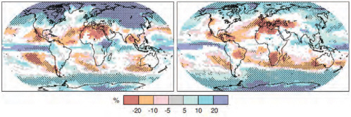
FIGURE 5-4 Multimodel projected patterns of precipitation changes. Relative changes in precipitation (in percentage) for the period 2090-2099, relative to 1980-1999. Values are multimodel averages based on the IPCC Special Report on Emission Scenarios (SRES) A1B for December to February (left) and June to August (right). White areas are where less than 66% of the models agree in the sign of the change, and stippled areas are where more than 90% of the models agree in the sign of the change. SOURCE: IPCC 2007b, P.16, Figure SPM.7. Reprinted with permission; copyright 2007, Intergovernmental Panel on Climate Change.
Changes in the Cryosphere
The cryosphere, comprising all the permanent and seasonal snow and ice formations found on Earth, including the polar ice caps, sea ice, permafrost, glaciers, and seasonal snow and ice on land and water, is particularly sensitive to climate change, and a dramatic decrease is predicted in the amount of snow and ice on Earth as climate changes progress. In fact, scientists have already documented the following changes (Rosenzweig et al. 2007):
-
The Arctic sea-ice extent has declined by about 10% to 15% since the 1950s, and the 2007 summer minimum is more than 35% smaller than the 1950-1980 average.
-
Mountain glaciers have receded on all continents.
-
Northern Hemisphere permafrost is thawing.
-
Snowmelt and runoff have occurred increasingly earlier in Europe and western North America since the late 1940s.
-
The annual duration of lake- and river-ice cover in Northern Hemisphere mid- and high latitudes has been reduced by about 2 weeks and become more variable.
IPCC (2007b) also predicts the complete disappearance of late-summer Arctic sea ice by the end of the 21st century.
Changes in the Hydrosphere
The hydrosphere comprises all the liquid water systems on Earth, including the oceans, lakes, rivers, streams, and aquifers. The hydrosphere is tightly integrated with the climate system and the cryosphere. Climate change and consequent warming are linked to changes in the hydrologic cycle with increased evaporation from land and seas, changing precipitation patterns, and reduced snow cover. Specific observed changes in the hydrosphere include the following (Rosenzweig et al. 2007):
-
The salinity of the North Atlantic is decreasing, most likely because of melting glaciers.
-
Annual runoff is increasing in higher latitudes and decreasing in some parts of West Africa, southern Europe, and southern Latin America.
-
Peak spring river flows are occurring earlier in areas with a seasonal snow pack. This causes less water to be available during the late summer and autumn when human and ecological demand tends to be the greatest.
-
The temperature, chemistry, and ultimately the structure of lakes and rivers are changing.
-
‘Large’ floods are occurring with more frequency around the globe.
-
Very dry areas have more than doubled since 1970, causing desertification and droughts.
Ultimately, between the changes in weather patterns and changes in the cryosphere and hydrosphere, scientists predict that Earth will become dryer in the subtropics, especially in the Northern Hemisphere, and much wetter and less frozen near the poles. In other words, climate change is likely to manifest in ways, with consequent impacts, that will not occur evenly across the globe. Global climate models (GCMs) predict increasing global precipitation, with important regional variation, including increases in high latitudes and parts of the tropics but decreases throughout the subtropics (Bates et al. 2008). The western United States, for example, is vulnerable to reduced water availability. Table 5-2 lists climate-related changes in the freshwater system presented in the fourth assessment report of the IPCC.
The physical impacts on water availability vary considerably geographically; some regions benefit from warming while other areas suffer. For example the Warren et al. (2006a) analysis shows water scarcity increasing on a global scale from 29% in 1995 to 39% in 2085 under the A1 and B1 scenarios, respectively, shown in Figure 5-2. Some areas see sharper increases in water scarcity under their analysis (South Asia more than doubles from 26% to 59%) while other areas see a decline in water scarcity (Europe falls from 38% to 26%). The United States and Canada see a modest increase in scarcity from 16% to 20% in their analysis.
Changes in the Coastal Zones
Rising sea levels—among the best-documented impacts of climate change—are another consequence of the melting cryosphere. Sea level has been rising at the rate of 1.7 to 1.8 mm/yr over the past century. This rate increased to approximately 3 mm/yr over the past decade (IPCC 2007a). Rising sea levels and increased storm intensities are rapidly eroding coastlines around the globe. Seventy-five percent of the east coast of the United States and 67% of the east coast of the United Kingdom are thus affected (Rosenzweig et al. 2007). However, there is scientific consensus that over many centuries thermal expansion of the ocean due to global warming is very likely to cause much larger rises in sea levels than those observed over the 20th century. In the latest IPCC projections, thermal expansion contributes 70-75% of the best estimate of sea-level rise for each of the six IPCC Special Report on Exposure Scenarios (SRES) marker scenarios, in
TABLE 5-2 Climate-Related Observed Trends of Various Components of the Global Freshwater Systems
|
|
Observed Climate-Related Trends |
|
Precipitation |
Increasing over land north of 30°N over the period of 1901-2005 Decreasing over land between 10°S and 30°N after the 1970s (WGI AR4, Chapter 3, Executive Summary) Increasing intensity of precipitation (WGI AR4, Chapter 3, Executive Summary) |
|
Cryosphere |
|
|
Snow cover |
Decreasing in most regions, especially in spring (WGI AR4, Chapter 4, Executive Summary) |
|
Glaciers |
Decreasing almost everywhere (WGI AR4, Chapter 4, Section 4.5) |
|
Permafrost |
Thawing between 0.02 m/yr (Alaska) and 0.4 m/yr (Tibetan Plateau) (WGI AR4, Charter 4, Executive Summary; WGII AR4, Chapter 15, Section 15.2) |
|
Surface Waters |
|
|
Streamflow |
Increasing in Eurasian Arctic, significant increases or decreases in some river basins (WGII AR4 Chapter 1, Section 1.3.2) Earlier spring peak flows and increased winter base flows in Northern America and Eurasia (WGII AR4, Chapter 1, Section 1.3.2). |
|
Evapotranspiration |
Increased actual evapotranspiration in some areas (WGI AR4, Chapter 3, Section 3.3.3). |
|
Lakes |
Warming, significant increases or decreases of some lake levels, and reduction in ice cover (WGII AR4, Chapter 1, Section 1.3.2). |
|
Groundwater |
No evidence for ubiquitous climate-related trend (WGII AR4, Chapter 1, Section 1.3.2) |
|
Floods and Droughts |
|
|
Floods |
No evidence for climate-related trend (WGII AR4, Chapter 1, Section 1.3.2), but flood damages are increasing (WGII AR4, Chapter 3, Section 3.2) |
|
Droughts |
Intensified droughts in some drier regions since the 1970s (WGII AR4, Chapter 1, Section 1.3.2; WGI AR4, Chapter 3, Executive Summary) |
|
Water quality |
No evidence for climate-related trend (WGII AR4, Chapter 1, Section 1.3.2) |
|
Erosion and sediment transport |
No evidence for climate-related trend (WGII AR4, Chapter 3, Section 3.2) |
|
Irrigation water demand |
No evidence for climate-related trend (WGII AR4, Chapter 3, Section 3.2) |
|
NOTES: WGI AR4, Chapter 3, Trenberth et al. 2007; WGI AR4, Chapter 4, Lemke et al. 2007; WGII AR4, Chapter 1, Rosenzweig et al. 2007; WGII AR4, Chapter 3, Kundzewicz et al. 2007; and WGII AR4, Chapter 15, Anisimov et al. 2007. SOURCE: Kundzewicz et al. 2007, p.177, Table 3.1. Reprinted with permission; copyright 2007, Intergovernmental Panel on Climate Change. |
|
the most extreme case exhibiting a 5-95% confidence interval of 0.26-0.59 m by the year 2100 (IPCC 2007b, p. 820, Table 10.7; IPCC 2007b, p. 821, Figure 10.33). This projection is cause for concern, given that relative sea-level rises have exceeded 8 inches in some areas along the Atlantic and Gulf coasts (see Karl et al. 2009, p. 37, figure) Although the contributions to sea-level rise made by thermal expansion and melting glaciers are well understood, uncertainty remains about the magnitude of the ice sheets’ effects, so much so that their impact was left unquantified in the most recent IPCC report. On the basis of several recent studies on sea-level rise, Karl et al. (2009) concluded that the IPCC predictions are likely to underestimate the impact and cite estimates by century’s end of 0.9-1.2 m under higher emission scenarios, with an upper bound of 2 m.
Changes in the Biosphere
Many plants and animals have relatively specific environmental conditions in which they can survive. Even small environmental changes, such as extremes in ambient temperature, or the availability of water, can make a region inhospitable to members of the existing flora and fauna. Ecologists are already documenting important shifts in ecosystem structures and functioning, such as the following (Rosenzweig et al. 2007):
-
Plant and animal ranges have shifted to cooler higher latitudes and altitudes. Therefore, as overall temperatures rise, plants and animals with very narrow temperature requirements will shift their ranges accordingly or become extirpated.
-
The timing of many life-cycle events, such as flowering, migration, and emergence, has shifted to earlier in the spring and often later in the autumn.
-
Different species change at different speeds and in different directions, causing a changing of species interactions (for example, predator-prey relationships).
IMPACTS ON HUMAN SYSTEMS
Observed (and predicted) changes in Earth’s global systems have significant ramifications for humans. The redistribution of water availability across the globe, for example, will amplify water conflicts, particularly in regions that are getting drier. Changes in the availability of water and in the length of growing seasons will affect which crops farmers can plant and how much those crops yield. Tropical diseases will start to affect more people as the ranges of disease vectors, such as mosquitoes, shift pole-ward.
Table 5-3 describes some of the many ways in which climate change may affect important human systems.
The impacts of climate change on humans will not be uniform throughout the world. Different regions will experience climate change somewhat differently. Southern Africa, for example, is predicted to become drier and will therefore need to cope with water scarcity. Northern Europe, on the other hand, is predicted to become wetter. Figure 5-5 summarizes some of the key regional impacts humans will experience. The rest of this section systematically explores the impacts of climate change on a variety of aspects of human life, including water resources; ecosystem services; food production and forest products; sea-level rise and coastal populations; and human health, industry, society, and security.
Water Availability
A critical challenge facing the growing world population is access to water, which could be significantly affected by climate change. Warren et al. (2006a) noted that a country experiences water scarcity when available supply falls below 1,000 m3 per person per year and absolute scarcity when supply falls below 500 m3 per person per year. Globally, they estimate that roughly 30% of the world’s population was “water stressed” (defined as experiencing water scarcity) in 1995 (Warren et al. 2006a, Table A2). By 2085, they project that 39-59% of the world’s population could be water stressed, depending on economic and population growth. However, all analyses and predictions of physical impacts must be qualified by the great uncertainties about hydrologic cycles and their responses to warming. Additional caveats to estimates of impacts are the possibilities of adaptation and mitigation. For example, exposure to water scarcity will change as populations migrate for reasons related or unrelated to global warming.
Changes in water availability can lead to losses in crop production, premature deaths, and greater disease prevalence from water shortages in the short run and adjustment costs of population movements as people abandon areas that have become too dry and as people engineer new water transfers. However, measuring the impacts of increasing water scarcity is difficult. Among other issues, the value of losses is exacerbated by increasing demand for irrigation in agriculture (Mendelsohn and Williams 2007). Aldy et al. (2009) provide summaries of damages from climate change as measured in a number of studies. Table 5-4 reports estimates of damages arising from changes in water availability. These damages are reported as percentages of GDP at the end of this century. For the United States, damages range from a low of .01% to .03% for warming between 4.6 and 7.1°C to a high of .29% for 2.5°C.
TABLE 5-3 Examples of Possible Impacts of Climate Change Due to Changes in Extreme Weather and Climate Events, Based on Projections to the Mid- to Late 21st Century
|
Phenomenona and Direction of Trend |
Likelihood of Future Trends Based on Projections for 21st Century Using SRES Scenarios |
Examples of Major Projected Impacts by Sectors |
|
Agriculture, Forestry, and Ecosystems (WGII 4.4, 5.4) |
||
|
Over most land areas, warmer and fewer cold days and nights, warmer and more frequent hot days and nights |
Virtually certainb |
Increased yields in colder environments; decreased yields in warmer environments; increased insect outbreaks |
|
Warm spells and heat waves; frequency increases over most land areas |
Very likely |
Reduced yields in warmer regions due to heat stress; increased danger of wildfire |
|
Heavy precipitation events; frequency increases over most areas |
Very likely |
Damage to crops; soil erosion, inability to cultivate land due to waterlogging of soils |
|
Area affected by drought increases |
Likely |
Land degradation; lower yields and crop damage and failure; increased livestock deaths; increased risk of wildfire |
|
Intense tropical cyclone activity increases |
Likely |
Damage to crops; windthrow (uprooting) of trees; damage to coral reefs |
|
Increased incidence of extremely high sea level (excludes tsunamisc |
Likelyd |
Salinization of irrigation water, estuaries, and freshwater systems |
|
aSee WGI Table 3.7 for further details regarding definitions. bWarming of the most extreme days and nights each year. cExtreme high sea level depends on average sea level and on regional weather systems. It is defined as the highest 1% of hourly values of observed sea level at a station for a given reference period. dIn all scenarios, the projected global average sea level at 2100 is higher than it is in the reference period. The effect of changes in regional weather systems on sea level extremes has not been assessed (WGI 10.6). |
||
|
|
|
|
|
Water Resources (WGII 3.4) |
Human Health (WGII 8.2, 8.4) |
Industry, Settlement, and Society (WGII 7.4) |
|
Effects on water resources relying on snowmelt; effects on some water supplies |
Reduced human mortality from decreased cold exposure |
Reduced energy demand for heating; increased demand for cooling; declining air quality in cities; reduced disruption to transport due to snow and ice; effects on winter tourism |
|
Increased water demand; water quality problems, for example, algal blooms |
Increased risk of heat-related mortality, especially for the elderly, chronically sick, very young and socially isolated |
Reduction in quality of life for people in warm areas without appropriate housing; impacts on the elderly, very young. and poor |
|
Adverse effects on quality of surface and groundwater; contamination of water supply; water scarcity may be relieved |
Increased risk of deaths, injuries and infectious, respiratory and skin diseases |
Disruption of settlements, commerce, transport, and societies due to flooding; pressures on urban and rural infrastructures; loss of property |
|
More widespread water stress |
Increased risk of food and water shortage; increased risk of malnutrition; increased risk of water- and food-borne diseases |
Water shortage for settlements, industry, and societies; reduced hydropower-generation potentials; potential for population migration |
|
Power outages causing disruption of public water supply |
Increased risk of deaths, injuries, water- and foodborne diseases; post-traumatic stress disorders |
Disruption by flood and high winds; withdrawal of risk coverage in vulnerable areas by private insurers; potential for population migrations; loss of property |
|
Decreased freshwater availability due to saltwater intrusion |
Increased risk of deaths and injuries by drowning in floods; migration-related health effects |
Costs of coastal protection versus costs of land-use relocation; potential for movement of populations and infrastructure |
|
ABBREVIATION: SRES = Special Report on Emission Scenarios. SOURCE: IPCC 2007d, p.18, Table SPM.1. Reprinted with permission; copyright 2007, Intergovernmental Panel on Climate Change. |
||
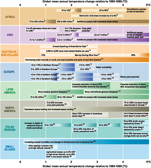
FIGURE 5-5 Examples of regional impacts of climate change. SOURCE: Yohe et al. 2007, p. 829, Table 20.9.
World damages are modestly higher. Tol (2002a) reported the highest damages of .43% for 1°C warming. The range of estimates for the United States and for the world is great, especially when taking into account the different assumptions about global warming. This range speaks to the difficulties in making sharp impact predictions.
Regarding the three IAMs described earlier in the chapter, PAGE does not provide sector-specific estimates of damages, and RICE and DICE do not provide separate estimates for water resources. Indeed, Nordhaus and
TABLE 5-4 Water Availability Effects from Climate Change for Selected Studiesa (Percentage of Contemporaneous GDP Around 2100)
|
|
Cline 1992 |
Fankhauser 1995a |
Mendelsohn and Neumann 1999 |
Mendelsohn and Williams 2004 |
Mendelsohn and Williams 2007 |
Titus 1992 |
Tol 1995 |
Tol 2002a |
|
Warming, Cb |
2.5 |
2.5 |
2.5 |
4.6-7.1 |
2.5-5.2 |
4.0 |
2.5 |
1.0 |
|
United States |
.12 |
.29 |
.07 |
.01-.03 |
.20 |
n/a |
.07 |
|
|
World |
n/a |
.24 |
n/a |
.01-.03 |
.00-.02 |
n/a |
n/a |
.43 |
|
NOTES: n/a = values not available or not estimated. In some cases, estimates for the United States also include Canada. aStern (2007) does not separate out individual categories within market and nonmarket impacts. bWarming is relative to preindustrial (as opposed to current) temperatures. SOURCE: Adapted from Aldy et al. 2009, with permission from the authors. |
||||||||
Boyer (1999, p. 4-13) argued that the damages from water availability can be set to zero, based on their survey of previous studies. The FUND model 3.0 measures water availability impacts for each of 16 regions using the following formula:
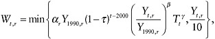
Equation 5-5
where
W = denotes the change in water resources in 1995 dollars in region r in year t,
Y = denotes income (in 1995 dollars),
T = global mean temperature,
α = benchmarking parameter,
τ = parameter measuring technological progress in water supply and demand (ranges from 0 to .01 with a preferred estimate of .005,
β = elasticity of impact with respect to income growth (ranging from .7 to 1 with a preferred estimate of .85),
γ = elasticity of impact with respect to temperature change (ranging from .5 to 1.5 with a preferred estimate of 1).
The parameter choices are made by calibrating the FUND model to results from Downing et al. (1995, 1996a). The estimated impact of a 1°C increase in global temperature is −0.065% of GDP for the United States (FUND 2008, p. 33, Table EFW). A negative estimate indicates benefits to the United States from warming. This estimate is imprecisely estimated with a coefficient of variation equal to 1.0. The impact on other regions is small with a few exceptions. The former Soviet Union sees benefits as large as 2.75% of GDP, while China has losses of 0.57% of GDP. Overall, however, losses are small, and in all cases, the estimates have very large standard errors.
Coastal Zone Impact of Climate Change
As previously mentioned, the coastal sector is one of best-documented areas of the impacts of climate change. However, it is difficult to assess with any confidence what the monetary damages of elevated seas might be for the United States, let alone globally. The only comprehensive assessment of the vulnerability of the U.S. coastline to sea-level rise (Thieler and HammarKlose 1999; 2000a,b) predates the latest IPCC estimates. Notwithstanding that, the fact that their methodology of assigning to segments of coastline an index of vulnerability calculated on the basis of rank-ordered attributes would suggest that updated data on sea-level rise will preserve the relative position of the coastline in the vulnerability hierarchy, at least over broad geographic scales.8 Recent analyses at the regional scale indicate that sandyshore environments, such as the Mid-Atlantic coastline, have a high likelihood of seeing more rapid erosion and segmentation of barrier islands, as well as wetland loss. For example, Figure 5-6 illustrates that for the Mid-Atlantic region an acceleration in sea-level rise of 2 mm/year over current rates will cause many wetlands to become stressed, while most wetlands probably will not survive a 7 mm/year acceleration (consistent with IPCC’s upper-bound estimate (see section above “Changes in the Coastal Zones”). The value of these kinds of losses has not been rigorously quantified. Depending on the increase in sea level, the adaptation options confronting human populations in the coastal zone are to protect the shore, relocate inland, or do a combination of both, each of which is associated with forgone income and well-being—that is, damage. How much of each option to be chosen is essentially an economic decision, which is simulated within IAMs in the process of arriving at aggregate estimates of climate damages. The remainder of this section sheds light on the methodological details of
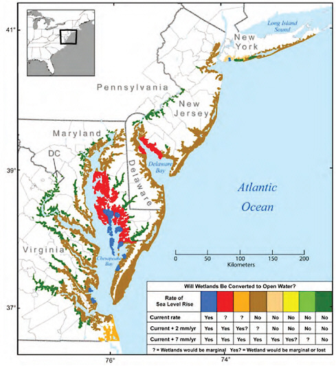
FIGURE 5-6 Mid-Atlantic wetland marginalization and loss as a consequence of sea-level rise. SOURCE: CCSP 2009, Fig. ES.2.
this process, as a way of illustrating the large extent to which it is driven by assumptions on the part of IAM modelers.
There is a sizeable literature on the damages associated with sea-level rise. The differences in model results stem from different ways of representing the processes by which damages arise, including the level of detail in climate- and physical-impact modeling and the choice between a “process-based” and “reduced-form” approaches to representing impacts. The RICE and DICE models (Nordhaus and Boyer 2000) are typical of the reduced-form approach, while the detailed representations of damages
in the FUND model (Tol 2002a,b) exemplify the process-based approach. Both authors develop damage estimates on a regional basis by extrapolating from studies of the United States and other countries, but to implement the process-based approach requires many more assumptions about the detailed impacts of sea-level rise and the character of affected individuals’ adaptation responses.
Damages in the RICE model are constructed by developing a benchmark estimate of the cost of the sea level increase arising from 2°C warming in the United States (0.1% of GDP) and then applying this estimate to other regions using an index of coastal sensitivity. The benchmark estimate for the United States includes damages to developed and undeveloped land and damages from storms. The index of coastal sensitivity is constructed by dividing the ratio of coastal area to total area for a given region by the ratio for the United States (see Table 5-5). The income elasticity of coastal damages is assumed to be 0.2.
TABLE 5-5 Values of the Benchmarking Parameter (α)
|
|
Coastal Impacta |
Coastal Index (% of GDP, 1990) |
α † (2.5°C Impact) |
|
United States |
1.00 |
0.10 |
0.11 |
|
China |
0.71 |
0.07 |
0.07 |
|
Japan |
4.69 |
0.47 |
0.56 |
|
Western Europe |
5.16 |
0.52 |
0.60 |
|
Russia |
0.94 |
0.09 |
0.09 |
|
India |
1.00 |
0.10 |
0.09 |
|
Other high income |
1.41 |
0.14 |
0.16 |
|
High-income OPEC |
0.52 |
0.05 |
0.06 |
|
Eastern Europe |
0.14 |
0.01 |
0.01 |
|
Middle income |
0.41 |
0.04 |
0.04 |
|
Lower-middle income |
0.94 |
0.09 |
0.09 |
|
Africa |
0.23 |
0.02 |
0.02 |
|
Low income |
0.94 |
0.09 |
0.09 |
|
Global |
|
|
|
|
Output weighted‡ |
|
|
0.32 |
|
Population weighted§ |
|
|
0.12 |
|
aRatio of fraction of area in coastal zone in country to that fraction in the United States. “Coastal zone” is defined as that part of the region that lies within 10 kilometers of an ocean. †Calibrated to impacts in the year 2100. ‡Output projections in 2100 from RICE model base case. §1995 population. SOURCE: Nordhaus and Boyer (2000: Tables 4-5 and 4-10). Reprinted with permission; copyright 2008, MIT Press. |
|||
For the FUND model, Tol (2002a,b) followed the method pioneered by Fankhauser (1995a,b) in estimating the costs of sea-level rise as the sum of the capital cost of structures for coastal protection and the cost of foregone services from “dry” and “wet” coastal land that is inundated. This method entails determining the optimal level of coastal protection, which determines the first component of cost and also the amount of coastal land that is inundated, for a given rise in sea level.
The cost of inundation of unprotected land depends on the extent of land loss and population displacement from the inundation. Tol estimates population displacement as the product of projected loss of dry lands and average population density and makes several assumptions about the destinations of the resulting migrants.9 The next step is to monetize these impacts. The unit values of lost dry and wet land in countries of the Organization for Economic Co-operation and Development (OECD) are assumed to be $4 million/km2 and $5 million/km2, respectively, and are extrapolated to other regions by adjusting them according to the inundation probability-weighted population density in the coastal zone and per capita income. For population displacement, Tol assumes a cost of emigration from an affected zone equal to three times per capita income and an immigration cost equal to 40% of the per capita income in the host country.10 The results are shown in Table 5-5.
The amount of land (percentage of the coast) that is protected is determined by comparing the costs and benefits of protection. Table 5-6 presents the optimal fraction of the coast protected by region, as well as the costs of that protection.
Impacts on Ecosystems and Ecosystem Services
Without a solid, broadly accepted set of standards for the value of ecosystems, the external costs of climate change assigned to ecosystem effects tend to get categorized in one of two ways. Based on the IAMs that do incomplete and preliminary accounting, the damages are generally quite low, sometimes barely enough to register in the overall cost accounting for climate-change impacts. Other studies based on ecosystem services often start from the proposition that ecosystem services are critical for the maintenance of healthy people, communities, and people. As a consequence, they tend to assign large but rarely quantified amounts to the external impacts of
TABLE 5-6 Benchmark Sea-Level Rise Estimates in FUND
climate change. The general inclination of stakeholders who take this position to assign zero or even negative discount rates creates the foundation for extraordinarily large damages. The steps to quantitatively test or reconcile these perspectives will probably be numerous and challenging.
Four widely used IAMs (RICE and DICE, MERGE (model for evaluating regional and global effects), FUND, and PAGE) all estimate damage from climate change on the basis of willingness to pay for ecosystem services. An alternative approach, which calculates the economic value lost from the ecosystem services degraded by climate change, is addressed in the Millennium Ecosystem Assessment (2010), although these results are not quantitative in the sense that the output is damage per ton of CO2. All the published representations of ecological damages from climate change are highly simplified. Willingness to pay is typically based on data from one or a few countries, often the United States, and then scaled to other countries on the basis of an assumed relationship with GDP.
In the RICE and DICE models, human settlements and ecosystems are treated together. They assume that the capital value of climate-sensitive human settlements and ecosystems ranges from 5% to 25% of regional output. For the United States, the number is 10%; for island countries, and for countries with sensitive ecosystems, the number is higher. Willingness to pay to avoid a 2.5°C temperature change is assumed to be equal to 1% of the capital value of the vulnerable system (Nordhaus and Boyer 1999).
|
Wetland Value (106 km2) |
Protection Costs (109$) |
Emigrants 106 |
Value 109$ |
Immigrants 106 |
Value 109$ |
Total Costs 109$/year |
|
5.4 (2.7) |
83 (74) |
0.13 (0.07) |
7.5 (5.3) |
0.0 (0.20) |
2.9 (2.1) |
1.6 (0.9) |
|
4.3 (2.2) |
136 (45) |
0.22 (0.10) |
8.2 (5.4) |
0.64 (0.32) |
3.1 (2.2) |
1.7 (0.5) |
|
5.9 (2.9) |
63 (38) |
0.04 (0.02) |
2.8 (2.0) |
0.18 (0.10) |
1.6 (1.2) |
0.8 (0.4) |
|
2.9 (1.5) |
53 (50) |
0.03 (0.03) |
0.7 (0.7) |
0.03 (0.03) |
0.0 (0.0) |
0.5 (0.5) |
|
1.3 (0.7) |
5 (3) |
0.05 (0.08) |
0.4 (0.6) |
0.04 (0.07) |
0.0 (0.0) |
0.0 (0.0) |
|
0.9 (0.5) |
147 (74) |
0.71 (1.27) |
3.9 (7.2) |
0.64 (1.14) |
0.5 (0.9) |
2.0 (0.9) |
|
0.3 (0.2) |
305 (158) |
2.30 (1.40) |
3.7 (2.9) |
2.07 (1.26) |
0.5 (0.4) |
3.3 (1.6) |
|
0.2 (0.1) |
171 (126) |
2.39 (3.06) |
2.5 (3.4) |
2.15 (2.75) |
0.3 (0.4) |
1.8 (1.30 |
|
0.4 (0.2) |
92 (35) |
2.74 (2.85) |
5.4 (6.3) |
2.47 (2.56) |
0.7 (0.8) |
1.1 (0.4) |
|
SOURCE: Tol 2002a. Reprinted with permission; copyright 2008, Environmental and Resource Economics. |
||||||
The elasticity of willingness to pay with respect to income is assumed to be equal to 0.1.
FUND does a separate calculation for 16 regions. The impact of warming on ecosystems in FUND is calculated as a “warm-glow” effect in which people are assumed to assign value to biodiversity and other ecosystem services, independent of whether they receive any concrete benefits from those services (Tol 1999). The value of the damage function rises with the fraction of biodiversity lost, with the amount of warming, and with per capita income in each region (Warren et al. 2006b).
Approaches based on the valuation of ecosystem services typically calculate the cost of replacing natural services with human or industrial alternatives. Many studies of the value of ecosystem services, however, do not explicitly assess the vulnerability of the ecosystem services to climate change. Schröter et al. (2005) looked at the vulnerability of ecosystem services to climate change in Europe, but they did not calculate an explicit cost impact. Naidoo et al. (2008) concluded that, for a large set of ecosystem services, they could reliably estimate values for only four and that the values of these four ecosystem services do not align well with areas targeted for biodiversity conservation. Brauman et al. (2007) reviewed a number of approaches to assessing ecosystem services and concluded that, whether or not the services are monetized, trade-offs among them can provide a useful set of tools for evaluating policy options. This approach is used by the Mil-
lennium Ecosystem Assessment, which assessed the impacts of four future scenarios (including climate change) on the basis of the number of ecosystem services, in each of four categories, expected to increase or decrease.
Overall, estimates of the impacts of economic damage to ecosystems from climate change are more conceptual and heuristic than quantitatively meaningful. The approaches that generate explicit numbers are simple and nonmechanistic approaches, starting with the studies of a small number of ecosystem services for one region or country at one level of economic development and the willingness to pay. Even if these studies were accurate, they should not be assumed to cover the full suite of climate-sensitive ecosystem services or to capture effectively the extrapolation of willingness to pay to other services, regions, or levels of economic activity. Finally, the sensitivity of the ecosystem services to climate is not well-known. These factors combine to define an approach that can be very useful for understanding aspects of the way the system works but that are unlikely to provide values that can be robustly used for studies that address multiple sectors of the economy. Approaches based on valuing ecosystem services sometimes generate numerical values, but sometimes they do not. The approaches based on valuing ecosystem services are not yet integrated in any of the main IAMs. Realizing such integration would represent an important conceptual advance in the credibility of the modeling, but it might not yield dramatic improvements in model accuracy or utility.
Impacts on Agriculture
The welfare effects of climate change on agriculture depend on the impacts of climate on crop yields and on how farmers adapt to the impacts. In many areas of sub-Saharan Africa, temperatures are predicted to exceed optimal temperatures for many crops currently grown, and even for crops that could be substituted for current crops. Yield losses will, however, be less when irrigation is possible. Farmers may also be able to reduce income losses from crops by raising cattle and thus diversifying their agricultural portfolios. In northern latitudes, yields are actually predicted to increase for many crops, and areas in which field crops, such as winter wheat, can be grown are likely to extend into higher latitudes. The magnitude of physical impacts, in addition to depending on adaptation to climate in the form of crop substitution and irrigation, will depend on the magnitude of the CO2 fertilization effect: Increased carbon in the atmosphere will increase yields by promoting photosynthesis and reducing plant water loss.11
To estimate the GDP impacts of the effects of climate change on agriculture, economists predict the impact of temperature and precipitation on agricultural revenues. These estimates are based primarily on cross-sectional studies—often referred to as the Ricardian approach (Mendelsohn et al. 1994; Kurukulasuriya et al. 2006)—or on crop models (Parry et al. 2004). The Ricardian approach looks at variation in net revenues across different geographic areas that vary in climate. For example, in the Dinar et al. (1998) study of Indian agriculture, variation in the net revenue per hectare across districts in India is explained as a quadratic function of temperature and precipitation, measured during different seasons of the year. In principle, this captures adaptation to climate—farmers in North India, for example, are more likely to irrigate their crops than farmers in South India—a factor that is reflected both in revenues and in costs. Crop models examine the impact of changes in temperature and precipitation on yields in a controlled setting. The results can be used as inputs into models that simulate farmer adaptation changes in climate (for example, changing crop mix). With assumptions about food prices and input costs, crop models can also predict the impact of climate change on agricultural revenues (see Box 5-1).
To estimate the GDP impacts of a particular climate scenario—for example, an increase in mean global temperature of 2.5°C in the year 2100—researchers must predict the impact of a temperature change on agricultural revenues in the year 2100 as well as the share of agriculture in GDP in 2100. In practice, the percentage change in agricultural revenues associated with a climate scenario is multiplied by the share of agriculture in GDP to estimate the GDP impacts of the scenario. When percentage changes in agricultural revenues are predicted from Ricardian models, it is implicitly assumed that prices in the future will remain the same as they when the models were estimated. Yield changes predicted by crop models can, in principle, serve as inputs to world models of food trade that will predict future agricultural prices and, hence, revenue impacts in a future year. Models that produce country-level estimates of GDP impacts, such as FUND, RICE, and DICE, assume that the share of agriculture in GDP declines as per capita income rises.
What is the magnitude of estimates of the impact of climate on agriculture and how do they vary across countries? A recent study by Cline (2007) estimates the impact on agricultural yields of a 4.4°C increase in mean global temperature and a 2.9% mean increase in precipitation occurring during the period 2070-2099. As Figure 5-7 shows, the largest losses are predicted to occur in parts of Africa, in South Asia, and in parts of Latin America. In contrast, the United States and Canada, Europe, and China will, in general, benefit from an increase in mean global temperature. These are estimates of impacts on yields and do not represent impacts on GDP.
|
BOX 5-1 Estimating the Impacts of Climate Change on Agriculture Estimates of the impacts of climate change on agriculture are based primarily on cross-sectional studies of land values or net revenues (the Ricardian approach; see Kurukulasuriya et al. 2006) or on crop models (Parry et al. 2004). Crop models examine the impact of changes in temperature and precipitation on yields in a controlled setting, which can also control for the effects of CO2 fertilization. The advantage of these models over statistical studies is that they allow for a much richer set of parameters that influence yields. Plant growth is modeled as a dynamic process of nutrient application, water balance, as well as many other factors. The potential pitfalls are that the sheer number of parameters makes it impossible to estimate them jointly in a regression model, and hence these models rely on calibration instead. Some authors are concerned about misspecification and omitted variable biases (Sinclair and Seligman 1996, 2000). The results can be used as inputs into models that simulate farmer adaptation changes in climate (for example, changing crop mix). Changes in yields predicted by these models are often used as inputs to world food-trade models to calculate the impacts of yield changes on prices and welfare. The effect of yield changes on world prices are not captured in the Ricardian framework and are ignored in Cline (2007). The Ricardian approach looks at variation in land values or net revenues across different geographic areas that vary in climate. For example, in the Dinar et al. (1998) study of Indian agriculture, variation in the net revenue per hectare across districts in India is explained as a quadratic function of temperature and precipitation, measured during different seasons of the year. The Ricardian approach in principle captures adaptation to climate—farmers in North India, for example, are more likely to irrigate their crops than farmers in South India. This impact is reflected both in revenues and in costs: Farmers who irrigate have higher yields as well as higher costs. The Ricardian approach thus measures the impact of higher temperatures on net revenues, allowing for adaptation. The models also allow for crop substitution across different climate zones. If the results from such models are used to examine climate impacts, it is implicitly assumed that prices in the future will remain the same as they were when the model was estimated. Without additional adjustment, the predictions of Ricardian models will not capture CO2 fertilization effects or the impact of international trade in food on welfare. Other criticisms of the cross-sectional approach include the fact that climate variables may pick up other effects—for example, knowledge of farm practices— |
Nordhaus and Boyer’s (1999) estimates of the impact of agriculture on GDP corresponding to a doubling of CO2 concentrations (estimated to occur in 2100) suggest increases in GDP of over 0.5% in China, Japan, and Russia but losses of over 1.5% of GDP in India. However, when weighted
|
that also vary geographically. Any variable that is correlated with climate and that influences farmland values has to be accounted for in the analysis. For example, access to subsidized irrigation water in the United States is correlated with warmer temperatures and capitalizes into farmland values. Omitting irrigation from a hedonic analysis will wrongfully attribute these subsidies as a benefit of a warming climate (Schlenker et al. 2005). For example, an analysis that pools the entire United States in a regression analysis assumes that if Iowa were to become warmer, it would become like California, where farmers enjoy access to highly subsidized irrigation water. In reality, Iowa would probably become more like Arkansas, which is also warmer and more irrigated (72% of the corn acreage is irrigated), but does not have access to subsidized irrigation water. Although the decision to irrigate is endogenous, the access to water and its cost vary greatly in space. Irrigation is just one example of a potential variable that varies with climate and influences farmland values. Others might be soil quality and access to markets. It is difficult to account for all of them correctly. Some authors have suggested using year-to-year weather fluctuations and examining how they affect yields or profits (Auffhammer et al. 2006, Deschenes and Greenstone 2007). The advantage is that a panel (a data set with repeated observations for each spatial unit, such as a county) allows for the use of fixed effects to capture all time-invariant factors, such as soil quality and access to irrigation. The potential problem is that year-to-year weather fluctuations are something fundamentally different from climate change.The former are inherently short term, examining how yields or profits change in response to weather fluctuations after the crop is planted. The latter are long-term responses to a permanent shift in climate, which include switching to other crops or production methods that are not available in the short term. Both the Ricardian analysis and panel studies have distinct advantages and disadvantages. Research for the United States suggests that both approaches agree that primarily extremely warm temperatures have a negative influence on yields and farmland values. Yields of corn, soybeans, and cotton gradually increase with increasing temperature until a crop-specific threshold of 29°C to 32°C is reached (Schlenker and Roberts 2009). Further temperature increases quickly become very harmful. Hotter regions exhibit the same sensitivity to these high temperatures as cooler regions, suggesting that they were not able to adapt to the higher frequency of these warm-temperature events. Similarly, a Ricardian model of farmland that separates temperature into beneficial moderate temperatures and damaging extreme temperatures finds that the land values are most sensitive to extremely warm temperatures (Schlenker et al. 2006). |
by GDP, the losses associated with a doubling of CO2 concentrations, are less than 0.2% of world output (Warren et al. 2006b). Tol (2002a,b) found aggregate net benefits to agriculture from a doubling of CO2 concentrations, although Warren et al. (2006b) criticized this finding as overly optimistic.
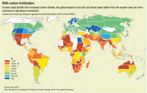
FIGURE 5-7 Impact of increased temperature and precipitation on agricultural productivity. Percentage increases and decreases were calculated assuming additional carbon fertilization. Negative values indicate percentage decreases in productivity. For example, the agricultural productivity in Mexico and the southwestern United States is predicted to decline by 25% or more. SOURCE: Cline 2007. Reprinted with permission; copyright 2008, Peterson Institute for International Economics.
Impacts on Human Health
Theoretical analyses of the health consequences of rising average temperatures and the associated changes in average precipitation have led to research in the following five areas:
-
Heat (and cold)-associated health conditions, including the excess morbidity and mortality attributable to infectious, respiratory, and cardiovascular diseases and to over-exposure that occur after intense or prolonged cold weather and the heat-stress-related morbidity and mortality, especially excess cardiovascular disease mortality after intense or prolonged hot weather. This category could include the potential impacts on occupational health from working in hot and cold climates. These impacts are typically derived by looking at patterns of mortality either by day or season as a function of temperature for major cities and then using regression techniques to estimate temperature associated effects. Investigators differ in choice of daily changes—for example, heat waves, or average seasonal temperatures, the former providing higher estimates but with excess deaths typically limited to more vulnerable subpopulations.
-
Vector-borne diseases, especially malaria (mosquitoes), but also including dengue and yellow fever (mosquitoes), hanta and related viruses (rodents), Lyme and rickettsial diseases (ticks) and bird-borne viruses, such as West Nile and possibly influenza.
-
Sanitation-related disorders, including diarrheal diseases, such as cholera and others that occur with increased frequency in the setting of storms and prolonged droughts.
-
Climate-associated changes in air-pollution health effects, including atmospheric conversion of NOx and hydrocarbons to ozone and of SO2 to its acid forms, which may be related to climate, although climate is not the source of air pollutants.
-
Aeroallergen load associated with altered ecosystems resulting from temperature and rainfall changes. As a consequence, potential increases in rates of upper and lower respiratory track allergies including asthma.
Substantial efforts have been made to model impacts in each category for the United States and other regions of the world based on the study of morbidity and mortality patterns in relation to climate patterns historically.
Accurate prediction of future impacts is substantially limited by the complexity of underlying assumptions about the populations at risk over time. The following factors complicate current efforts to estimate, based on various climate-change scenarios, what the impact on human health will be in the distant future:
-
Demographics and development. All the categories listed above affect different populations differentially, depending on such features as age, underlying health status, and stage of socioeconomic development. For example, the sanitation-related disorders are relevant only in the context of under-development; populations in advanced countries rarely suffer from these impacts under any climate conditions except in a hurricane Katrina-like disaster. Similarly, heat- and cold-associated disorders affect disproportionately the very young and very old, those with chronic health conditions, and those with resource limitations. Any predictions of the impact of a given climate-change scenario demands that explicit assumptions be made regarding the distribution of at-risk people in a given population, introducing more uncertainty.
-
Adaptation. The impact of many purported climate-associated health effects depends on the degree to which the affected population has become adapted to particular conditions. For example, heat-related morbidity and mortality are far more salient in populations living in temperate climates with large seasonal fluctuations in temperature than in those with year-round hot weather because of acclimatization; the rate of change may be a larger determinant than the extent of change in some of these estimates.
-
Technology. Separate from the impact of development on the underlying condition of populations is the potential impact of specific technological changes. For example, a successful malaria vaccine could neutralize the projected impact of increased malaria mortality even in the absence of underlying developmental change in regions of the world with endemic malaria. Likewise, advances in sanitation science and development of new antimicrobial techniques or agents or vector control technologies could substantially alter modeled impacts on sanitation-related effects.
-
Mitigation. Projected effects for each climate-change scenario could be substantially modified by efforts to anticipate the effects and mitigate them. Above and beyond the societal changes anticipated by societal development following its natural path, specific interventions could, in theory, reduce or eliminate effects due to any of the above categories. Interventions could include climate surveillance and institution of remedial steps under conditions of anticipated high risk or introduction of societal countermeasures, such as more stringent air-quality controls or provision of climate-controlled public shelters.
While the importance of each of those factors is widely acknowledged by investigators attempting multisector estimates of the (external) costs of damages related to human health under various scenarios (for example, RICE and DICE and FUND), the cost estimates for damages in each category have been developed generally under the default assumptions that
development and demographic change over time would occur unrelated to intentional efforts to modify or mitigate the impacts of GCC. In other words, it is assumed that technologies and GDP will advance in parallel, and the underlying health status related to development will improve based on projections of regional GDP and global-warming potential, without taking into consideration specific efforts (or their costs) that might specifically offset or modify possible climate-related health effects.
The FUND and the RICE and DICE model estimates for health damages as percentage-lost GDP for the United States and globally reflect two somewhat divergent approaches. Tol (2002a,b) (FUND model), building on previous efforts, approaches the damages for the United States (and also other developed economies) by restricting attention to a single category of effects, namely, “heat-associated health conditions.” FUND incorporates Martens (1998) meta-analysis of data from 17 European and American countries (20 cities)—a model based on seasonal averages—to calculate the impact of temperature under several climate scenarios. None of the other categories of potential health effects is added, possibly resulting in an underestimate. Nordhaus and Boyer (2002) (RICE and DICE), on the other hand, does not use this approach for a U.S. estimate and relies instead on deriving a temperature-associated estimate based on the WHO Global Burden of Disease (Murray and Lopez 1996) estimates for the region, resulting in a very small figure, more than 10-fold lower than the Tol figure.
It is noteworthy that both methods may have underestimated effects attributable to other categories. Most notably on the United States side is the possibility that pollution, interacting with climate, may have greater impact on ozone-related morbidity and mortality than estimates of temperature or pollution separately (for example, Knowlton et al. 2004). Globally, Kjellstrom et al. (2008) published a model that suggests substantial impact of climate in developing countries on the ability to work because of heat stress. The magnitude of this health effect has not been incorporated into either model, nor has either addressed the potential importance of allergy-related disease despite the global epidemic of asthma, still unexplained, already under way. Although Tol offers a range of estimates based on differing assumptions about the composition of the at-risk populations, neither model has tested divergent assumptions about the effects of mitigation, adaptation, or specific technological change.
Other Impacts: Energy Production and Consumption, Socioeconomics, and National Security
Climate change is likely to result in many impacts that are poorly measured or difficult to quantify. In this section, the committee focuses on impacts to industry, population movements, energy supply and consump-
tion, and national security. The greatest risks from climate change are likely to increase instability in vulnerable areas of the world with a consequent potential for increased risk of terrorism and political instability.
Impacts on Energy Production and Consumption
In the United States, global warming will probably lead to modest decreases in heating demand in northern areas and modest increases in cooling demand in the southern area (CCSP 2007). Impacts on energy consumption primarily affect demand for electricity.
The CCSP study showed decreases in energy used in residential, commercial, and industrial space heating as possible effects of climate change. Estimates are quite imprecise. One study (Mansur et al. 2005) found a 2.8% decline in energy use for electricity-only customers, a 2% decline for gas customers, and a 5.7% decline for oil customers corresponding to a 1°C increase in January temperature in 2050. The variation in heating reduction is driven in part by regional variation in heating. Oil accounts for over one-third of heating in the Northeast, whereas electricity-only customers are likely to be located in the South or Southwest. Scott et al. (2005) found a stronger response relative to the results of the CCSP study.
Residential cooling impacts were stronger in the Mansur et al. (2005) study, which found a 4% increase in demand for electricity-only customers for a 1°C increase in July temperature in 2050. Increases for gas and fuel oil customers are 6% and 15%, respectively.
Annual energy consumption is affected by decreased heating and increased cooling costs. Mansur et al. found a 2% increase in residential expenditure and no impact on commercial expenditures at the national level. Others studies have found similar impacts, although regional variation is potentially significant.
Global impacts mirror regional impacts in the United States. Higher latitude regions benefit from reductions in heating, and lower latitude regions face higher costs of cooling (Stern 2007).
Beyond heating and cooling, the CCSP (2007) report found little impact on industrial energy demand (see studies by Amato et al. 2005; Ruth and Lin 2006). Industry may be affected in other ways. In particular, electric outages arising from extreme weather events would have significant impacts on energy-sensitive industries.
Similarly, impacts on energy production are likely to be modest in the aggregate. Regionally, certain areas may experience impacts. Reductions in water in the Northwest could reduce supply of hydroelectricity appreciably. Weather disruptions and extreme events could affect oil and gas supply and refining activities in the Gulf of Mexico. Similar impacts arise globally. Stern (2007, pp. 142-143) reported reductions in nuclear power production
in France during the 2003 European heat wave due to overly warm river water that the plants rely on for cooling.
Socioeconomic Impacts
It is difficult to predict the full range of potential socioeconomic impacts from global climate change. Stern (2007, pp. 128-129) reported that about 7 million people in sub-Saharan Africa have migrated to new regions to obtain food because of environmental stresses on agriculture. In addition to migration, climate change has the potential to create disruptions that affect education and gains in equality of women (Chew and Ramdas 2005). Coastal erosion, rising oceans, and extreme weather all disproportionately affect the most vulnerable members of society. (See a catalog of impacts in Leary et al. (2006).
National Security Impacts
The socioeconomic instabilities described above have implications for national security of the United States, as well as global security. A recent report by the CNA Corporation (CNA 2007) found that climate change will add to instability in already volatile parts of the world (for example, Somalia and Darfur). In addition, the impacts will be felt globally and so create greater strains for the U.S. military as it stretches itself to cover conflicts in various parts of the world (acting either unilaterally or multilaterally).
Population migration will also affect currently stable countries and regions. The United States and Europe, for example, will face increased pressure from immigrant populations. Moreover while underdeveloped regions of the world are disproportionately affected by extreme weather (or are especially vulnerable), stable regions are not immune. The European heat wave of 2003 was estimated to have killed more than 50,000 people (Larsen 2006).
The CNA report highlights especially important regional impacts. Two-thirds of the Arab world currently relies on imported sources of water (CNA 2007, p. 30). Decreased precipitation exacerbates this problem and raises the specter of increased out-migration and land tension with neighbors. Nearly 40% of Asia’s population lives no more than 45 miles from the coast. Sea-level rise could put millions of people at risk for inundation and increased risk of infectious disease (CNA 2007, p. 24).
The military implications of these impacts are twofold. First, U.S. military systems and bases will be stressed. Diego Garcia in the Indian Ocean serves as a major logistics hub for U.S. and British forces in that region of the world. The island at its highest point is only a few feet above sea level (CNA 2007, p. 37). In the event of significant sea-level rise, it may
be possible to adapt by building dikes or other infrastructure but it would come at an economic cost, and the current capabilities of the base may be affected. In addition to impacts on military bases, climate change and severe weather make military missions much more challenging. Extreme weather also creates vulnerabilities for military energy supplies. Electricity systems are subject to outages in extreme weather, and the Department of Defense relies on electricity from the national grid to power critical infrastructure at installations (CNA 2007, p. 38).
A second concern identified by the CNA report is the Arctic. With global warming, retreat of the Arctic ice pack means that the U.S. Navy will have to expand its scope of operations to cover this area. In addition, increased access to the Arctic is likely to bring about increased competition for previously inaccessible resources, including potentially large reserves of oil.
Estimates of Other Impacts
It is extremely difficult to monetize the external costs of political instability, population displacement, national security, and military costs arising from climate change. However, the committee can provide estimates of the external costs arising from increased demand for electricity due to climate change. We briefly discuss below the treatment of these costs in the FUND and DICE models.
The FUND model 3.0 does not provide estimates of most of the socioeconomic costs discussed above, although resettlement costs are included in the costs of sea-level rise. FUND does provide estimates of increased heating and cooling costs based on an equation relating heating (or cooling) to increases in temperature, per capita income, population, and technological improvements. The elasticity of heating with respect to global mean temperature (relative to 1990 levels) is 0.5 for heating and 1.5 for cooling in the FUND base case. The income elasticity of space heating and cooling demand is 0.8 in the base case (Hodgson and Miller 1995, as cited in Downing et al. 1996b). Tol (2009) reported that globally the increased costs of electricity for cooling are the single largest component of the marginal damages from a ton of CO2-eq emissions, while global reductions in heating costs reduce the marginal damages from a ton of CO2-eq emissions.
Nordhaus and Boyer (1999) estimated that a 2.5°C increase in temperature would have negligible costs on energy and modest costs on human settlements ($6 billion in 1990 dollars; see Table 4-11, p. 4-45, of the study). These costs include costs of migration and adaptation as well as losses that occur because of difficulties in responding to sea-level rise or extreme weather. These costs are computed by estimating the capital value of vulnerable areas and assuming a willingness to pay to avoid damages
equal to 1% of the value of at-risk capital (see section Coastal Zone Impact of Climate Change). The authors acknowledged that the method “is at this stage speculative and requires a detailed inventory and valuation of climatically sensitive regions for validation” (pp. 4-21 to 4-22). The authors noted, however, that this topic is likely to be of high impact and cost that will factor in to climate-change policy in important ways.
ECONOMIC DAMAGE FROM IRREVERSIBLE AND ABRUPT CLIMATE CHANGE
The term “abrupt climate change” has several definitions (NRC 2002d; Clarke et al. 2003; Overpeck and Cole 2006). For the purposes of this assessment, a useful definition is articulated by CCSP (2008): “A large-scale change in the climate system that takes place over a few decades or less, that persists (or is anticipated to persist) for at least a few decades, and causes substantial disruptions in human and natural systems.”
By contrast, irreversible climate changes represent fundamental regime shifts in major climatic variables that are likely to persist over hundreds to thousands of years. Irreversibilities are related to abrupt climate changes in that they embody the idea of thresholds or “tipping points” in physical or biogeochemical variables, which once crossed result in a large (implicitly rapid rate) and for all intents and purposes permanent change. In terms of climate responses, changes of this nature include such possibilities as the collapse of the Greenland or West Antarctic ice sheets, loss of coral reefs, or shutdown of the North Atlantic thermohaline circulation. However, incremental climate changes could eventually cross a threshold related to physical processes and thus result in irreversible climate change. One concern about such climate changes is the potential for them to trigger serious or catastrophic follow-on impacts, such as the release of methane and CO2 trapped in ocean sediments and permafrost; loss of biodiversity through extinction, disruption of species’ ecological interactions, and major changes in ecosystem structure; and disturbance regimes, such as wildfire and insects.
Another reflection of this concern is the tendency of these sorts of changes to be discussed in parallel with potential downstream consequences for human society, in particular the value of lost species, ecosystem services, arable land and attendant effects on food security, as well as adverse effects on human settlements, migration, and the potential human insecurity (i.e., refugees, violent conflict) arising therefrom.
An important feature of the preceding definitions is that they say little about the likelihood of occurrence of the events in question. Although it is tempting to view climate thresholds as a bright-line, there is little empirical basis for inferring how much of a change in probability they bring. On one hand, there is the probability of the threshold being reached, which depends
on the trajectory of GHG emissions and consequent radiative forcing. Some indication of the relevant probabilities is given in Table 5-2. On the other hand, how the probability of occurrence of the impacts in question might change for increments in, say, temperatures in excess of the threshold is largely unknown. For example, IPCC (2007a) concluded that 20-30% of assessed species face about a 50% chance of increasingly high risk of extinction as global mean temperatures exceed 2-3°C above preindustrial levels but does not characterize the dependence of the probability of extinction on temperatures beyond the threshold.12 This kind of impact is distinct from events that are low probability but very high consequence. It is unclear whether climate thresholds apply—such as a massive decadal-scale release of methane to the atmosphere from rapid clathrate destabilization.
Solomon et al. (2009) focused attention on atmospheric warming, precipitation changes, and sea-level rise driven by thermal expansion as adverse irreversibilities for which three criteria are met: (1) the relevant changes are already being observed, and there is evidence for their anthropogenic precursors; (2) the phenomena are based on physical principles that are thought to be well-understood; and (3) projections are available and are broadly robust across Earth-system models. These authors use results from a suite of models to construct ranges of long-run equilibrium changes in the climate. Their estimate of the irreversible temperature increase ranges from 1 to 4°C, with a corresponding 0.2-0.6 m sea-level rise per degree of global warming, for an irreversible global average sea-level rise of at least 0.4-1.0 m (and as much as 1.9 m for peak CO2 concentrations in excess of 1,000 ppmv [parts per million by volume]) and complete losses of glaciers and small ice caps adding a further 0.2-0.7 m. The corresponding estimates of shifts in precipitation are subject to considerable uncertainty, but a robust change is an enhanced dry season in several regions (on the order of 20% in northern Africa, southern Europe, and western Australia) and 10% in southwestern North America, eastern South America, and southern Africa for 2°C of global mean warming. The equilibrium dependence of regional dry-season-precipitation impacts on CO2 concentrations is illustrated in Figure 5-8.
At the other end of the spectrum, the implications of these climate changes for biodiversity loss, highly nonlinear impacts—such as ice sheet instability, thermohaline circulation (THC) collapse, and methane clathrate releases—and climate-induced violent conflict represent unknowns that derive from fundamental gaps in scientific understanding of the mechanisms of the relevant impact pathways in Figure 5-1 (NRC 2002d; Tol 2008). For
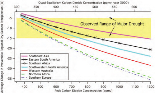
the sake of completeness, brief notes are provided about the current state of the literature in each of these areas.
There are comparatively few quantitative studies of the direct impacts of climate change on ecosystems and biodiversity at broad geographic scales,13 and projecting changes in biodiversity at the regional and global levels is complicated by the need to account for large-scale, potentially non-linear interactions associated with such factors as shifting anthropogenic land use and invasive species (see Sala et al. 2000). The theoretical basis for valuation of ecosystem changes at these scales is very weak. Nicholls et al. (2008) explored a wide range of scenarios of resulting sea-level rise and assessed the impacts of a collapse of the West Antarctic Ice Sheet (WAIS) at 0.5-5 m per century. Their estimates of annual costs, which are not explicitly linked to temperature change, ranged from $0-28 billion in 2050 to $0.1-31 billion in 2100.
The full range of impacts arising from a slowdown or collapse of the Atlantic THC has yet to be systematically characterized. The only studies from which cost figures can be drawn are Keller et al. (2004), who arbitrarily assumed an uncertain cost in the range of 0-3% of gross world product, and Link and Tol (2004), who estimated that THC shutdown increases the marginal damage of GHG emissions by $0.1-2.2 per ton of carbon. The seemingly small magnitude of these figures may be appreciated when one considers that, in the Link and Tol study, THC collapse has a negligible influence on global average surface temperature but has a substantial impact on temperatures in the United States, Canada, and western Europe, inducing cooling of 0.5-1.5°C by 2150 and 1-3°C by 2300.
Considerable scientific uncertainty still besets the characterization of methane releases from clathrates in ocean sediments and permafrost. The most widely cited study by Harvey and Huang (1995) estimates a cumulative methane release of 53-887 gigatonnes of carbon after 2,000 years (see Table 9), resulting in an equilibrium atmospheric temperature rise of 1-9°C (see Figure 9). These authors find an amplification of global warming of 10-25%, but this range depends strongly on assumptions about the climate sensitivity and the warming due to projected anthropogenic CO2 emis-
sions, and is substantially outweighed by the latter uncertainties. Results by Renssen et al. (2004) highlight the importance of uncertainties regarding the “worst case” quantity of methane released. A massive emission (1,500 GtC) over the course of a millennium would entail large climate changes,14 having peak additional surface warming of 2.6°C on average and up to 10°C at the poles, accompanied by regime shifts in the global overturning ocean circulation.
The discussion above describes the possibility of extreme climate changes that could result in large, irreversible economic damages to the planet. As noted at the beginning of the chapter, the possibility of extreme events is not handled well by IAMs in calculating the marginal damages of CO2. The RICE and DICE models attempt to handle extreme events by calculating what a risk-averse individual would pay to avoid a catastrophic event (of given probability) that would reduce GDP from 22% to 44%, depending on the region of the world. The probability of such an event is calculated, for each T, on the basis of expert judgment. For a 2.5°C change in mean global temperature, willingness to pay to avoid catastrophic risk ranges from 1.9% of GDP in OECD-Europe and India to 0.45% of GDP in the United States. The corresponding figures are 10.79% and 2.53% of GDP to avoid catastrophic risk associated with a 6°C change in mean global temperature.
Weitzman (2009) demonstrated that, if one were to ask a risk-averse individual what he would pay to avoid the gamble described above, the amount would be infinite if the distribution over the catastrophic GDP loss were “fat-tailed” (formally, if the distribution has an infinite moment generating function). Clearly, the nature of the probability distribution of catastrophic outcomes matters and is handled only imperfectly by the willingness to pay calculations described in the preceding paragraph or by the Monte Carlo simulations performed to capture uncertainty in the key parameters of IAMs. The key problem here is that low-probability extreme-impact events located in the fat tails, which are extremely difficult to quantify, might drive the results of cost-benefit analysis. This possibility is disturbing because the answers to important questions about how much effort to put into climate-change mitigation can depend to an uncomfortable degree on subjective estimates about the likelihood of catastrophic outcomes.
AGGREGATE IMPACTS OF CLIMATE CHANGE
To quantify the marginal impact of an additional ton of GHG emissions requires a number of steps beyond quantifying the individual impacts associated with a particular magnitude of climate change. Within each region, for a particular climate-change scenario (for example, doubling of CO2 concentrations in the atmosphere), individual components of impact must be aggregated across sectors, raising difficulties for inclusion of impacts that have not been expressed in monetary metrics and interactive effects, such as that between water and agriculture. Next, because the impacts of GHG emissions emitted anywhere are felt globally, there is much interest in understanding the global impacts of climate change, not simply the effects of each country’s emissions within its own borders. This factor requires aggregating impacts on people with widely differing incomes, raising questions about whether monetized impacts should be adjusted to account for differing marginal values of income across countries. Moreover, because the consequences of current GHG emissions are expected to persist for centuries, it is necessary to aggregate impacts on people living at different times in the future. Previous surveys of these issues include Pearce et al. (1996), Tol and Fankhauser (1998), Tol et al. (2000), Smith et al. (2001), Hitz and Smith (2004), Stern (2007), Yohe et al. (2007), and Tol (2008).
Tol (2008) identified 13 published studies that have estimated the monetized impacts of climate change at a global level; several of them also include total climate-change damage estimates individually for the United States and other regions (Fankhauser 1995a; Tol 1995, 2002b; Nordhaus 1994a,b, 2006; Nordhaus and Yang 1996; Plambeck and Hope 1996; Mendlesohn et al. 2000a,b; Nordhaus and Boyer 2000; Maddison 2003; Rehdanz and Maddison 2005; Hope 2006). In addition, the Nordhaus (2008) study contains an update based on Nordhaus and Boyer (2000), and at least another four published studies contain total-damage estimates for the United States alone (Nordhaus 1991; Cline 1992; Titus 1992; Mendelsohn and Neumann 1999). These estimates are not independent because many of them represent revised estimates by the same researchers over time (for example, Nordhaus, Tol, Hope, and Maddison), and other estimates are based on models that draw from several other prior studies (for example, impact valuation in Plambeck and Hope (1996) derives from Tol (1995) and Fankhauser (1995b); see discussion in Tol (2008). A review of impact estimates within IAMs (Warren et al. 2006b)—including the DICE and RICE models (Nordhaus), FUND model (Tol), and PAGE model (Hope)—found that the impacts in these models are based on literature from 2000 and earlier.
Table 5-7 summarizes results from many of these studies, for consistency expressed in terms of percentage loss in GDP. Most, but not all of the
TABLE 5-7 Estimates of Total Damage Due to Climate Change from Benchmark Warming (Percentage Change in Annual GDP)
|
Study |
Temperature Change (°C) |
Globale |
United States |
Range Across Regions |
|
2.5-3.0°C warming benchmark |
|
|
|
|
|
Nordhaus (1991) |
3.0 |
NA |
−1.0 |
NA |
|
Cline (1992) |
2.5 |
NA |
−1.1 |
NA |
|
Nordhaus (1994a) |
3.0 |
−1.3 |
NA |
NA |
|
Nordhaus (1994b) |
3.0 |
−1.9c |
NA |
NA |
|
Fankhauser (1995b) |
2.5 |
−1.4 |
−1.3 |
−4.7-−0.7 |
|
Tol (1995) |
2.5 |
−1.0 |
−1.0 |
−8.7-0.3 |
|
Nordhaus and Yang (1996) |
2.5 |
−1.7a |
−1.1 |
−2.1-0.9 |
|
Plambeck and Hope (1996) |
2.5 |
−2.5a |
−1.6 |
−8.6-0.0 |
|
Nordhaus and Boyer (2000) |
2.5 |
−1.5 |
−0.5 |
−4.9-0.7 |
|
2.5 |
0.00.1 |
NA |
||
|
Hope (2006)d |
2.5 |
−1.0 |
−0.3 |
−3.1–0.3 |
|
Nordhaus (2006)b |
3.0 |
−1.0 |
NA |
NA |
|
Nordhaus (2008) |
2.5 |
−1.8 |
−0.7 |
−20.0–16.4 |
|
Other warming benchmarks |
|
|
|
|
|
Titus (1992) |
4.0 |
NA |
−2.5 |
NA |
|
Tol (2002b) |
1.0 |
2.3 |
3.4 |
−4.1–3.7 |
|
NOTES: Positive damage estimates indicate benefits from warming. NA indicates data are not available. aAs computed by Tol (2008). bEstimate includes only market impacts; nonmarket impacts are not monetized. cMedian estimate from an expert opinion survey of 19 individuals. dThe study’s mean estimates are given. eGlobal GDP losses are simple (unweighted) sums of regional GDP losses. |
||||
scenarios are benchmarked to a 2.5-3°C temperature increase by 2100 associated with central estimates of the likely warming from a doubling of GHG concentrations in the atmosphere. Note that Mendlesohn et al. (2000a,b) and Nordhaus (2006) include only market impacts, while the other studies also include estimates of nonmarket impacts, at least to some degree.15
Table 5-7 shows that these studies typically estimate the aggregate global market plus nonmarket impact of doubling GHG concentrations at 1-2% of lost world GDP. The aggregate impacts mask significant differences in regional impacts and in the underlying impacts for individual damage
categories estimated within each study. Estimated percentage damages tend to be lower in industrialized countries but significantly higher in many developing countries with relatively higher current temperatures, heavier dependence on agriculture, and lower adaptive capacity. No individual impact category consistently dominates other categories across studies. Previous surveys have also been careful to note the low quality of the numbers and the many shortcomings of the underlying studies.
In addition to differences across aggregate climate-impact studies in terms of methods and estimated regional and individual impact categories, there are a number of other key assumptions and sensitivities. One issue is whether GDP impacts in individual regions are weighted during aggregation to a global total. The global estimates noted above simply add up the estimated regional impacts in dollar terms (that is, they are output weighted) regardless of income levels in the different regions. However, it is widely accepted that individuals with low income tend to value a given dollar impact more heavily than a relatively high-income individual. This factor is known as the declining marginal utility of income, and approaches for incorporating it are often called “equity weighting” or “population weighting” (if global losses are based on regional percentage losses weighted by population shares as opposed to output shares). Estimates that allow for equity weighting typically find significantly more negative aggregate global impacts because regions with more substantial projected impacts are also relatively poor (Yohe et al. 2007).
Estimates of total climate damage also depend critically on the degree of temperature change that is being assessed. With the exception of the Titus (1992) and Tol (2002b) assessments of a 4°C and 1°C temperature increase, respectively, all the other studies in Table 5-8 focus on a benchmark warming scenario of 2.5-3.0°C, corresponding to best estimates of eventual temperature change from a doubling of GHG concentrations. Unsurprisingly, the pattern among available studies is that—beyond some amount of warming that is beneficial for certain regions and impact categories—greater degrees of temperature increase are associated with correspondingly higher damages.16
As an approximation, modeling assessments (for example, using DICE and RICE, FUND, and PAGE) that explore a range of emission, concentration, and temperature scenarios tend to assume that damages are proportional to the size of the world economy and that the fraction of world GDP lost (total or per capita) is a power function of temperature increase. The power function is calibrated to the damage estimate from benchmark
|
16 |
Several studies have found positive impacts of climate change on agriculture in Canada, Europe, and parts of China (see Figure 5-7 from Cline [2007]). Heating requirements are also predicted to decline in Russia and parts of Europe. |
TABLE 5-8 Marginal Global Damages from GHG Emissions: Estimates from Widely Used Models
|
Model |
Study |
Marginal GHG Damage ($/ton CO2) |
Discount Rate (%)a |
Climate-Warming Scenario |
Total Global Climate Damage (% GDP) |
|
DICE |
Nordhaus (2008) |
8e 8 |
~4.5 |
No control: 3.1°C in 2100; 5.3°C in 2200 Optimal: 2.6°C in 2100; 3.5°C in 2200 |
−1.8% at 2.5°C −4.5% at 4.0°C −7.1% at 5.0°C −10.2% at 6.0°C |
|
FUND |
Tol (2005a)d |
0 2 6 |
5 3 2 |
No control: 3.7°C in 2100; 6.7°C in 2200 |
~0% at 2.5°C ~ −1% at 4.0°C ~ −1% at 5.0°C |
|
PAGEb |
Hope (2006)c Hope and Newbery (2008) |
6 (1-17) 22 (4-60) 108 (21-284) |
~4.5 ~3 ~1.5 |
No control: 4.1°C in 2100; 7.9°C in 2200 |
−1.0% at 2.5°C −2.6% at 3.9°C −11.3% at 7.4°C |
|
|
Stern (2007) |
102 36 |
1.4 |
No control: 3.9°C in 2100; 7.4°C in 2200 Stabilize at 550 ppm CO2-eq: eventual 3°C |
−1.0% at 2.5°C −2.6% at 3.9°C −11.3% at 7.4°C |
|
NOTE: Negative numbers indicate a negative impact on GDP. aDiscount rate changes over time in Nordhaus (2008) and Hope (2006); the approximate effective discount rate is given. bFor PAGE model, mean global GDP impacts are given in Dietz et al. (2007), including market, nonmarket, and risk of catastrophic impacts. cMean estimate for 2001 emissions with 5th-95th percentile confidence interval from uncertainty analysis in parentheses. dEstimate is for emissions in 2000 from FUND version 2.4. eEstimate is for emissions in 2005. |
|||||
warming (that is, it is one point on the function) and an assumed temperature level corresponding to zero damages. A linear relationship (that is, percentage of climate damages per degree temperature change is constant) corresponds to a power of 1, and a quadratic or cubic relationship corresponds to a damage exponent of 2 or 3. The DICE model (Nordhaus 2008), for example, assumes a quadratic damage function based on Nordhaus and Boyer (2000), yielding estimates of global climate damages increasing over fourfold from −1.8% to −8.2% of world GDP for a twofold increas in temperature from 3°C to 6°C. The PAGE model (Hope 2006), on the other hand, allows for a damage exponent ranging from 1 to 3, with an
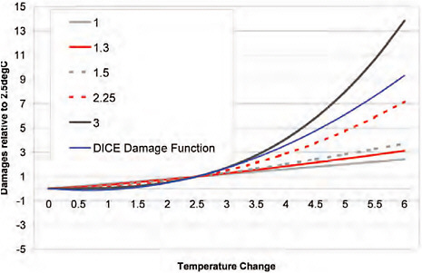
FIGURE 5-9 Dependence of GHG damage on the amount of temperature change. The lines show the PAGE 2002 damages for damage exponents between 1 and 3. The damage function of the DICE model is also shown for comparison. In this figure, positive values indicate economic losses, and negative values indicate benefits from warming. SOURCE: Stern 2007, Technical Appendix.
associated range of global impact that varies by a factor of almost 6 for a 6°C temperature increase (see Figure 5-9, where the PAGE damage function for 6°C is about 2.4 times the level at 2.5°C for linear damages, while it is about 14 times as high assuming cubic damages).
Yet, in the absence of substantial mitigation action, projections of baseline GHG emissions tend to imply estimates of likely temperature increase that are significantly greater than that associated with a doubling of GHG concentrations. For example, the IPCC (2007a, p. 180, Figure 5.1) referenced plausible projections of GHG concentrations that go near to and beyond 1,000 ppm by 2100, with an associated best estimate global mean temperature increase above preindustrial levels of about 5-6°C and a likely range from just under 4°C to over 8°C. However, little is known about the precise shape of the temperature-damage relationship at such high temperatures.17 Figure 5-10 illustrates the dependence of GHG damage, as a percentage of global GDP, on the amount of temperature change.
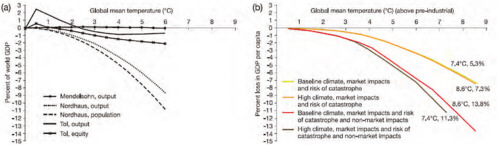
FIGURE 5-10 Dependence of greenhouse gas (GHG) damage, as a percentage of global gross domestic product (GDP), on the amount of temperature change. (a) Damage estimates represented as a percentage of global GDP, as a function of increases in global mean temperature. (b) Damage estimates, as a percentage of global GDP per capita, are correlated with increases in global mean temperature. In this figure, positive values indicate benefits from warming. SOURCE: IPCC 2001, p. 1032 and Stern 2007 (as cited in Yohe et al. (2007, p. 822).
MARGINAL IMPACTS OF GREENHOUSE GAS EMISSIONS
Given an estimate of the monetized global impact of a particular climate-change scenario at a particular future point in time, this total-damage estimate can then be translated into a marginal damage per ton estimate (often called the “social cost of carbon”) by evaluating the linkage between current GHG emissions and future climate-change impacts (see Equation 5-2). It is usually estimated as the net present value of the impact over the next 100 years (or longer) of 1 additional ton of CO2-eq emitted into the atmosphere. It is this marginal damage per ton of emissions that is normally used as a measure of the global climate externality. This measure requires assumptions about the emissions-temperature and temperature-damages linkages over time, as well as the rate at which future damages are discounted back to the present to account for differing valuation of monetary impacts felt at different points in time. Finally, uncertainties at each step of the analysis imply that different possible future conditions may yield widely differing impacts. The expected value of damages may be more sensitive to the possibility of low-probability catastrophic events than to the most likely or best-estimate values.
There have been many previous reviews of existing estimates of the marginal damages from GHGs, including Pearce et al. (1996), Tol (1999, 2005b, 2008), Clarkson and Deyes (2002), and Yohe et al. (2007). Tol (2008) identifies 211 marginal-damage estimates from 50 studies, although this number does not imply we know more about marginal than total damages (there are only 12 global total-damage estimates, as shown in Table 5-7). The explanation for how so many marginal costs can be generated from so few total-damage estimates lies in the variety of additional modeling assumptions that must be incorporated to translate total into marginal damages. As alluded to above, in addition to the benchmark estimate of total damages, important other assumptions include the change in damages with increased warming and with growth and changes in the composition of economic activity over time, the assumed emissions scenario, the climate sensitivity to GHG concentrations, the rate used to discount future impacts to the present, the timeframe over which impacts are considered, and the treatment of uncertainty and risk aversion. Box 5-2 discusses approaches used to determine a discount rate.
Pearce et al. (1996, p. 215, Table 6.11) summarized early estimates of marginal GHG damages, which ranged from $3 to $62 per ton of CO2-eq for emissions occurring in the 2001-2010 decade.18 As part of a United Kingdom effort to assess the social cost of carbon, Clarkson and Deyes (2002) suggested a pragmatic approach could be to use a central
estimate of $35 per ton of CO2-eq, along with a sensitivity range of half and double this amount ($17-70 per ton of CO2-eq). Tol (2005b) identified 103 marginal-climate-damage estimates from 28 published studies, finding a median estimate of $4 per ton CO2, a mean of $25 per ton CO2, and a 95th percentile of $96 per ton CO2-eq across the estimates. Tol (2005b) also found that the subset of studies published in peer-reviewed journals reported lower estimates on average, with a mean of $12 per ton CO2-eq. (The Tol [2005b, 2008] values are not adjusted for inflation.) Summarizing 211 estimates identified in Tol (2008) yields a median estimate of $8 per ton CO2-eq, a mean of $29 per ton CO2-eq, a 5th and 95th percentile of $0 and $105 per ton CO2-eq, respectively, and a peer-reviewed mean of $14 per ton CO2-eq (University of Hamburg 2009). In cases where a single study generated multiple estimates, Tol (2008) included a relative weight for each estimate that was provided by the author of each study. Using these weights, one can construct a single weighted estimate for each of the 50 studies. Summarizing these 50 estimates from individual studies yields a median estimate of $10 per ton CO2eq, a mean of $30 per ton CO2-eq, and a 5th and 95th percentile of $1 and $85 per ton CO2-eq, respectively. Note, however, that due to the lack of necessary information, Tol did not adjust individual estimates for inflation, nor did he account for the timing of emissions (that is, the year they occur) or the GHG concentration and temperature scenario onto which those emissions are added. Adjusting for inflation from the study year to current dollars would make these figures higher. The underlying estimates also differ in terms of their assumed discount rates and how they aggregate regional impacts (using output, equity, or population weighting), among other factors.
To provide a more consistent comparison of marginal-damage estimates, it is helpful to focus on estimates using the most widely used impact assessment models, DICE, FUND, and PAGE, as shown in Table 5-9. The estimates represent the marginal damages from current emissions against an assumed reference case climate scenario without GHG mitigation. This subset of estimates spans approximately the same range as discussed above, from roughly 0 to $100 per ton of CO2-eq. The table demonstrates that virtually all of the variation can be understood as a function of differences across the studies in what is assumed about the discount rate and the magnitude of GDP losses expected from uncontrolled warming. Nordhaus and Yang (1996) made the same point, noting that “the two crucial parameters are the discount rate (which indicates the relative importance of the future compared to the present) and the damages from climate change (which measure the willingness to pay to prevent or slow climate change). It is interesting to note that both major uncertainties involve human preferences rather than pure questions of ‘fact’ about the natural sciences” (emphasis in original).
|
BOX 5-2 Discounting and Equity Weighting Quantifying the damages from GHG emissions requires aggregation of damages that occur at different times extending centuries into the future and to different populations across the globe at each point in time. The method chosen for aggregation has implications for how effects on different people are weighed. Two methods for aggregating effects on different people are common: using monetary and utility measures. The monetary measure assumes that $1 of benefit to one person is equally as good as $1 of benefit to another. The utility measure assumes that the gain in utility (or well-being) from receiving $1 is larger for a poor person than a rich person because the poor person is likely to have more pressing needs. Aggregating across people using the monetary measure is straightforward: One simply sums the monetary values of benefits and harms across the relevant population. To implement the utility-based approach, one needs to make some assumptions about how individual utility varies with income (or wealth). Often, it is assumed that utility is proportional to the logarithm of income or to a power function of income, where the power is less than 1. These functions have the property that utility increases with income but at a diminishing rate. After choosing a function, one can weight the monetary value of benefits and harms to each person by the incremental utility of income and sum these values. This “equity weighting” gives more weight to the same monetary value of damages when they are suffered by a poor person rather than a rich person. For aggregating effects across time, it is conventional to discount the monetary value of future effects by a factor of [1/(1 + r)]t that depends on the discount rate r and number of years in the future t at which the effect occurs. The present value of a stream of effects occurring at various times in the future is calculated by summing the discounted monetary values of the effects. In determining the appropriate discount rate to use for aggregating effects on the current and some future generation, one can distinguish between descriptive and prescriptive ap |
|
proaches. The descriptive approach infers the rate at which society chooses between consumption at different times from market interest rates. In contrast, the prescriptive approach derives the appropriate discount rate on monetary values (the consumption discount rate) as the sum of utility and growth discount rates. The utility discount rate is the rate at which the future generation’s utility is discounted relative to the present generation’s. Many scholars have suggested that it is inappropriate to value other people’s well-being less simply because they come later in time and so argueed for a utility discount rate of zero. The growth discount rate accounts for differences in income between the current and future generation. If the future generation will have greater income than the current generation, it will lose less utility from $1 of damages than the current generation will. To aggregate the effects on utility, it is necessary to down-weight the monetary value of the damages to the future generation, just as one would down-weight the monetary value of effects on rich people at the same point in time in accordance with equity weighting. The extent of this growth discounting effect depends on the economic growth rate (that determines the difference in income between the two generations) and the utility function (that determines how much the incremental effect of income on utility falls). If the future generation is poorer than the present, the growth discounting effect will apply in the opposite direction and will give greater weight to the monetary value of damages suffered by the future generation. Following the prescriptive approach, Stern (2007) adopt a near-zero utility discount rate of 0.1% per year, a relatively small value of the rate at which the incremental effect of income on utility falls to 1 (corresponding to a logarithmic utility function), and a low rate of economic growth, 1.3% per year. Together, these yield a consumption discount rate of 1.4%. In contrast, Weitzman (2007a,b) suggests that more plausible values are roughly 2%, 2, and 2%, yielding a much larger consumption discount rate of 6%. Nordhaus (2008) uses the descriptive approach; he calibrates his model parameters so that the consumption discount rate is consistent with market interest rates, yielding a discount rate of 4.5%. |
Perhaps the clearest illustration of the influence of the discount rate is a comparison of the “no-control” relatively high (4.5%) discount rate scenario of Hope (2006) and the low discount rate (1.4%) of Stern (2007), which yield marginal damage estimates of $6 and $102 per ton, respectively: a 17-fold difference. Both studies used the same version of the PAGE model, so the only significant difference in assumptions is the discount rate. When Hope and Newbery (2008) applied approximately the same discount rate as Stern (2007) to the PAGE model, they found a similar marginal-damage estimate of $108 per ton CO2. Similarly, the Nordhaus (2008)
estimate of $8 per ton CO2, which also used a relatively high discount rate of about 4.5%, is quite close to the estimate of Hope (2006) using a 4.5% discount rate. Finally, when Nordhaus (2008) applied low discount rates similar to Stern’s to the DICE model, he found a marginal-damage estimate similar in magnitude to Stern’s ($88 per ton CO2-eq).
The rate at which future damages from current emissions are converted to present values in Stern (2007) is only slightly greater than the rate at which damages for an incremental increase in global temperature are projected to grow over time. In Stern (2007), damages are a fraction of world GDP per capita that depends on climate change. The rate at which GDP per capita is assumed to grow (1.3% per year) is nearly as large as the discount rate (1.4% per year). With impacts rising almost as fast as they are being discounted, it is primarily the limited time horizon (2200 in the PAGE model) that constrains the marginal-damage estimate from becoming virtually unbounded, given that the effects of current emissions on climate will persist for centuries. In contrast, the discount rates assumed in Nordhaus (2008) and Hope (2006) are high enough that even after accounting for these additional growth effects the present value of damages in the distant future is low.
The growth in incremental damages over time underpins the rationale for a marginal (per ton) GHG damage that rises over time. For example, in the PAGE model, marginal damages rise by about 2.4% per year (Hope and Newbery 2008), and in the DICE model, marginal damages rise by about 2.0% per year (Nordhaus 2008). Over a 20-year period (for example, from 2010 to 2030), marginal damages rising at a rate of 2-3% per year would increase in total by a factor of 50-80%. This estimate is due to a combination of a larger economy being affected and increasing proportionate impacts of increasing temperatures (that is, nonlinearity of the damage function).
The marginal damages from current emissions do not decrease appreciably for alternative scenarios with significantly lower GHG emissions and temperature increases in Nordhaus (2008) or in Hope and Newbery (2008). According to Hope and Newbery (2008), this finding is due to convexity of the damage function being roughly offset by concavity in the concentration-temperature relationship, which is logarithmic. Given that Stern also uses the PAGE model, it is surprising that Stern (2007) found that marginal damages fall dramatically from $102 per ton under a no-control scenario to $36 per ton CO2-eq under a 550-ppm stabilization scenario. Although Stern (2007) does not provide an explanation for the derivation of these results, it appears to be a result of the much lower discount rate assumed in Stern, which gives higher weight to future damages and which are much lower in a stabilization than no-control scenario. In contrast, Nordhaus (2008) and Hope (2006) used significantly higher discount rates
where these future damages (or lack thereof) matter less. One implication is that even low discount rate scenarios that give rise to high marginal damages with no climate mitigation may be consistent with substantially lower marginal-damage estimates (and corresponding Pigouvian emission prices) if, in fact, controls are undertaken. Put differently, even if one accepts marginal-damage estimates on the order of $100 per ton, the implication is not that emission prices at this level would be efficient.
At the other end of the range in Table 5-8 are the estimates from the FUND model. These estimates also demonstrate the importance of the discount rate for present value marginal GHG damages, implying that GHG emissions move from having negligible effects (and in some scenarios positive benefits) with relatively high discounting of 5%, to a larger impact of $6 per ton CO2-eq with relatively low discounting of 2%. The generally lower estimates of FUND are clearly due to the assumed damage function, which specifies benefits to global GDP up until about a 2-2.5°C of warming. Even after this point, damages do not go much beyond about 1% of lost GDP even for large temperature increases, in contrast to the other models where damages increase nonlinearly.
The marginal damages of GHG emissions may be highly sensitive to the possibility of catastrophic events. Although a number of potentially catastrophic outcomes have been identified (for example, release of methane from permafrost that could rapidly accelerate warming, collapse of the West Antarctic or Greenland ice sheets raising sea level by several meters, and changes in North Atlantic currents that would dramatically alter European climate), the damages associated with these events and their probabilities are very poorly understood. Nordhaus and Boyer (2000) and Stern (2007) included some provision for catastrophic outcomes that could result in the loss of perhaps one-quarter of world GDP. Weitzman (2009) raised the even more sobering possibility that the probabilities of extreme outcomes are much larger than currently estimated. If taken into account, low-probability extreme outcomes, such as the possibility of a 10° or even 20°C increase in global mean temperature that could virtually destroy civilization as we know it, could dominate the expected value of damages, making it much greater than the values described above.19
Given the uncertainties and the still preliminary nature of the climate-damage literature, the committee finds that only rough order-of-magnitude estimates of marginal climate damages are possible at this time. Depending on the extent of future damages and the discount rate used for weighting future damages, the range of estimates of marginal global damages can vary by two orders of magnitude, from a negligible value of about $1 per ton to $100 per ton of CO2-eq. Roughly an order of magnitude in difference
can be attributed to discounting assumptions, and another to assumptions about future damages from current emissions. Table 5-9 summarizes these findings for discount rates of 1.5%, 3.0%, and 4.5%, respectively, and for relatively low and higher climate-damage assumptions (corresponding roughly to FUND-level damages versus DICE- or PAGE-level damages). For a discount rate of about 3%—a typical rate for use in long-term environmental analysis in the United States and elsewhere—the comparable marginal-damage estimates could be on the order of about $3 per ton to $30 per ton CO2-eq for relatively low versus higher damage assumptions.20 As discussed earlier, however, the damage estimates at the higher end of the range are associated only with emission paths without significant GHG controls. Therefore, care must be taken in translating these estimates for use in policies for decreasing GHG emissions. In Stern (2007), for example, the marginal-damage estimate is $36 per ton CO2-eq for a stabilization trajectory associated with stabilization at about 550 ppm CO2-eq, not the $102 per ton Stern found associated with uncontrolled emissions.
As described above, marginal-damage estimates for emissions in 2030 could be as much as 50-80% larger than those estimates. Estimates of the damages specifically to the United States would be a fraction of those levels because the United States is only about one-quarter of the world’s economy, and the proportionate impacts on the United States are generally thought to be lower than for the world as a whole (see Table 5-7).
Table 5-10 presents three different estimates of external global damages from GHG emissions on a per unit basis. The damages were calculated by multiplying GHG emission rates from Chapters 2 (electricity), 3 (transportation), and 4 (heat) by each of the committee’s assumed low, middle, and high marginal damages of $10, $30, and $100 per ton CO2-eq.
In conclusion, the committee finds that the relative weight placed on potential impacts occurring decades to centuries in the future is absolutely central to the determination of a present value measure of the damages from current GHG emissions. Over these time horizons, the discount rate carries with it implications for intergenerational distribution. As with any social analysis involving significant distributional impacts, it is therefore
TABLE 5-10 Illustration of Ranges of Climate-Related Damages for Selected Categories of Energy Use in the United States, 2005
|
Sector |
Fuel and Technology |
Climate-Related Damages for $10-30-100/Ton CO2-eqa |
|
Electricity |
|
|
|
|
Coal plants (biomass)b |
1-3.0-10 ¢/kWh |
|
|
Natural gas plants |
0.5-1.5-5 ¢/kWh |
|
|
Nuclear, wind, solar |
Much lower than natural gas |
|
Transportation |
|
|
|
|
Cellulosic E85/car |
0.02-(0.15-0.25)-2 ¢/VMT |
|
|
CNG |
0.04-0.4-4.0 ¢/VMT |
|
|
Gasoline hybrid |
0.04-0.4-4.0 ¢/VMT |
|
|
Gasoline/car |
0.06-0.6-6.0 ¢/VMT |
|
|
E10 |
0.06-0.6-6.0 ¢/VMT |
|
|
H2(g) |
0.03-0.3-3.0 ¢/VMT |
|
|
Diesel/car |
0.05-0.5-5.0 ¢/VMT |
|
|
E85 corn/car |
0.05-0.5-5.0 ¢/VMT |
|
|
Grid-dependent HEV or EVc |
0.05-0.5-5.0 ¢/VMT |
|
Building and Industrial for Heating |
|
|
|
|
Natural gas combustiond |
0.07-0.7-7.0 $/MCF |
|
aRounded to one digit, 2007 USD. bBiomass can be co-fired with coal in quantities up to about 20%. cRanges based on use of the fuel in a representative group of vehicles. Grid-electric cars are usually smaller than fleet average cars, so their better performance per vehicle mile traveled (VMT) is also dependent on use of smaller cars with lesser driving ranges. dFuture additions to supplies may include imported liquified natural gas, which will include nonclimate damages outside the United States at the source and will have increased climate damages in the range of 30% or more depending on the gas field and the liquefaction plant details. ABBREVIATIONS: CNG = compressed natural gas; HEV = hybrid electric vehicle: EV = electric vehicle; MCF = thousand cubic feet. |
||
crucial for decision makers not only to look at singular summary statistics (such as present value marginal damages) but also to understand the magnitude of impacts as individuals will bear them, both across time and at different points in time across regions. This concern is not particular to climate change, but the very long time frames associated with GHG residence in the atmosphere and with thermal inertia of the oceans raise the issue of discounting to a level that is present in few other problems. Nonetheless, the committee also finds that a consistent framework for discounting impacts occurring over similar time frames across all potential policy investments is essential for reasoned policy analysis.
RESEARCH RECOMMENDATIONS
The committee makes the following recommendations to improve the understanding of physical, biological, and human impacts, as well as economic valuation aspects related to climate change.
-
More research on climate damages is needed, as current valuation literature relies heavily on climate-change impact data from the year 2000 and earlier (see Tol [2008] for a number of fruitful areas).
-
Marginal damages of GHG emissions may be highly sensitive to the possibility of catastrophic events. More research is needed on their impacts, the magnitude of the damage in economic terms, and the probabilities associated with various types of catastrophic events and impacts.
-
Estimates of the marginal damage of a ton of CO2 include aggregate damages across countries according to GDP, thus giving less weight to the damages borne by low-income countries. These aggregate estimates should be supplemented by distributional measures that describe how the burden of climate change varies among countries.


