E
Comparison of Fuel Consumption and Fuel Economy
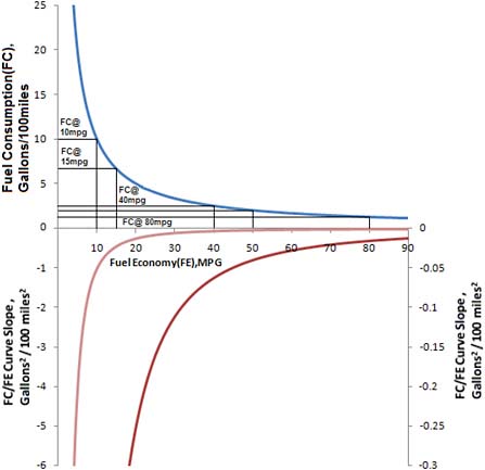
Figure E.1 shows the relationship between fuel consumption (FC) and fuel economy (FE), including the slope of the curve that relates them (Johnson, 2009). The slope, which is negative, and the shape of this relationship are important. The slope indicates the change in FC relative to a change in FE—e.g., when the magnitude of the slope is high, such as at 10 mpg, there is large change in FC for a small change in FE. At 50 mpg, however, there is little change in FE since the magnitude of the slope is very low and approaching zero as indicated by the right-hand slope scale on Figure E.1. Fuel consumption decreases slowly after 40 mpg since the slope (lower curve and right-hand scale) of the fuel consumption versus fuel economy (Figure E.1) curve approaches zero. The slope rapidly decreases past 40 mpg since it varies as the inverse of the FE squared, which then results in a small decrease in FC for large FE increases. This fact is very important since fuel consumption is the metric in CAFE. Furthermore, the harmonic average1 in the CAFE standards is determined as the sales-weighted average of the fuel consumption for the urban and highway schedules converted into fuel economy. Figure 2.2 was derived from Figures 2.1 and E.1 to show how the share of fuel consumption decrease is related to percent increase of fuel economy.2 The curve in Figure 2.2 is independent of the value of fuel economy and is calculated by the equation in footnote 2. For example, the fuel consumption is 2.5 gal/100 mi at 40 mpg and 1.25 gal/100 mi at 80 mpg, which is a 40 mpg change in fuel economy (100 percent increase in FE) and a change in fuel consumption of only 1.25 gal/100 mi (50 percent decrease in FC), as shown by the lines on the FC vs. FE curve in Figure E.1. In going from 15 to 19 mpg, there is an approximate 1.25 gal/100 mile change in fuel consumption. The nonlinear relationship between fuel consumption and fuel economy gives significantly more weight to lower fuel economy vehicles (15-40 mpg—i.e., 6.5-2.5 gal/100 mi) than to those greater than 40 mpg. Going beyond 40 mpg there is a perception that fuel efficiency is improving faster than the actual change in fuel consumption. For a fleet that contains a large number of vehicles in the 15-35 mpg range, the vehicles with a fuel economy greater than 40 mpg contribute only a small amount to the weighted average CAFE fuel economy, assuming that there are fewer 40-mpg vehicles than 15- to 35-mpg vehicles.
Fuel consumption difference is also the metric that determines the yearly fuel savings in going from a given fuel economy vehicle to a higher fuel economy vehicle:
(E.1)
where FC1 = fuel consumption of existing vehicle, gal/100 mi, and FC2 = fuel consumption of new vehicle, gal/100 mi. The amount of fuel saved in going from 14 to 16 mpg for 12,000 miles per year is 107 gal. This savings is the same as a change in fuel economy for another vehicle in going from 35 to 50.8 mpg. Equation E.1 and this example again show how important fuel consumption is to judging yearly fuel savings.
REFERENCE
Johnson, J. 2009. Fuel consumption and fuel economy. Presentation to the National Research Council Committee to Assess Fuel Economy Technologies for Medium- and Heavy-Duty Vehicles, April 7, Dearborn, Mich.
|
1 |
Harmonic average weighted |
|
2 |
If FEf = (FE2 − FE1)/FE1 and FCf = (FC1 − FC2)/FC2 where FE1 and FC1 = FE and FC for vehicle baseline and FE2 and FC2 = FE and FC for vehicle with advanced technology, then, FCf = FEf /(FEf + 1) where FEf = fractional change in fuel economy and FCf = fractional change in fuel consumption. This equation can be used for any change in FE or FC to calculate the values shown in Figure 2.2. Also, FEf = FCf /(1 − FCf) and %FC =100 FCf, %FE = 100 FEf. |
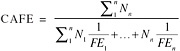 where Nn = number of vehicles in class n; FEn = fuel economy of class n vehicles; and n = number of separate classes of vehicles.