
3
Geodesy Requirements for Earth Science
Precise geodetic infrastructure enables ground- and space-based observations that are critical to a wide array of scientific disciplines, including seismology, geodynamics, climate science, hydrology, oceanography, meteorology, and space weather. Geodetic observations, for example, allow us to measure and monitor gradual changes in tectonic plate movement, sea level rise, glacial ice melting, and aquifer depletion. Similarly, the geodetic infrastructure provides the foundation for numerous applications with broad societal and commercial impact, from early warning systems for hazards to intelligent transportation systems (Figure 3.1). Over time, the precision and timeliness of these applications has improved, with operational applications now routinely working at accuracies only recently achievable, while the scientific applications are approaching the part-per-billion accuracy level and near-real-time operations. The scientific questions that are being asked about how the Earth system works and what can be predicted for the future continue to drive ever more stringent requirements for geodesy.
The demand for geodetic observations will continue to grow as we move from global to regional forecasts of climate change impacts, from manual to autonomous systems that require more precise positioning in real time, and from point positioning to geodetic imaging. Given the breadth of scientific and societal applications, this chapter is not intended to be comprehensive, but rather to highlight only a sampling of the benefits that high-precision geodetic infrastructure provides for Earth science and the nation.
SOLID EARTH DYNAMICS
Geodynamics
Plate Motion and Tectonics
Nothing on Earth’s surface is fixed, and enormous pieces of the crust are being ripped apart or forced into collisions with each other by the movement of the mantle below, causing earthquakes, volcanoes, and mountain building. Earth’s crust is currently considered to consist of approximately
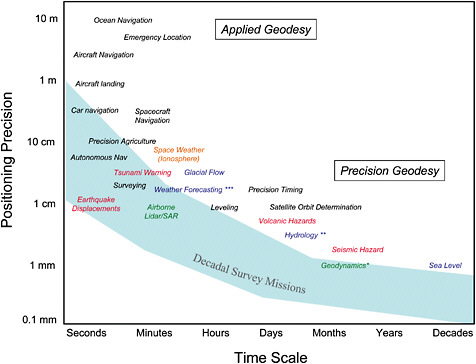
FIGURE 3.1 This schematic plots the precision of current geodetic applications as a function of the required time interval. The most demanding applications at the shortest time intervals include GNSS/GPS seismology and tsunami warning systems. At the longest time intervals, the most demanding applications include sea level change and geodynamics. Note that the positioning scale is in powers of 10 and that range of geodetic applications spans approximately nine orders of magnitude in the time scale. Consistency in connecting the longest to the shortest time scales requires an accurate and stable global terrestrial reference frame, which drives the most stringent requirements on the geodetic infrastructure.
* Plate motion, plate deformation, mountain building, mass transport, ice-sheet changes (using loading motion and gravity changes observed from space).
** Vertical surface motion from GNSS/GPS and InSAR for ground water management; water redistribution is monitored from space based on gravity measurements).
*** Water vapor and other meteorological information from GNSS/GPS ground stations and radio occultations in space.
52 “rigid” plates (14 major plates and approximately 38 minor plates) that slowly drift across the surface of the planet, changing speed and direction on million-year timescales (McKenzie and Parker, 1967). The edges of the plates undergo a variety of non-rigid and unsteady motions, which are classified according to the direction of relative plate motion across the boundary. Divergent boundaries form the mid-ocean ridges that encircle the planet like seams on a baseball. Here, plates spread apart and the void is filled from below by hot material. Convergent plate boundaries form the deep ocean trenches where the cooled plates subduct back into Earth’s mantle. The largest earthquakes occur when these subducting plates slip past each other after sticking together for a period of 300–1,000 years (stick-slip behavior). Transform boundaries (which cause strike-slip motion) mainly occur in the deep oceans, although they occasionally cut across the continental areas. A
prominent example of a transform boundary is the San Andreas Fault, which undergoes strike-slip motion on 100–1,000 year time scales, resulting in destructive earthquakes. Mountainous areas on the continents, such as the Himalayas and the Alps, are formed by convergent motion (collisions) between continental plates. However, where an oceanic plate collides with a continental plate, such as the North American Cascades, major earthquakes and volcanism can be expected.
Global-scale geodetic measurements of plate motions from Very Long Baseline Interferometry (VLBI) and Satellite Laser Ranging (SLR), based on less than a decade of data, show remarkable agreement (at the 3–5 millimeters per year level) with plate motions derived from the 1–3 million year average rates derived form the geological and geophysical data (Herring et al., 1986; Carter and Robertson, 1986). Some tectonic plate studies, however, drive a requirement for a higher level of accuracy. For example, the boundaries of the plates have narrow regions where shorter timescale plate-to-plate interactions are important. These include areas of high crustal strain (Figure 3.2), which result in destructive earthquakes and volcanoes. In addition, the plates do not behave exactly rigidly, and the measure of horizontal intraplate deformation could be associated with the thermal contraction of the cooling oceanic lithosphere. This plate shrinkage has recently been detected at the 3 millimeter per year level (Kumar and Gordon, 2009).
Post-Glacial Rebound
During the last Ice Age, vast ice sheets up to 4–5 kilometers thick lay over the Hudson Bay region in northern Canada and across much of Scandinavia. The amount of ice locked up in the ice sheets at the time was enough to cause global sea levels to lie 100–150 meters below their present levels (Peltier, 2004). The pressure from that ice load on Earth’s crust caused the underlying mantle to be depressed. When the ice melted, starting roughly 20,000 years ago and continuing until approximately 10,000 years ago for Canada and Scandinavia, Earth began to rebound. That rebound (also known as glacial isostatic adjustment) continues today because Earth is viscous, and it takes time for a viscous body to fully respond to the removal of a load. Observations of the rebound rate provide information about Earth’s viscosity profile, which plays a key role in determining the pattern and vigor of convection in Earth’s mantle that drives plate motion and causes earthquakes
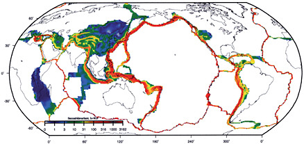
FIGURE 3.2 Geologic, geodetic, and earthquake data help determine the zones on Earth where the crustal motion diverges from rigid plate motion. Areas of high strain, in red, experience increased earthquakes and volcanoes. SOURCE: Kreemer et al., 2000.
and volcanic activity. The characteristics of the ancient ice sheets are also of interest because they provide insight into how the cryosphere has responded to dramatic changes in climate in the past.
It is only through geodetic observations that the present-day rebound can be observed as it actually happens. There are two types of relevant geodetic observations. One involves the measurement of surface uplift rates at points near the locations of the ancient ice sheets. Measurements of this type are now usually made with GNSS/GPS (see Lidberg et al., 2007; Sella et al., 2007), though VLBI observations have been used as well (Heki, 1996; James and Morgan, 1990; Mitrovica et al, 1993). The other type of geodetic observation is time-variable gravity. The ongoing rebound leads to changes in Earth’s mass distribution, which in turn cause Earth’s gravity field to evolve over time. The gravity field over northern Canada, for example, is steadily increasing in strength as mass in the underlying mantle flows in sideways from surrounding regions, pushing Earth’s surface upwards. Those gravity changes are best seen in satellite gravity data, such as from LAGEOS (Cox and Chao, 2002; Cheng and Tapley, 2004) and, especially, GRACE (see Box 3.1) (Paulson et al., 2007; Tamisiea et al., 2007). These space-based gravity measurement techniques use the geodetic infrastructure to determine an accurate reference against which to measure the small post-glacial rebound motions; the geodetic techniques also provide the data containing important geophysical signals.
Earth Orientation (Length of Day, Polar Motion, and Nutation)
The direction of Earth’s rotation axis and the rate of rotation about that axis vary with time (for general reviews, see Dehant, 2007; Gross, 2007; Lambeck, 1980). As described in Chapter 1, the change in the rate of rotation causes a small change in the length of day. The motion of the rotation axis itself is described by polar motion and nutation. Polar motion refers to motion of the axis relative to fixed points on Earth’s surface, while nutation refers to motion with respect to fixed objects in space. For the past several decades, the determination of Earth’s orientation has been based on observations from the global network of VLBI, GNSS/GPS, and SLR stations, and the results are critically dependent on reference frame accuracy. The orientation and rotation rate of the reference frame used when analyzing these geodetic measurements are directly related to the rotational parameters used for geophysical interpretation. Consequently, reference frame errors can map directly into errors in that interpretation.
Earth Tides
The tidal force from the sun and moon causes tides in the solid Earth, just as it does in the ocean. The periods are the same, and even the amplitudes are similar: tidal displacements in both the solid Earth and the open ocean are on the order of several tens of centimeters. Solid Earth tides are best observed using geodetic measurement techniques. Information on tidal deformation of Earth at global-scale wavelengths provides unique information on Earth’s structural parameters.
Natural Hazards
Volcanoes
There are 170 volcanoes in the United States, of which at least 65 are active or potentially active. The U.S. Geological Survey (USGS) Volcano Hazards Program routinely monitors volcanoes using a variety of methods designed to detect and measure changes caused by the underground movement of magma (molten rock). Rising magma typically will: trigger earthquakes and other seismic events; cause swelling or subsidence of a volcano’s summit or flanks; and lead to the release of
volcanic gases from the ground and vents. By monitoring these phenomena, scientists sometimes can anticipate an eruption days to weeks in advance or remotely detect explosive eruptions and lahars (a mixture of water and rock fragments that flow down the slopes of a volcano). Successfully monitoring and forecasting Mount Pinatubo’s cataclysmic eruption in 1991, for example, prevented property losses of more than $250 million (Newhall et al., 2005).
GNSS/GPS receivers and Interferometric Synthetic Aperture Radar (InSAR) are the main geodetic tools used for monitoring volcanic surface deformation, as well as earthquake deformation (discussed below). GNSS/GPS receivers can be set up at strategic locations around a site to stream measurements continuously. InSAR, on the other hand, can uniquely map and resolve surface deformation over a wide range of spatial scales that is not possible with GNSS/GPS (see Figure 3.3). The research community in the United States currently relies on InSAR data collected by several radar satellite missions, including those flown by the European (ERS-2, Envisat), Canadian (Radarsat-1) and Japanese (ALOS) space agencies (see Table 4.1). Combining the high-spatial-resolution InSAR map with high-temporal-resolution GNSS/GPS point measurements provides the full four-dimensional picture of volcanic deformation. An unexpected result of using InSAR and GNSS/GPS systematically to study volcanoes in Alaska and the western United States is the
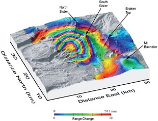
FIGURE 3.3 An InSAR-defined area of uplift near the Three Sisters cluster of volcanoes in central Oregon, where each concentric circle of red corresponds to approximately 28 millimeters in deformation. This deformation, which does not lie directly beneath any volcano, is in an area where the most recent eruption occurred 1,500 years ago. Uplift of the ground’s surface, which began in 1997, reached 15 centimeters at the center of the “bull’s eye” pattern in 2001. Subsequent GPS monitoring shows that uplift continues at a steady pace, suggesting that it is produced by upward movement of magma (intrusion). The InSAR pattern places the depth of intrusion at 6–7 kilometers. SOURCE: Wicks et al., 2002. Courtesy of the American Geophysical Union.
discovery that volcanoes once thought to be dormant are actually undergoing gradual deformation and may eventually erupt. Because volcanic deformation tends to be a slow process taking decades to centuries between eruptions, InSAR and GNSS/GPS measurements must be tied to decades of data from a stable terrestrial reference frame with better than 5 millimeter precision.
Earthquakes
The sudden release of energy along a major earthquake fault is one of the most destructive forces of nature. Predicting earthquakes depends on our ability to understand the earthquake cycle, which requires geodetic measurements of Earth’s crustal motion between seismic events. At depths greater than 20 kilometers, the North American and Pacific plates slide freely past one another. Shallow fault zones, however, are colder and more brittle and undergo stick-slip behavior, in which the shallow surfaces of the fault remain locked for periods sometimes lasting hundreds of years because of friction and surface imperfections. Eventually, the tectonic stress exceeds the fault strength, causing the plates to slip past each other (a coseismic event).
Recently, scientists discovered that slips can be either fast and destructive or slow and minimal. An example of short-term transient slow slip behavior at a subduction zone is the phenomenon of Episodic Tremor and Slip (ETS) (Rogers and Dragert, 2003; see Figure 3.4). ETS, as observed along the northern Cascadia Subduction Zone, has been defined empirically as repeated, transient ground motions at a plate margin. Prior to the discovery of ETS, geologists thought the Cascadia coastal margin was squeezed landward in a continuous, steady fashion. It is inferred that the deeper plate interface also undergoes a stick-slip behavior, but over a much shorter time-scale than the earthquake cycle. The relationship between ETS and regional earthquakes is not yet clear, but it is conceivable that an ETS episode could ultimately trigger a large earthquake.
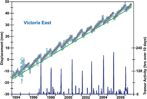
FIGURE 3.4 GNSS/GPS and seismic data as observed on the Cascadia Subduction Zone. The plot demonstrates an example of Episodic Tremor and Slip (Rogers and Dragert, 2003), a phenomenon of short-term transient slow slip behavior at a subduction zone. Each blue circle in the plot indicates the daily change of the east-west position of the Victoria GPS station relative to the interior of the North American Plate. The green line shows the long-term linear motion over the 14-year period. The red line shows that for roughly 15 months this deeper fault zone resisted slip but then slipped several centimeters over a period of weeks, resulting in a characteristic sloped saw-tooth time series for the longitude component of coastal GPS stations. SOURCE: Rogers and Dragert, 2003.
Fast ruptures generate elastic waves that propagate outward and destroy buildings. Slow ruptures, which could be detected only recently using GNSS/GPS receivers, can release the tectonic stress over periods of several days to weeks. Following an earthquake, the fault continues to slip, generating aftershocks. This postseismic deformation can last for tens of years.
Some scientists also hypothesize that there is a short period of concentrated deformation just prior to a major earthquake, although this period of preseismic deformation is poorly documented. Modern space-based geodetic measurements, such as GNSS/GPS and InSAR, have recorded all but the preseismic elements of the earthquake cycle. With the new tools geodesy offers, however, scientists are beginning to understand the earthquake process and may someday be able to provide useful earthquake forecasts.
Accurate and robust measurements of subtle secular and precursory deformation are the new frontiers in crustal deformation studies and are pivotal for natural hazards research. These measurements can be accomplished with GNSS/GPS, InSAR and Aircraft Laser Mapping (ALM). The Plate Boundary Observatory, part of the National Science Foundation’s EarthScope project, consists of 1,100 strategically distributed GPS receivers, as well as borehole seismometers, tiltmeters, and laser strainmeters installed along the western United States (see Figure 3.5). This geodetic observatory continuously monitors the strain field that results from the deformation of the active boundary zone
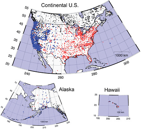
FIGURE 3.5 Map showing the continuously operating GPS stations in the United States. Blue dots are Plate Boundary Observatory (PBO) sites installed by the NSF. Red dots are Continuously Operating Reference Stations (CORS), which are installed and operated by a variety of federal, state, and local agencies and some private companies and whose data is available through the National Geodetic Survey. Black dots are other sites that do not fall into either the PBO or CORS groups. Some of the PBO sites are also CORS sites. SOURCE: Courtesy of Thomas Herring, Massachusetts Institute of Technology, using Generic Mapping Tool (GMT developed by Paul Wessel and Walter Smith). Graphic generated on May 28, 2010, using NOAA/NGS CORS data acquired from CORS website: http://www.ngs.noaa.gov/CORS/sort_sites.shtmll.
over multiple time scales. InSAR is a highly complementary and synergetic technique to the Plate Boundary Observatory’s GPS network, because it can generate continuous high-resolution maps of surface strain over large areas in any weather condition day or night, typically on monthly timescales. Figure 3.6, based on InSAR data, illustrates the ground deformation resulting from the 7.9-magnitude Wechuan earthquake in China. Precise orbits and ionospheric delay corrections are needed to construct a seamless deformation map from multiple swaths. ALM offers a third geodetic method for estimating seismic hazards. The B4 project, for example, has mapped the entire San Andreas fault system at 1-meter spatial resolution and 0.1 meter vertical accuracy. Studies of the morphology of the fault zone, such as those combining offset stream channels with geochronology, provide critical information on the recent slip histories of specific faults. This information can be compared with the strain accumulation rate measurements from geodesy to estimate when the next major rupture is most likely to occur. In addition, mapping that is done before the next major rupture (hence, “B4”) will
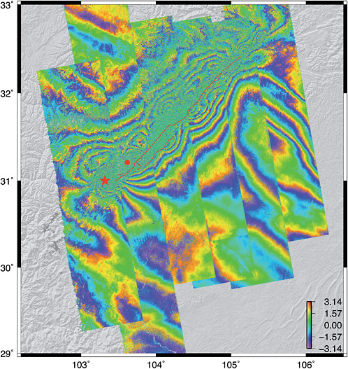
FIGURE 3.6 Ground deformation from ALOS L-band interferometry (each concentric color “fringe” corresponds to approximately 10 centimeters of displacement) due to the 7.9-magnitude Wenchuan earthquake, which occurred on May 12, 2008, along the western edge of the Sichuan Basin in China. Shaking from the 270-kilometer-long rupture destroyed thousands of structures, killing nearly 70,000 people and leaving more than 4.8 million homeless. ALOS-derived ground deformation maps were available within a few days after the rupture in order to assess the extent of the damage zone, as well as to provide an estimate of regions of increased seismic risk. SOURCE: David Sandwell, University of California–San Diego.
provide the reference surface for assessing the very-small-scale deformation associated with a major rupture. The geodetic infrastructure for earthquake hazard monitoring with GNSS/GPS, InSAR and ALM would require better than 5-millimeter accuracy over 10 years.
Landslides
Landslides include a wide range of ground movements, such as rock falls, deep failure of slopes, and shallow debris flows (USGS, 2010). Although gravity acting on an over-steepened slope is the primary reason for a landslide, there are other contributing factors such as soil saturation by rainfall or snowmelt, earthquakes, volcanic eruptions, and stress induced by man-made structures. Understanding and mitigating landslide risk involves identifying areas of susceptibility (see Radbruch-Hall et al., 1982), determining which potential landslides are active, and deploying ground-based investigations in area of high risk and/or active slide areas.
A promising method for identifying active landslide areas greater than about 200 meters is to use InSAR. Newer Japanese InSAR satellites operating at a longer wavelength (L-band) may make it possible to perform a global inventory of active landslides, even including those on vegetated surfaces. When the location of an active slide has been determined, ground-based methods, such as Light Detection and Ranging (LiDAR) mounted on tripods or aircraft, can be deployed to obtain “bare Earth” surveys (see Figure 3.7). The three-dimensional coordinates of the laser points can be used to determine the volume of the material involved in the landslide, as well as surface roughness and slopes of the slide and surrounding terrain.
Floods
Many natural processes, including hurricanes, weather systems, and snowmelt, can cause floods. Floods can also be caused by failure of levees and dams and inadequate drainage in urban areas.
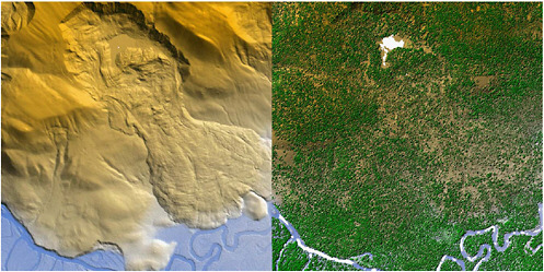
FIGURE 3.7 These false-color geodetic images of a landslide near Flathead Lake, Montana, were made from airborne LiDAR data collected by the NSF National Center for Airborne Laser Mapping (NCALM). Laser shots passed through openings in the forest and reached the ground, allowing a filter to be used to remove the returns from the trees and reveal the landslide, which is not normally visible to the eye or a camera. The white scale bars are 500 meters in length. SOURCE: Ramesh Shrestha, National Center for Airborne Laser Mapping (NCALM), University of Houston; see also Carter et al., 2007.
On average, floods kill more than 100 people in the United States each year and cause billions of dollars in property damage (Figure 3.8). Land surface elevation defines the direction, velocity, and depth of flood flows, while subsidence measurements indicate how these values will change in the future. Elevations of individual streams and rivers traditionally have been mapped by land surveying. However, because Federal Emergency Management Agency (FEMA) floodplain mapping must cover nearly one million miles of the nation’s streams and shorelines, land surface elevation data are mostly derived from mapped sources, not from land surveying (NRC, 2007b). Land surface elevation information is combined with data from flood hydrology and hydraulic simulation models to define the base flood elevation, which indicates the extent of inundation. The creation of floodplain maps is an important part of the National Flood Insurance Program, as these maps determine flood insurance requirements. FEMA is undertaking an ambitious five-year program to update and digitize the nation’s floodplain maps.
Flat terrain in coastal zones and river flood plains are particularly flood-prone. According to the National Research Council (NRC) report Elevation Data for Floodplain Mapping (2007b), “…elevation data of at least 1-foot equivalent contour accuracy should be acquired in these very flat areas, rather than the 2-foot equivalent contour accuracy data that the FEMA floodplain mapping standards presently require for flat areas.” Achieving this 1-foot accuracy actually requires two geodetic measurements—the terrain elevation and the geoid height (see Chapter 1). The NRC
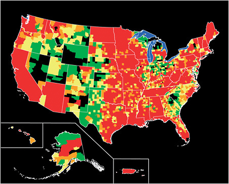
FIGURE 3.8 Presidential disaster declarations related to flooding in the United States, shown by county: Green areas represent one declaration; yellow areas represent two declarations; orange areas represent three declarations; and red areas represent four or more declarations between June 1, 1965, and June 1, 2003. Map is not to scale. SOURCES: FEMA; Michael Baker Jr., Inc.; the National Atlas; and the USGS (from http://www.usgs.gov/hazards/floods/).
committee examined three technologies for supplying elevation information: photogrammetry, LiDAR, and InSAR. LiDAR is capable of producing a bare-Earth elevation model with two-foot equivalent contour accuracy in most terrain and land cover types; a four-foot equivalent contour accuracy is more cost-effective in mountainous terrain, and a one-foot equivalent contour accuracy can be achieved in very flat coastal or inland floodplains. A seamless nationwide elevation database created at these accuracies would meet FEMA’s published requirements for floodplain mapping for the nation. The second geodetic measurement needed to achieve the one-foot contour accuracy requirement is the geoid height. Water flows downhill with respect to the geoid, which coincides with mean sea level at the coastline, or zero elevation. The combined accuracy of the terrain elevation and geoid height is approximately 30 centimeters, so the geoid accuracy alone must be better than that. The latest high-resolution global geoid height model EGM2008 (see Chapter 4) is estimated to be accurate to 10 centimeters or better over most of the United States (Pavlis et al., 2008a), which meets the geoid height accuracy requirement.
Tsunamis
Some of the most catastrophic natural disasters result from tsunamis. Tsunamis are generated by rapid displacement of the ocean floor (Song et al., 2008). The largest tsunamis are generated by earthquakes, specifically megathrust earthquakes occurring at ocean trenches known as subduction zones, where tectonic plates converge. Such was the case for the Indian Ocean tsunami, which was generated by an estimated 9.1- to 9.3-magnitude Sumatra earthquake (Stein and Okal, 2005), killing more than 150,000 people and leaving millions more homeless in 11 countries (National Geographic News, 2005). Subduction zones that present the largest tsunami hazard risk in the United States are those of the Pacific Rim, Alaska, and Cascadia, which is off the coast of Oregon and Washington.
Understanding the mechanism for tsunami generation is the key to assessing where future tsunamis are likely to occur and to developing early warning systems. A tsunami warning system will require the installation of continuously operating geodetic GNSS/GPS networks, which stream data in real time, as well as data analysis centers capable of processing the data in near real time. As illustrated in Figure 3.9, by measuring the rapid horizontal displacement of a GNSS/GPS receiver near the coast of a subduction zone, scientists can infer how much slip has taken place during the earthquake at the interface of the tectonic plates. From models of how earthquakes deform Earth’s surface (Wang, 2003), it is possible to predict how much energy is imparted to the ocean, and thus
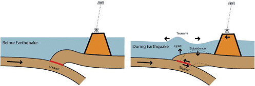
FIGURE 3.9 The largest tsunamis are generated by earthquakes occurring at ocean trenches, known as subduction zones, where tectonic plates converge. If the rapid horizontal displacement of a GNSS/GPS receiver near the coast of a subduction zone was measured and immediately available, it would be possible to infer how much slip had taken place and predict the likely size of the resulting tsunami. SOURCE: Blewitt et al., 2009.
predict the initial conditions of tsunami generation (Song, 2007). Ocean dynamic models can then be used to predict the ensuing tsunami (Titov et al., 2005). The key to this method is to be able to accurately measure the rapid horizontal displacement of GNSS/GPS receivers at the time of the earthquake.
Progress is being made to develop this capability. In the United States, the operational Global Differential GPS (GDGPS) System, developed by NASA’s Jet Propulsion Laboratory (JPL) (Muellerschoen et al., 2001), is currently delivering real-time GPS corrections and is being developed into a system to enable real-time positioning with few-centimeter accuracy. Similarly, the International GNSS Service’s Real-Time Pilot Project has the potential to demonstrate precise real-time positioning. In Canada, a pilot project is underway to measure, in real-time, the displacement of coastal GPS stations relative to stations further inland (Dragert et al., 2005). In Japan, the Earthquake Research Institute has developed tsunami warning buoys that are tracked by GNSS/GPS (Kato et al., 2005). In addition, Japan’s Geographical Survey Institute already has GEONET, a very dense GNSS/GPS network with a real-time capability (Yamagiwa et al., 2006). In Europe, GeoForschungsZentrum has developed a concept known as “GPS Shield” (Sobolev et al., 2007), which also includes coastal GNSS/GPS stations as well as GNSS/GPS-tracked buoys to observe tsunamis directly. Accurate real-time GNSS/GPS geodesy requires near-real-time determination of GNSS/GPS satellite and clock parameters, a capability that is already under development by NASA at JPL. There is a need for interagency cooperation between NASA and NOAA to facilitate the transfer of this near-real-time information on tsunami-generating earthquake sources (NRC, 2011). A similar cooperation between NASA and USGS could facilitate rapid estimation of shaking and damage on land caused by large earthquakes. Figure 3.10 demonstrates that, had a real time capability for GNSS/GPS
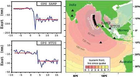
FIGURE 3.10 Permanent displacements observed using GPS during the estimated 9.1- to 9.3-magnitude Sumatra earthquake in 2004 demonstrated that, within minutes, permanent displacements can be resolved with approximately 10-millimeter accuracy. Sites SAMP and NTUS in the near-field (within approximately one rupture length) provide statistically significant offsets from which earthquake magnitude can be determined (left) to be in the range capable of generating an ocean-wide tsunami (right). The yellow star is the earthquake epicenter. Units of the x-axis on the GPS seismograms (left) are minutes with respect to source time of the earthquake. SOURCE: Adapted from Blewitt et al., 2009.
measurements been available in 2004, the displacement of stations in Sumatra could have been measured with centimeter-level accuracy within minutes and thus could have indicated the true magnitude and tsunami potential of the Sumatra earthquake (Blewitt et al., 2006), thereby allowing for some warning.
OCEAN DYNAMICS
Geodesy, specifically satellite altimetry, in which a radar pulse is used to measure sea surface height, is critical to the study of ocean processes and their impacts on Earth’s climate. Sea surface height measurements from the Topex/Poseidon and Jason-1 and Jason-2 missions are currently assimilated into global ocean circulation models to provide realistic information on the three-dimensional ocean circulation and state, as well as how those factors change over time (see Carton et al., 2008; Wunsch et al., 2007). Data assimilation (in particular the assimilation of altimetry data) into Ocean General Circulation Models is currently performed for operational oceanography, allowing ocean forecasting analogous to meteorological forecasting. In 1997–1998, the Topex/Poseidon satellite monitored an El Niño-Southern Oscillation (ENSO) event, offering the first space-based observation of such an event from its initialisation to its decay (see Fu and Le Traon, 2006). These observations helped clarify the role of equatorial waves in the movement of the warm pool, leading to significant revision of existing ENSO theories.
Satellite altimetry, which supplies continuous worldwide observations, also has considerably increased our knowledge of large-scale ocean circulation through mapping of the ocean surface topography (Fu and Chelton, 2001). Historically, geoid errors were the most limiting factor for precisely determining the ocean surface topography, and hence the large-scale surface circulation from which the deep circulation can be derived. The situation has considerably improved with precise geoid estimates based on the GRACE space gravimetry mission; further improvement is expected from the Gravity Field and Steady-State Ocean Circulation Explorer, launched by the European Space Agency in 2010. Among the most important discoveries from satellite altimetry is the strong mesoscale ocean variability observed almost everywhere in ocean basins, indicating that eddy energy generally exceeds the energy of the mean flow by an order of magnitude or more. Observations on this variability have provided new insights into eddy dynamics and the role of eddies in ocean circulation, heat, and salt transport (Fu and Ferrari, 2008).
Sea Level Change
One of the most important problems being monitored by satellite altimetry and tide gauges is the change in global and regional sea levels. Mean sea level rise has been observed by tide gauges for well over a century, but the global mean rate of sea level rise appears to be increasing over the more recent time periods. As shown in Figure 3.11, the observed global mean sea level rise was on the order of 1 millimeter per year from the late 19th century to the early 20th century, but then the rate appears to have doubled to 2 millimeters per year. During the past decade, this rate appears to have increased to approximately 3 millimeters per year. This significantly higher rate has been confirmed (see Figure. 3.12) by the series of ocean altimeter missions starting with TOPEX/Poseidon and continuing with Jason-1 and Jason-2 (Ablain et al., 2009; Beckley et al., 2007; Leuliette et al., 2004). In addition, regional sea level rise can be even more severe due to changes in large-scale ocean circulation patterns (see Yin et al., 2009).
A number of error sources have to be considered when interpreting the apparent global mean sea level rise, either from tide gauges or altimeter missions. For the tide gauges, the limitations are primarily the geographical distribution of the measurements (necessarily limited to coastal regions), and uncertainty in the vertical motions of the tide gauges themselves. With space-based altimeters, the
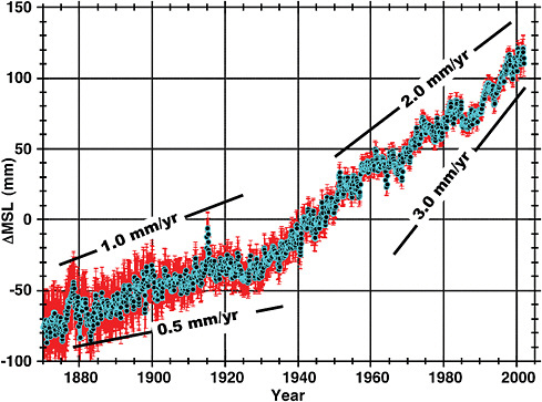
FIGURE 3.11 Sea level rise estimated from global tide gauge measurements. The average rate over the 1970–2010 period covered by the measurements has been approximately 1.7 mm/yr. However, the rate has clearly been accelerating over that period, as evidenced in the data by marked increases in slope. SOURCE: J.B. Minster, adapted from Church and White, 2006.
global ocean can be sampled much more uniformly, but a number of errors sources arise. Improvements to the global geodetic infrastructure will reduce these errors, improving our predictive capability.
Table 3.1 provides an estimate of the systematic errors in measuring the global mean sea level rise from altimeter data (adapted from Nerem, 2009). See also Ablain et al. (2009), where the details are slightly different but the net error is similar (approximately 0.4–0.6 millimeters per year). The altimeter drift error includes several components, predominantly the calibration of the microwave radiometers used for the wet troposphere correction. The reference frame errors can bias the results through drifts in the satellite orbits due to reference frame origin errors (see Beckley et al., 2007). For this particular error, there is considerable cancellation in the global value due to nearly equal and opposite contributions from the northern and southern hemispheres (they would cancel exactly if there was the same amount of ocean area in each hemisphere). Errors in regional sea level changes can be considerably larger than the global mean, exceeding one millimeter per year at the higher latitudes (Beckley et al., 2007). Since the slope of the shoreline amplifies the impact of the vertical change in apparent sea level, it is the regional sea level change that is critical for hazard assessment and mitigation. Another significant source of error is the altimeter calibration based on tide gauges that may have a common vertical rate error due to a reference frame scale error (Tapley and Ries, 2005). Unfortunately, for many tide gauges, there is no measurement of the vertical rate (whether uplifting, subsiding, or steady), and this also contributes to the uncertainty in the tide gauge calibration of the altimeter biases and drifts (Mitchum, 2000).
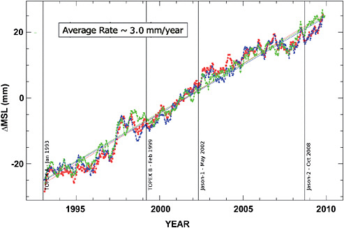
FIGURE 3.12 Three different determinations of sea level changes from the ocean altimeter missions TOPEX/Poseidon, Jason-1, and Jason-2 (M. Ablain, personal communication). The slope is the global mean sea level after correction for glacial isostatic adjustment. The vertical lines indicate important mission transitions; each represents a relative bias that must be determined through tide gauge calibration or through overlapping data analysis. Data from the University of Colorado (S. Nerem), blue curve; from the Goddard Space Flight Center/NASA (B. Beckley), red curve; and the Collecte Localisation Satellites-Laboratoire d’Etudes en Géophysique et Océanographie Spatiales (M. Ablain), green curve. SOURCE: Courtesy of M. Ablain, CLS, Collecte Localisation Satellites, Toulouse, France.
The uncertainty in estimates of global mean sea level can be compared to the two primary contributors to sea-level rise, thermal expansion, and ice melt. Over the altimetry time span (1993–2009), approximately one-third of the rise is attributed to the thermal expansion and two-thirds to melting of mountain glaciers and the polar ice sheets (Cazenave and Llovel, 2010; Leuliette and Miller, 2009; Nerem et al., 2006). The uncertainty from the reference frame and tide gauge vertical motion errors, up to 0.4 millimeters per year, is a considerable fraction of this mass loss estimate. The rate at which fresh water from ice melt is entering the oceans is a critical component of understanding what is causing the apparent acceleration of global mean sea level rise. There also is evidence that Greenland and Antarctica are losing ice mass at an accelerating rate (Chen et al., 2009; Jiang et al., 2010; Shum et al., 2008; Velicogna, 2009) and that the contribution to sea level rise from that loss will consequently increase further.
It is extremely important to identify and understand the sources of the current rise in global mean sea level, so that climate models can accurately reflect actual climate change processes. Consequently, precise geodetic measurements of the change in ocean volume (from radar altimetry), ocean temperature and salinity (from in situ instruments such as Argo), ice sheet mass balance (elevation change from radar and laser altimetry, coastal glacier flow from InSAR, and mass change from GRACE space gravimetry), and ocean mass (from space gravimetry) are all important pieces of the observational framework to test the validity of ice dynamic and ocean temperature change
TABLE 3.1 Estimate of Dominant Systematic Errors Sources in Measuring Global Mean Sea Level Rise from Space-based Altimeters
|
Altimeter Global Mean Sea Level Measurement Error Budget |
|
|
Glacial isostatic adjustment (affects volume of ocean basins) |
0.1 mm/y |
|
Altimeter drift error (predominantly radiometer drift) |
0.4 mm/y |
|
Altimeter bias errors (the ability to link overlapping missions) |
0.4 mm/y |
|
Reference frame origin error (affects the satellite orbits) |
0.2 mm/y |
|
Systematic vertical motion error (affects the altimeter calibration) |
0.4 mm/y |
|
Total error (root-sum-squared) |
0.6 mm/y |
models (see recommendations of the 2009 OCEANOBS workshop; Cazenave et al., 2010). All of the space-based techniques rely on an accurate reference frame, so maintaining and improving the accuracy of the terrestrial reference frame is of paramount importance for the study and for understanding global sea level rise. Ongoing research on altimeter drift and bias errors can be expected to reduce those uncertainties. The reference frame errors, however, are outside of the control of the altimeter data analysts and must be addressed by the geodetic community through improvements in the geodetic networks and the analysis of the data provided by those networks.
ICE DYNAMICS
One of the most dramatic effects of global change is the melting of ice from continental glaciers and polar ice sheets. Mountain glaciers around the globe have been in fast retreat for the past few decades, and observations indicate that the Greenland and Antarctic ice sheets are beginning to lose mass at alarming rates (Lemke et al., 2007). The acceleration of ice loss in Greenland and Antarctica was not widely anticipated before it was observed, and explanations to account for this acceleration are still incomplete. Only through careful monitoring of the ice sheets—using techniques that rely heavily on geodetic infrastructure—was the acceleration noticed and quantified. The continued application of current and future geodetic techniques is required for the scientific community to be able to monitor the ice sheet mass balance at the accuracy needed to understand what is happening today and to develop models for predicting future ice sheet mass changes. Of particular importance is the systematic application of geodetic imaging techniques that use radar and LiDAR to produce images of the Earth’s surface wherein the location each pixel is known with geodetic precision, so that the difference between two pictures of the same area can be interpreted geologically and physically.
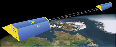
Information about the mass balance of the ice sheets is based on four types of remote sensing and ground techniques: (1) elevation change of the ice sheet, as measured by laser altimetry (for example, IceSAT), satellite radar altimetry (for example, ERS, EnviSat), and ground-based GNSS/GPS receivers; (2) measurements of horizontal velocities near the grounding line (where the ice starts to float free of its bed) of outlet glaciers using either on-ice GNSS/GPS receivers or satellite-based InSAR (for example, ERS, Radarsat, Envisat, ALOS satellites); (3) changes in the gravity field above the ice sheet, as measured by space-based gravimetry; and (4) geodetic measurements (for example, GNSS/GPS, gravity) of vertical motions in deglaciated areas. Monitoring changes in ice sheet elevation provides a direct estimate of changes in ice sheet volume, from which mass change is deduced based on the density through the snow/ice column. However, an accurate orbit is needed to achieve these calculations, which in turn depends on the accuracy of the reference frame. The GRACE mission (see Box 3.1) uses satellite-to-satellite tracking, as well as measurements from onboard GPS receivers and accelerometers, to determine global, monthly gravity solutions. These solutions can be used to map monthly changes in the distribu-
tion of mass at Earth’s surface, and to determine the mass variability of Greenland, Antarctica, and major mountain glacier systems (for example, Alaskan coastal glaciers). The mass changes in Greenland from 2003 to 2008 are illustrated in Figure 3.13. The availability of data from a worldwide network of GNSS/GPS receivers is a critical component in the ability for GRACE to monitor these important mass changes.
To interpret space gravimetry and altimetry data over the ice sheets, it is necessary to correct for post-glacial rebound, also called glacial isostatic adjustment. This is corrected using models or by making direct GNSS/GPS measurements of the crustal motion on the ice-free land adjacent to the ice sheet. Each of these techniques involves geodetic instrumentation and relies critically on the geodetic infrastructure. Post-glacial rebound measurements by GNSS/GPS on ice-free land also require accurate reference frame determinations.
HYDROLOGIC CYCLE AND WATER RESOURCES
An overarching goal of observational hydrology is to better understand how water is transported and stored on and beneath the land surface. Traditional hydrological observations do not typically employ geodetic techniques, but with the advent of high-precision geodetic measurement systems, most of which depend heavily on the geodetic infrastructure, new and innovative methods for probing hydrological processes are providing valuable new information and hold great promise for the future.
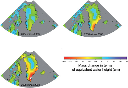
FIGURE 3.13 Mass changes in the Greenland ice sheets observed by GRACE. Observing the differences in the gravity fields determined in successive years reveals an ongoing loss of ice mass in Greenland, especially along the southeastern coast. There is evidence that the northwestern coast is now also losing mass. SOURCE: The University of Texas Center for Space Research.
Surface and Groundwater Storage
A change in water storage, on the surface or underground, involves a change in mass, which causes a corresponding change in the gravity field. The total change in water mass, therefore, can be estimated by measuring the change in gravity. These measurements can be made either from satellites or from surface gravity meters. The GRACE satellite mission, for example, is providing estimates of seasonal, yearly , and long-term changes in water storage at spatial scales of a few hundred kilometers and greater, to accuracies approaching one-centimeter water thickness, everywhere over Earth’s surface. The results can be used to monitor the amount of water stored in underground aquifers (see Figure 3.14) and to assess and improve hydrological models. For example, the United States Drought Monitor and the North American Drought Monitor rely heavily on precipitation data and subjective reports. As GRACE data are combined with other observations and hydrology models, they will help improve these drought monitoring products and prediction tools. The GRACE results also will help to determine the role of continental water variability in global mean sea level change and to better understand the transfer of water between the land and the atmosphere (precipitation and evaporation) at regional scales (see Frappart et al., 2006; Rodell et al., 2007; Swenson and Milly, 2006; Swenson et al., 2006; Zaitchik et al., 2008). For shorter-scale information, surface gravimeters, which sit on Earth’s surface and measure gravity changes directly at the instrument, are sensitive to changes in water storage averaged vertically through the ground directly beneath the meter (see Jacob et al., 2008; Van Camp et al., 2006).
Subsidence and Surface Displacement
In many cases, the vertical motion of the ground is caused by water storage changes. Various mechanisms can contribute to these changes. For example, when water storage decreases, the corresponding weight on Earth’s surface decreases, and so the surface can rise. Alternatively, if water is drained from pore spaces underground, the pore spaces can contract, causing the overlying surface to drop (subside). A surface gravimeter will record a signal not only if there is an underlying change in mass, but also if the surface on which the meter sits goes up or down. In the latter case, gravity will change because the meter moves further or closer to Earth’s center. This effect can confuse the interpretation of the results in terms of mass change, and so the vertical displacement of the surface is usually monitored independently, typically using GNSS/GPS receivers (van Dam et al., 2001). For example, local government agencies in Houston, in collaboration with the National Geodetic Survey, have established a network of permanent GPS receivers to monitor groundwater-related subsidence around the city (Zilkoski et al., 2001). Observations such as these not only provide indirect measurements of the aquifer drawdown but also help city planners understand and manage the possible effects of surface subsidence. GNSS/GPS results have even been used to estimate global-scale water storage by combining uplift measurements from globally distributed GNSS/GPS receivers (see Blewitt et al., 2001; Wu et al., 2003).
Groundwater-related surface motions also can be monitored using satellite or airborne InSAR measurements. Permanent GNSS/GPS stations provide continuous time-dependent displacements, but only at discrete points. In contrast, InSAR provides displacements over an entire region of tens of kilometers or more, though only at times when the satellite passes overhead (see Amelung et al., 1999; Buckley et al., 2003; Bawden et al., 2001). An example InSAR image of surface subsidence of New Orleans is shown in Figure 3.15. The subsidence is attributed to drainage projects that cause soil desiccation and oxidation, leading to compaction (Dixon et al., 2006). Data such as these provide information on the nature of the subsidence and on the possible hazards associated with that subsidence.
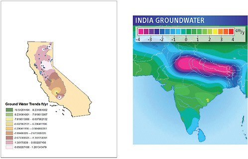
FIGURE 3.14 Major groundwater loss in the Sacramentro–San Joaquin River Basins in California (left) (Strassberg et al., 2009) and northern India (right) (Tiwari et al., 2009) revealed by the GRACE gravity mission and supplementary data. SOURCES: California groundwater iamge, NASA, http://www.nasa.gov/topics/earth/features/graceImg20091214.html (Left). India groundwater image, ScienceNOW, adapted from Tiwari et al., 2009 (Right).
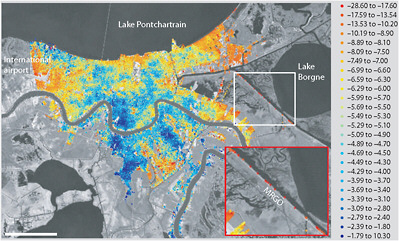
FIGURE 3.15 Map showing surface uplift rates (scale on right; units are millimeters per year) of New Orleans for 2002–2005, obtained from an InSAR analysis. Negative values for the uplift rates indicate subsidence. Most of New Orleans is subsiding relative to the global mean sea level, at an average rate of about 8 millimeters per year. Inset shows high subsidence rates between 2002 and 2005 on the MRGO levee, which later failed catastrophically during Hurricane Katrina. SOURCE: Dixon et al., 2006.
River and Lake Levels
In spite of the limitations of nadir-viewing radar altimetry (as opposed to side-looking radar imaging), monitoring surface water levels of rivers and lakes from space has a number of hydrological applications. These include studying the spatial and temporal effects of climate variability on surface waters, in particular over international river basins; improvement of models used in forecasts of hydrological variability; and water resource management (see Alsdorf and Lettenmaier, 2003; Cretaux and Birkett, 2006; Calmant and Seyler, 2006). Over floodplains, the combination of altimetry-based water levels with radar or visible satellite imagery allows scientists to monitor changes in surface water volume, particularly during floods (see Frappart et al., 2006). Laser altimetry (for example, the Ice, Cloud, and Land Elevation Satellite, or ICESat, mission) is also being used. More than 15 years of radar altimetry measurements are now available for several thousand continental lakes, as well as for “virtual stations” on rivers (the intersection of the satellite ground track and the river) and floodplains. Typical height precision over lakes, where data from several altimetry missions can be combined, is a few centimeters. Over rivers, altimetry-based height precision is less accurate (in the range of 10–40 centimeters) for two reasons: (1) only those data that come from repeat passes over the same satellite track can be combined in a single analysis, so there is limited data available except along very large rivers, and (2) because of the large radar footprint, reflections from river banks perturb radar echoes (waveforms); moreover, unlike for oceans, there is no simple interpretation of river waveforms.
A new concept of wide-swath radar interferometry has been recently proposed (Alsdorf et al., 2007) to monitor surface waters with unprecedented resolution (of approximately 100 square meters) and provide global coverage of worldwide rivers, lakes, and floodplains every few days. This mission, called SWOT (Surface Water Ocean Topography), was recommended by the NRC “Decadal Survey” and is listed among NASA’s future priority missions. SWOT will open a new
era in land hydrology, offering important new perspectives for studies on the terrestrial water cycle, flood prediction, and water resources.
WEATHER
Satellite imagery shown on television can give the impression that weather forecasts are based on these images, but forecasts actually come from physics-based models of the troposphere, the lowest 14 kilometers of the atmosphere. These models must continuously ingest measurements of the atmospheric state (pressure, temperature, humidity, and winds) at different altitudes around the planet to stay aligned with actual atmospheric conditions. The ability to predict both the severity and the temporal and spatial extent of weather changes, especially precipitation, is critical for public safety and agriculture, and governments around the world collaborate to collect the data used in forecasts. For decades, the input data for these models were provided by radiosondes, better known as weather balloons. Unfortunately, the spatial distribution of radiosonde sites is limited both by lack of coverage over oceans and by a significantly reduced number of sites in the southern hemisphere. Increasing the number of radiosonde launches per day is constrained by the cost of the instrumentation, which cannot be reused. Geodesists focused on precise positioning use corrections to remove atmospheric effects, which are considered to be a source of noise in their measurements. Conversely, these same corrections may be used by meteorologists to better understand the atmosphere. Thus, improvements in the geodetic infrastructure benefit both fields of science.
Ground-based Measurements
Atmospheric refraction effects have long been recognized as an important error source in geodesy. Instead of relying upon uncertain models, space geodetic techniques such as GNSS/GPS estimate tropospheric variations along with the positioning parameters of interest. Eventually, it became possible to reverse the problem; assuming that the station position is well-determined, scientists could use the “nuisance” signal in the GNSS/GPS estimates to recover the time-varying behavior of the atmosphere (Ware et al., 2000). Unlike radiosondes, which measure the atmosphere conditions at multiple altitudes, ground-based GNSS/GPS measures only the “integrated” effect of the atmosphere, that is, how much the atmosphere delays the measurement in total. About 80 percent of the delay (known as the “dry troposphere”) can be predicted if surface pressure is measured. Once the dry troposphere delay is removed, one can recover the delay due to water vapor, which can be scaled to what is called precipitable water vapor (PWV). Measurements of PWV estimate moisture and latent heat transport models, which are critical for weather forecasts. To be useful for weather forecasting, however, the data must be available at close to real time.
Since PWV varies both in space and time, globally distributed and frequently collected data are needed. For the current constellation of approximately 30 satellites, a single GNSS/GPS receiver will typically receive signals from 6 to 12 satellites. These data are primarily used to estimate PWV in the column of air above the GNSS/GPS receiver. But, in principle, having measurements from more than one direction means that GNSS/GPS has azimuthal, as well as vertical, sensitivity. The more satellites that are transmitting signals from a given direction, the greater the sensitivity will be. This also means that the combination of signals from multiple systems, such as Galileo, GLONASS, and COMPASS, will yield even more sensitive atmospheric monitoring capabilities than are achievable from the United States’ GPS alone. In addition, because GNSS/GPS receivers operate continuously, GNSS/GPS atmospheric sensing has extraordinary temporal sensitivity, which is particularly important for monitoring and predicting the behavior of strong weather events.
Because the atmospheric delay is intrinsically related to how well position can be determined, GNSS/GPS tropospheric studies require the same infrastructure: accurate orbit determination, along
with a stable reference frame. Atmospheric applications require a co-located barometer to allow removal of the pressure, or “dry troposphere,” effect. Well-designed sites with low multipath errors are also valuable as they will produce more accurate estimates of PWV. For weather prediction, however, there is the additional requirement that accurate orbits must be available in real time, whereas for climate studies, orbits can be made available in days to weeks. In order to achieve real-time accuracy, a reliable, globally distributed network of at least 50 real-time GNSS/GPS sites must be maintained. Rapid analysis of the data produced by this tracking network also must be supported (see Chapter 4). In order to improve the value of the large number of existing GPS receivers in the United States for meteorology, real-time telemetry capabilities would need to be expanded.
Space-based Measurements
While GNSS/GPS receivers have much greater temporal sensitivity than radiosondes launched twice per day, GNSS/GPS receivers have similar spatial limitations, in that they are (currently) limited to land and are present mostly in the northern hemisphere. For this reason, the atmospheric science community has actively sought measurements with better spatial density in the southern hemisphere and over the oceans. In the early 1990s, it was proposed that limb-sounding, a method that had been used to sense planetary atmospheres, could provide spatially dense measurements of Earth’s atmosphere. In a limb-sounding, or radio occultation, experiment, a radio signal is tracked from space rather than from Earth (Figure 3.16). This means that the horizon restriction is eliminated, and the signal can be refracted through the atmosphere for very long distances. The more GNSS/GPS and low-Earth orbit satellites are available, the more occultations that can be retrieved per day.
After the success of a proof-of-concept satellite mission in the late 1990s (Kursinski et al., 1996), the six-satellite Constellation Observing System for Meteorology Ionosphere and Climate
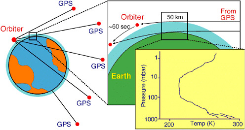
FIGURE 3.16 Schematic of a GNSS/GPS radio occultation, or limb-sounding, measurement. Signals transmitted by a GNSS/GPS satellite are refracted by the atmosphere and received by the orbiter, generating a vertical profile of pressure and temperature through the atmosphere until the signal is eventually blocked (occulted) by Earth. SOURCE: Yunck, 2002.
(COSMIC) was launched in 2006. Now operational, COSMIC provides global three-dimensional coverage of atmospheric temperature and water vapor from Earth’s surface to 40 kilometers (Anthes et al., 2008). In one day, COSMIC produces more than 1,000 well-distributed “soundings” in the southern hemisphere, compared to just over 100 southern hemisphere radiosondes above the continents. Furthermore, COSMIC is an all-weather system, and thus provides crucial data from the polar regions, observations for which are currently limited by weather restrictions. These new GNSS/GPS occultation data reduce uncertainties in both global and regional weather analysis and are routinely assimilated into both U.S. and European weather forecast models. In order to operate properly, however, they have requirements similar to those of ground-based GNSS/GPS networks, including accurate orbits and reference frame (which require a global GNSS/GPS tracking network providing near-real-time data). In addition, the velocity of the GNSS/GPS satellite relative to the low-Earth orbit satellite must be known to 0.1 millimeters per second, placing stringent demands on near-real-time orbit determination precision.
SPACE WEATHER
Above altitudes of 70–400 kilometers, the atmosphere is so thin that free electrons can exist. This ionized portion of the atmosphere contains a plasma—the ionosphere—in which the magnitude of the ionization is controlled by solar activity. Characterizing changes in the ionosphere is important, because these changes—known as “space weather”—can have severe adverse effects on the increasingly sophisticated ground- and space-based geodetic systems of importance to governments, corporations, and citizens. As described by Buonsanto (1999), the effects of space weather include “electric power brownouts and blackouts due to damaging currents induced in electric power grids, damage to satellites cause[d] by high energy particles, increased risk of radiation exposure by humans in space and in high-altitude aircraft, changes in atmospheric drag on satellites, errors in GPS and in VLF (Very Low Frequency) navigation systems, loss of HF (High Frequency) communications, and disruption of UHF (Ultra High Frequency) satellite links due to scintillations.”
Before the advent of ground-based GNSS/GPS, researchers relied on limited and expensive in situ observations of the ionosphere. After the first GNSS/GPS satellites were launched, it was recognized that GNSS/GPS could be used to monitor ionosphere variations (see Coster and Komjathy, 2008). The effect of the ionosphere on a radiometric signal is a time delay in the signal that is proportional to the level of ionization, described by the total electron content (TEC), along the signal path. The delay is also proportional to the radio frequency being used, so ionospheric scientists use the fact that the L1 signal (1575.42 MHz) has a different delay than the L2 (1227.60 MHz) to produce global maps of TEC. Currently, these maps include GNSS/GPS measurements from more than 1,000 receivers (Komjathy et al., 2005). The NOAA Space Weather Prediction Center assimilates GPS data to model TEC over the United States (Fuller-Rowell, 2005). Figure 3.17 is an example of the TEC distribution over the United States during a period of relatively low solar activity.
Global maps of TEC distribution are produced by the International GNSS Service and NASA JPL. However, ground-based TEC studies are intrinsically limited by the lack of GNSS/GPS receivers in the southern hemisphere and over the oceans. Missions such as COSMIC can produce 1,000–2,500 TEC profiles through the ionosphere, enabling a more accurate three-dimensional image of the ionosphere (see Anthes et al., 2008).
Ionosphere maps can be used to calibrate single-frequency systems that are commonly used by surveyors, which cannot remove the ionosphere effect by themselves. They also can be used to study the temporal and spatial behavior of ionospheric TEC. Using GNSS/GPS for ionosphere mapping requires additional information that is typically not needed for positioning or troposphere studies. The hardware delays for the two signals on each GNSS/GPS satellite must be known very precisely, as well as hardware biases within the GNSS/GPS receivers. Because the estimation of
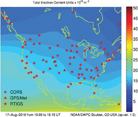
FIGURE 3.17 Example of an ionosphere map produced by the NOAA Space Weather Prediction Center August 17, 2010. The unit for total electron content (TEC) is 1016 electrons per square meter (the total number of electrons in a tube with a cross-section area of one square meter, extending vertically from the surface through the ionosphere). SOURCE: NOAA, http://www.swpc.noaa.gov/ustec/.
these biases is far more difficult in the presence of multipath error, the best way to improve knowledge of instrumental delays would be to improve multipath conditions at GNSS/GPS sites. This requires coordination on the national level to define the site requirements for infrastructure and to establish the leadership structures for implementing these requirements. The space weather community also would benefit from more sites that telemeter data in real or near-real time. The NOAA Space Weather Forecasting network now uses data from only approximately 100 real-time sites. These sites can easily assimilate more data. The United States now has more than 2,000 GPS sites supported by a variety of government agencies; however, data from these sites are often transmitted only once per day.
The Doppler Orbitography and Radiopositioning Integrated by Satellite (DORIS) system also can contribute to monitoring space weather through the launch of specially designed instruments that take advantage of worldwide DORIS transmitting beacons. The primary objective of the Scintillation and Tomography Receiver in Space (CITRIS) is to detect ionospheric irregularities from space at low latitudes. CITRIS, developed at the U.S. Naval Research Laboratory, differs from the normal DORIS receiver in that it is able to capture two-frequency transmissions at a sample rate of 200 hertz. With CITRIS flying on the U.S. Space Test Program satellite STPSat-1, two years of data were collected and processed to determine the fluctuations in ionospheric TEC and radio scintillations associated with equatorial irregularities (Bernhardt and Siefring, 2010).
PRECISION SPACECRAFT NAVIGATION
Precision Orbit Determination for Near-Earth Satellites
Over the past several decades, the requirements for highly accurate determination of the orbits of near-Earth satellites have been driven by the evolution of the fields of satellite geodesy, including reference frame and gravity field determination, satellite radar and laser altimetry, and InSAR. The ability to use accurate range and range-rate measurements between an orbiting satellite and
tracking systems located on Earth’s surface has provided a dramatic improvement in the ability to monitor tectonic deformation and subsidence as well as monitor small but important changes in Earth’s rotation. The ability to use satellite altimeter measurements to obtain accurate, globally distributed observations of the ocean surface has opened a new era in oceanography. These same tracking measurements, along with satellite-to-satellite measurements, are providing unparalleled views of Earth’s gravity field and the gravity signals associated with temporal variations in the distribution of mass within Earth. These advances are intimately tied to the advances in precision orbit determination of Earth-orbiting satellites.
Determining the orbit of near-Earth satellites involves four elements: (1) equations describing the motion of the satellite; (2) a numerical integration procedure for the equations of motion; (3) accurate observations of the satellite from the ground or other satellites; and (4) an estimation method combining the results of the first three elements to estimate the satellite’s position (Tapley and Ries, 2003). Continuous measurements of the three-dimensional position of a spacecraft are usually not available, but as long as the observations depend on the satellite’s motion, they contain information that helps to determine the orbit. The evolution of the satellite’s position and velocity must be consistent with both the physics of the mathematical model and the sequence of observations, which constrains the estimated orbit to a specific solution. As the tracking data and mathematical models for satellite dynamics have steadily improved, the accuracy of orbit determination also has improved. For example, whereas typical orbit accuracy for geodetic satellites was at the several-meter level in the 1970s, centimeter-level orbit accuracy is now achievable when high-precision tracking systems (GNSS/GPS, SLR, and/or DORIS) are used. This accuracy has been enhanced by the availability of dramatically improved Earth gravity models provided by the GRACE mission.
Interplanetary Navigation
The primary aim of interplanetary spacecraft navigation is to position spacecraft relative to solar system bodies for precise fly-bys, orbit insertion, and surface landings. This differs significantly from near-Earth orbit determination because of the difficulty in obtaining tracking, the geometry of that tracking, and the long delays in receiving signals from distant spacecraft. The data used in interplanetary spacecraft tracking are generally radiometric measurements of range, range-rate, or the interferometric difference of signal arrival times, which are provided by very large radio antennas such as those of the Deep Space Network. Optical (image) measurements also have been used, but, in recent years, these are most often performed with the imaging systems on the spacecraft as opposed to terrestrial optical telescope measurements. Interplanetary laser ranging, using transponders or one-way systems, are already being investigated, such as the current tests of one-way laser ranging to the Lunar Reconnaissance Orbit.
Like near-Earth orbit determination, the basic analysis of spacecraft-tracking data requires relating the position of the spacecraft to the position of the tracking system, but rather than orbiting Earth, an interplanetary spacecraft is orbiting the sun or some other planet. The geometry of the basic measurement of range or range-rate is not sufficient to directly determine a spacecraft’s position, but the equations of motion for the spacecraft are very accurately known. Combined with precise knowledge of the tracking station’s position, a sufficient accumulation of tracking data constrains the possible motions of the spacecraft to a particular trajectory. For this, accurate coordinates as a function of time (ephemerides) for the solar system bodies also are needed. To keep improving the planetary ephemerides, tracking data collected on spacecraft near planets are incorporated with radar and optical measurements of the planets (Standish, 1998). Another important requirement is knowledge of Earth’s orientation in space, particularly Earth’s rotation angle (denoted as Universal Time 1, or UT1, a nomenclature leftover from when time was determined by Earth’s rotation rather than atomic clocks). Wind and water movements on Earth cause UT1 variations and cannot be pre-
dicted into the future with high accuracy. Determining Earth’s orientation with real-time accuracy would require a station position equivalent of 30 centimeters, which, for UT1, requires accuracies of 650 microseconds. Current spacecraft navigation systems obtain 24-hour prediction accuracies, or 125 microseconds for UT1.
TIMING AND TIME TRANSFER
The high-accuracy timing methods at the heart of geodetic techniques are useful for precise measurements of time and frequency. The ability to synchronize distant clocks accurately is an operation commonly referred to as “time transfer.” Time synchronization requirements for such everyday functions as bank transfers, transportation, television broadcasting, and power grid regulation are on the order of milliseconds or less. GNSS/GPS signals are the most popular and economical way to achieve clock synchronization for most of these commercial applications. Scientific applications have yet more demanding time synchronization requirements, at the nanosecond level (10–9 seconds) or better. “Precise time-transfer” is typically only needed to synchronize clocks with comparable precisions (for example, atomic clocks). Because no single clock can be expected to be absolutely stable or reliable, the international definition of time for Earth (International Atomic Time or TAI) is based on an ensemble of approximately 300 atomic clocks in various laboratories around the world. Since these clocks must be compared constantly to produce the official time system, the precision of the time-transfer method is just as important as building the clocks themselves (Arias, 2005). The United States has demonstrated its long-standing commitment to the definition of TAI by contributing more than half of the clocks used to define the international timescale.
Before the advent of GNSS/GPS, the most precise method for time-transfer was TWSTFT—two-way satellite time and frequency transfer. TWSTFT used laboratory-based transponders and expensive commercial satellites with a precision of approximately 0.5–1.0 nanoseconds (Hanson, 1989). With GNSS/GPS now freely available, methods developed by the geodetic community have improved precision by a factor of 10 (Bauch et al., 2006; Larson et al., 2000). Meanwhile, kilohertz time transfer is being tested on the Jason-2 mission with the T2L2 experiment, where picosecond-level stability over several minutes may be achievable. In addition to the international timescale TAI, a few countries operate their own primary frequency standards (Arias, 2005). NIST-F1, a cesium fountain frequency standard operated by the National Institute of Standards and Technology, serves as the United States’ primary frequency standard, with an uncertainty of 5 × 10⁻¹⁶ (such a clock does not lose or gain more than one second in 60 million years). Such extraordinarily accurate clocks place the most demanding requirements for time transfer capabilities on the geodetic community and infrastructure.
DECADAL MISSIONS
The NRC’s Earth Science and Applications From Space: National Imperatives for the Next Decade and Beyond (known as the “Decadal Survey,” NRC, 2007a) recommended a number of efforts and missions to address a wide range of scientific and societal challenges, from scientific questions related to melting ice sheets and sea level change to the occurrence of extreme events like earthquakes and volcanic eruptions. Specifically, the Decadal Survey recommended three space geodetic missions: ICESat-2, DESDynI, and GRACE-II. The committee agrees with these recommendations as being of high priority to the nation. Moreover, there is an important synergy between these missions and the current geodetic infrastructure that increases the potential for scientific discovery and other societal benefits associated with these Decadal Survey missions.
As noted in the Decadal Survey, sea level will change in part due to the thermal expansion (or decrease in water density) of the oceans as a result of a global-scale increase in temperature combined with the addition of water volume from melting mountain glaciers and ice sheets. Of these factors, changes in the volume of ice sheets in response to climate change is the least understood. The laser altimeter on ICESat-2 would quantify polar ice sheet contributions to recent sea level change and illuminate the linkages to climate conditions. It also would quantify regional signatures of ice sheet changes to assess the sources of that change and to improve predictive models, as well as estimate sea ice thickness to examine how ice, the ocean, and the atmosphere exchange energy, mass, and moisture. Massive urbanization and the extensive societal and economic infrastructure that has developed in coastal areas over the past century make the precise monitoring of sea level critical. In addition, ICESat-2 would measure vegetation canopy height as a basis for estimating large-scale land biomass (the amount of living matter in a given area) and biomass changes. Land biomass stores a significant amount of carbon. Measurement of canopy height will allow scientists to better assess the effects of climate and land management on vegetation and to improve understanding of the global carbon budget.
The DESDynI (Deformation, Ecosystem Structure and Dynamics of Ice) mission would employ an L-band Synthetic Aperture Radar (SAR) and multiple-beam LiDAR to monitor surface deformation and terrestrial biomass structure. Observing surface changes is critical for estimating the likelihood of earthquakes, volcanic eruptions, and landslides, and for predicting the response of ice masses to climate change and the impact of that response on sea level. Monitoring the size and distribution of vegetation will enable characterization of the effects of changing climate and land use on species’ habitats and the global carbon budget.
The GRACE-II gravity monitoring mission, which proposes to use lasers instead of microwaves for satellite-to-satellite tracking, is expected to provide hydrological measurements down to scales approaching 100 kilometers or better (see Box 3.1). However, to avoid an undesirable gap in the gravity monitoring missions between GRACE and GRACE-II (proposed for the 2016–2020 time frame), a GRACE follow-on mission is now planned. These measurements will allow scientists to track large-scale water movement over the entire globe in order to better understand Earth’s hydrological cycle, provide inputs to meteorological models, detect changes in aquifers for improved groundwater management, and assess changes in ice sheet volume and distribution to improve predictions of sea level change.
These Decadal Survey missions are highly complementary and are essential to fully exploiting existing geodetic observation systems. For example, uncertainty in the models for how Earth’s crust accommodates changing ice load (post-glacial rebound or glacial isostatic adjustment, GIA) currently hampers the determination of changes in the Antarctic and Greenland mass balance using satellite gravity measurements. However, by combining satellite gravity measurements with satellite altimetry, it is possible to distinguish between GIA and ice mass change, because GIA-induced changes (which involve relatively dense rock) will produce a different combination of surface and gravity change than those produced by variations in ice alone. Over vegetative areas, the laser altimeter and microwave SAR instruments will monitor surface deformation at different frequencies to more precisely separate biomass changes from surface topography changes. Between the three missions, changes in mass and surface topography for nearly all of Earth’s land area will monitored for seasonal and long-term changes.
SUMMARY
The operational applications and scientific research made possible by an accurate and easily-accessible global geodetic infrastructure are limited only by the imagination of the user community. The examples presented in this chapter were selected to provide some sense of the variety
of applications in various stages of development and routine use. As the extent, density, accuracy, and accessibility of the geodetic infrastructure continues to improve, the scientific applications will continue to grow, enabling new services to be developed and new challenges to be solved.
In addition to existing systems, some “Decadal Survey” missions—DesDynI, GRACE-II, and ICESat-II—also have the potential for great direct public benefit. They will each measure, in real time, an important component of the climate system. This not only will enable scientists to gather valuable data about climate, but also will provide the public with images that will enable them to visualize the dynamic Earth system and to understand the connection and interaction among the global water cycle, climate, and the solid Earth. The Decadal Survey missions also will benefit greatly from the global geodetic infrastructure. Indeed, these missions have the potential to become part of the infrastructure by providing unique geodetic information.


