
Appendix A
Vertical Land Motion and Sea-Level Data Along the West Coast of the United States
As summarized in Chapter 4 (“Analysis of West Coast Tide Gage Records”), the committee determined rates of historical sea-level change along the California, Oregon, and Washington coasts using 12 tide gages. The rates were then corrected for vertical land motion and atmospheric pressure effects to compare sea-level rise along the west coast of the United States with the global mean sea-level rise. Details of these analyses are given below.
VERTICAL LAND MOTION FROM CONTINUOUS GPS
Tide gages are generally corrected for vertical land motions using glacial isostatic adjustment (GIA) models. However, GIA models capture only a small component of the total vertical land motion in coastal areas that are tectonically active or undergoing subsidence or uplift associated with sediment compaction and/or fluid withdrawal or recharge. The Global Positioning System (GPS) began to be used to adjust tide gage data for vertical land motion around 1997 (Ashkenazi et al., 1993; Nerem et al., 1997; Zerbini, 1997). Continuous GPS (CGPS) records along the U.S. west coast have been available since the early 1990s, although significantly more stations have been installed since 2003 as part of the National Science Foundation’s Plate Boundary Observatory.1 Continuous GPS solutions allow vertical land motions to be estimated from shorter temporal records and with more confidence than episodic sampling of the land motion signal. The committee used CGPS data to estimate and remove the vertical land motion component from the sea levels recorded by west coast tide gages. The locations of the tide gages and CGPS stations analyzed in this report are shown in Figure A.1.
Several published GPS solutions are available for estimating west coast vertical land motions, each of which uses a different number of stations, timespan, and/or processing software (e.g., Donnellan et al., 1993a,b; Dong et al., 1998; Argus et al., 1999, 2005; Bennett et al., 1999; Argus and Gordon, 2001; Spinler et al., 2010). The committee used the Scripps Orbit and Permanent Array Center (SOPAC) velocity model,2 which is a routinely updated, publicly available solution with the longest time span for each station as well as the greatest GPS station density for the U.S. west coast. The SOPAC processing details are described in Nikolaidis (2002). Briefly, GAMIT and GLOBK software (Dong et al., 1998) are used to calculate daily site positions, which are input to the velocity estimation model. Using the entire time series for a specific site, the model accounts for offsets, linear velocity, annual and semi-annual fluctuations (for stations with at least 2 years and 1 year of data, respectively), and post-seismic relaxation. Noise analysis (Williams, 2003) using white noise plus flicker noise covariances provides realistic uncertainty estimates.
A vertical land motion value was assigned to each tide gage site by taking the closest CGPS station with a velocity estimate within 15 km from the tide gage. The
__________
1 See <http://pboweb.unavco.org/>.
2 See <http://sopac.ucsd.edu/processing/refinedModelDoc.html>.
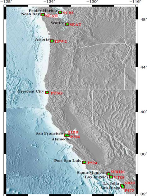
FIGURE A.1 Map showing names and locations of the 12 tide gages and CGPS stations analyzed in this report.
15-km value is somewhat arbitrary, but it is similar to the distance threshold typically used in previous joint GPS and tide gage analyses (e.g., Mazzotti et al., 2007; Wöppelmann et al., 2007). The committee’s estimated rates of vertical land motions are given in Table A.1. Positive values of vertical land motion mean that the land is rising. Table A.1 also reports the standard deviation of vertical land motion within a 15-km radius of each tide gage station. This value was used in the uncertainty estimate described below.
To test the importance of the CGPS solution on the calculated rate of vertical land motion, the committee compared the SOPAC-derived rates with rates published in the literature. Although most published reports for coastal areas south of the Mendocino Triple Junction present only horizontal rates (e.g., Spinler et al., 2010), the SOPAC rates for Cascadia are similar to vertical rates for the same sites published in Mazzotti et al. (2008). Mazzotti et al. (2008) estimated rates using different GPS processing software (BERNESE) than that used by SOPAC. The correspondence in rates produced by two independent approaches suggests that the committee’s results are reasonable.
Uncertainty in Vertical Land Motion
The estimated error in the vertical land motion adjustment to the tide gage records can be expressed as eTG = ev + esv + eref, where ev is the error in the velocity estimation, is the error associated with spatial variability in vertical land motion between a CGPS station and the tide gage, and eref is the error associated with the definition of the GPS reference frame. Of these error sources, ev is well defined (Nikolaidis, 2002; Williams et al., 2004) and is taken to be the vertical land motion error associated with the nearest CGPS station to the tide gage (and fifth and sixth columns of Table A.1).
Error in the spatial variability of vertical land motion between a CGPS station and a tide gage, esv, is locally variable and cannot be determined without more detailed studies. For example, Brooks et al. (2007) reported a variation of ~ ± 3 mm yr-1 for esv in the Los Angeles Basin. To estimate esv, the committee used the standard deviation of vertical land motion within a 15-km radius of each tide gage (right two columns in Table A.1). Using this value, rather than the formal error estimate associated with any given GPS station’s velocity, seemed justifed, given the potential for significant variability in vertical land motion at the km scale. For instance, the Santa Monica tide gage has seven CGPS stations within a 15-km radius, with vertical land motion estimates ranging from -1.5 mm yr-1 to 1.8 mm yr-1. The nearest CGPS station, WRHS, has the minimum vertical land motion estimate (-1.5 mm yr-1) and may be the most appropriate value for the correction. However, confidence in this value is diminished by the local spatial variability, which is reflected in the 15-km standard deviation value (Table A.1).
The reference frame error (eref) is a classical geodetic problem (Strang and Borre, 1997). The SOPAC
TABLE A.1 Parameters for Vertical Land Motion Correction
| Vertical Land Motion, Nearest Station |
Vertical Land Motion, 15-km Radiusa |
||||||
| Tide Gage | Nearest CGPS Station | Start Date | Distance (km) | Rate (mm yr-1) | Error (1σ) | Rate (mm yr-1) | Error (1σ) |
| Friday Harbor | SC02 | 2001.860 | 0.70 | 0.90 | 0.70 | ||
| Neah Bay | NEAH | 1996.000 | 7.71 | 3.00 | 0.40 | ||
| Seattle | SEAT | 1996.000 | 6.25 | 0.20 | 0.50 | -1.10 | 0.94 |
| Astoria | TPW2 | 2000.247 | 1.08 | 0.60 | 0.00 | 1.20 | 0.40 |
| Crescent City | PTSG | 1999.820 | 5.85 | 2.60 | 0.40 | ||
| San Francisco | TIBB | 1994.460 | 10.23 | -1.40 | 0.50 | -1.44 | 1.97 |
| Alameda | P224 | 2005.174 | 12.90 | -0.20 | 0.60 | -1.58 | 1.20 |
| Port San Luis | P524 | 2007.048 | 14.50 | 1.70 | 0.30 | ||
| Santa Monica | WRHS | 1999.770 | 9.36 | -1.50 | 0.60 | -0.01 | 1.34 |
| Los Angeles | VTIS | 1998.938 | 2.54 | -0.50 | 0.50 | -0.27 | 2.34 |
| La Jolla | SIO3 | 1993.522 | 0.26 | 2.10 | 0.50 | 0.73 | 1.11 |
| San Diego | P475 | 2007.601 | 9.17 | -3.00 | 0.20 | -4.50 | 0.81 |
a Rates and errors are not reported for 15-km areas with only 1 CGPS station.
TABLE A.2 Tide Gage Records from PSMSL, Corrected for Atmospheric Pressure and Vertical Land Motion
| Trend (mm yr-1) | Confidence Limit | Trend (mm yr-1) | |||||||
| Tide Gage | Latitude | Longitude | Period | Original Record |
With IB Adjustment |
With IB and GPS Adjustment |
Upper 95% |
Lower 95% |
With IB and GIA Adjustment |
| Friday Harbor | 48.550 | -123.000 | 1934–2008 | +1.04 | +1.14 | +2.04 | +3.44 | +0.64 | +1.31 |
| Neah Bay | 48.367 | -124.617 | 1934–2008 | -1.77 | -1.65 | +1.35 | +2.22 | +0.48 | -1.33 |
| Seattle | 47.760 | -122.333 | 1900–2008 | +2.01 | +2.10 | +2.30 | +3.29 | +1.31 | +1.67 |
| Astoria | 46.217 | -123.767 | 1925–2008 | -0.38 | -0.30 | +0.30 | +0.61 | -0.01 | -1.37 |
| Crescent City | 41.750 | -124.200 | 1933–2008 | -0.73 | -0.65 | +1.95 | +2.78 | +1.12 | -0.87 |
| San Franciscoa | 37.800 | -122.467 | 1900–2008 | +1.92 | +1.98 | +0.58 | +0.69 | +0.47 | +1.99 |
| Alameda | 37.767 | -122.300 | 1939–2008 | +0.70 | +0.82 | +0.62 | +1.82 | -0.58 | +0.85 |
| Port San Luis | 35.167 | -120.750 | 1945–2008 | +0.68 | +0.76 | +2.46 | +3.10 | +1.82 | +0.68 |
| Santa Monica | 34.017 | -118.500 | 1933–2008 | +1.41 | +1.44 | -0.09 | +0.72 | -0.90 | +1.43 |
| Los Angeles | 33.717 | -118.267 | 1923–2008 | +0.84 | +0.83 | +0.33 | +1.32 | -0.66 | +0.80 |
| La Jolla | 32.867 | -117.250 | 1924–2008 | +2.08 | +2.07 | +4.17 | +5.17 | +3.17 | +2.02 |
| San Diego | 32.717 | -117.167 | 1906–2008 | +2.04 | +2.07 | -0.96 | +0.03 | -1.95 | +2.01 |
NOTE: IB = inverse barometer.
a Although the San Francisco record starts in 1854, the IB correction starts at 1900.
velocity solution uses the International Terrestrial Reference Frame’s ITRF2005 realization,3 one of the most accurate and rigorously constrained versions of a global reference frame. ITRF2005 was developed from a combination of space geodetic observations from four independent platforms: GPS, Very Long Baseline Interferometry, Satellite Laser Ranging, and Doppler Orbit Determination and Radio-Positioning Integrated on Satellite. ITRF2005 is an improvement over previous frame realizations because it uses better antenna phase center models and its use of time series enables treatment of nonlinear and discontinuous behavior. A detailed description of the ITRF2005 realization appears in Altamimi et al. (2007).
Altamimi et al. (2007) suggested that the disagreement in origin definition between ITRF2005 and ITRF2000 (the previous frame realization) could be used as a metric of the origin accuracy. They reported a translation misfit of 0.1 mm, 0.8 mm, and 5.8 mm along the x-, y-, and z-axes, respectively, with a formal error of 0.3 mm for each component. The misfit of translation rate was reported as 0.2 mm yr-1, 0.1 mm yr-1, and 1.8 mm yr-1, with a formal error of 0.3 mm yr-1 (Altamimi et al., 2007). Mazzotti et al. (2007), using ITRF2000, estimated that their vertical land motion values could contain a reference frame bias of -0.5–0.8 mm yr-1. Given these two results and the difficulty of estimating eref in an absolute sense, the committee adopted a conservative value of ± 1 mm yr-1 for eref. The committee’s error estimates for the vertical land motion correction to the tide gages are given in Table A.2.
ANALYSIS OF SEA-LEVEL TREND FROM TIDE GAGES
Sea-level records are archived at the Permanent Service for Mean Sea Level (PSMSL).4 PSMSL reduces the data reported from each tide gage to monthly mean values and adjusts them to a common datum to produce a revised local reference dataset (Woodworth and Player, 2003). The sea-level data used in this report are all revised local reference datasets. PSMSL gives sea level in mm and, to avoid negative numbers, adds 7,000 mm to each monthly mean.
The committee examined the sea-level records from the 28 PSMSL tide gages along the west coast of the United States (Table A.2). For its analysis, the committee chose 12 tide gages that are currently operating and have records at least 60 years long. Shorter records are subject to decadal bias (Box A.1; see also “Tide Gage Measurements” in Chapter 2) and were not analyzed. Records with gaps in the data such as Santa Monica were simply treated as nonuniformly spaced in time.
__________
3 See <http://itrf.ensg.ign.fr/>.
4 See <http://psmsl.org>.
BOX A.1
Effect of Record Length on Sea-Level Trend
As noted in Chapter 2, different lengths of record yield different sea-level trends because of decadal variability. The committee investigated the effect of record length on the rate of sea-level rise by fitting a linear trend over varying lengths of record from the San Francisco tide gage. The top figure shows the trends based on a starting year of 1900 and using longer and longer record lengths. The resulting rates of sea-level rise range from 1.12 mm yr-1 to 2.10 mm yr-1. The bottom figure shows the reverse analysis, fixing the fit line at 2009 and adding progressively older data. For this case, rates of sea-level rise range from -0.05 mm yr-1 to 2.66 mm yr-1, and the recent (1980–1990) downtrend in sea level noted in Bromirski et al. (2011) can be seen. The wide range in sea-level trends depending on the starting time and the length of the record also shows the difficulty of describing a complex time-varying signal with a simple linear relationship.
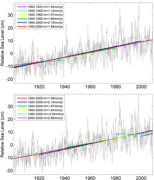
FIGURE Sea-level trends for the San Francisco tide gage data as a function of data length. (Top) Straight line fits from 1900. (Bottom) Straight line fits from 2009.
Although this approach has little or no effect on the estimated rate of sea-level rise, it slightly reduces the uncertainty (variability) when the gaps are relatively long.
The committee began the analysis of the PSMSL data by removing the 7,000 mm offset, thus reintroducing negative values. Long-term trends for the original tide gage data were obtained by fitting a straight line to the monthly average values for each record using a least squares method expressed as yt = mxt + b, where yt (in mm) is the monthly mean tide level at time xt, where t = 1, 2,…, N, and N equals the total number of observations in the record. The slope m, which represents the relative sea-level rise, is given in mm yr-1, and b is the y-intercept in mm. The linear sea-level trends (m) were determined using the entire record length of each tide gage.
Adjustments to the Original Tide Gage Trends
The committee adjusted the original tide gage trends to remove the effects of atmospheric pressure and vertical land motions, as described below.
Atmospheric Pressure
In many studies of sea-level rise, tide gage records are not adjusted for the barotropic response of the ocean due to variations in atmospheric pressure. However, observations suggest that an ocean response to atmospheric pressure loads is expected everywhere except the tropics and western boundary current extension regions (Wunsch and Stammer, 1997). The so-called inverse barometer (IB) adjustment is a good approximation of the barotropic response of sea level.
The committee adjusted the 12 tide gage records for the inverse barometer effect following the procedures of Ponte et al. (1991). The adjustment can be expressed as (P(t) - P(t)ref)/pg, where p is the density of sea water and g is the acceleration of gravity. The term -1/pg is a scale factor that converts local air pressure anomalies to water level equivalent with a value of -9.948 mm mb-1. P(t) represents the monthly averaged sea-level pressure for a specific tide gage and month at time t, and P(t)ref is the mean surface pressure taken over the global ocean for the same month. This adjustment is then subtracted from the monthly averaged sea level for that month.
Sea-level pressure data were obtained from the National Oceanic and Atmospheric Administration Earth System Research Laboratory (NOAA ESRL) 20th Century Reanalysis V2 database.5 These data are available on a 2° × 2° global grid from 1871 through 2008. The sea-level pressure for each tide gage (P(t)) was extracted from the nearest 2° × 2° box. The mean ocean surface pressure for each month (P(t)ref) was obtained by averaging over all 2° × 2° boxes. The results of the IB adjustment are shown in Table A.2. The effect of the adjustment is relatively small, changing the slope by less than 10 percent in the majority of cases. The changes appear to be smallest in southern California.
Vertical Land Motion
The tide gage records were corrected for local site motion using GPS data (see “Vertical Land Motion from Continuous GPS” above). The CGPS rates of vertical land motion were simply added to the tide gage rate of relative sea-level rise (the slope m) to obtain a new local motion-adjusted record. The GPS data extend back in time only one to two decades, while some tide gage records are more than 100 years long. For correction purposes, the committee made the crucial assumption that the GPS adjustment remains constant over the entire length of the sea-level record. This assumption is more likely valid where the vertical land motion is dominated by GIA, but it is open to question where subsidence or uplift are the primary geophysical causes. In most cases, the GPS adjustments are significantly larger than the GIA adjustments, confirming the importance of tectonics and subsidence to relative sea-level rise in the area (Table A.2).
The GPS adjustment is generally larger than the IB adjustment. The magnitude of the two adjustments varies among tide gages, with relatively large changes to the original trend in a few places due primarily to the GPS adjustment. For example, these corrections changed the slopes from -1.77 mm yr-1 to +1.35 mm yr-1 at Neah Bay, from -0.73 mm yr-1 to +1.95 mm yr-1 in Crescent City, and from +2.04 mm yr-1 to -0.96 mm yr-1 at San Diego (Table A.2). The large change at San Diego underscores the importance of small-scale spatial variability in vertical motion in the region.
__________
5 See <www.esrl.noaa.gov/psd/data/gridded/data.20thC_ReanV2.html>.
Results
Figure A.2 shows the distributions of slopes for the original tide gage data, the data with IB adjustments, and the data with IB and GPS adjustments for the 12 tide gages. The mean value of all slopes is 0.82 mm yr-1 for the original sea-level records, 0.88 mm yr-1 with the IB adjustment, and 1.25 mm yr-1 with the IB and GPS adjustments. The standard deviation increases from about 1.23 mm yr-1 to 1.39 mm yr-1 when the GPS adjustment is included. This slight increase suggests that the local variability in vertical motion is often significant and uncorrelated with the vertical motion experienced by the tide gage. It also may indicate that vertical land motions over the past one or two decades are not representative of the ground motion over the lifetime of the tide gage.
To suppress the influence of possible outliers, the slopes were plotted as a function of latitude then fit with robust or weighted lines of regression (solid red line in Figure A.3). In weighted regression, values that lie far from the line of regression are given less weight than values that lie closer to the line. The weighted regression employs iteratively reweighted least squares with a selection of weighting functions depending on what form and how much weighting is desired (Holland and Welsch, 1977). The form of weighting chosen was the Welsch weight function. The weights, w(r), are given by exp (-r2), where r is related to the distance between a given value and the line of regression. For a more detailed explanation, see Huber (1981). The process for deciding what weighting to use is somewhat subjective, but tests using several different weight functions did not significantly affect the results. The calculated slopes seldom varied by more than ± 10 percent.
To examine the variation in sea-level trends along the coastline, a weighted regression was applied to all 12 gages. The linear trend in the weighted regression for the entire coast shows a significant increase in slope from south to north (Figure A.3, solid red line), whereas the original data (dashed red line) show a decrease from south to north. The change in trend reflects vertical land motion along the coast.
Uncertainty in Adjusted Sea-Level Trends
The 95 percent confidence limits in the sea-level trends were calculated using measures of uncertainty for the original records and the GPS adjustments. For data where the individual observations are statistically independent, confidence limits are calculated using the student’s t distribution. However, with time series, the observations are generally not independent, so the equivalent number of independent observations or degrees-of-freedom (DOFs) is often far less than the total number of observations in the original time series. For DOFs greater than 120, the t values do not change and no adjustment for serial correlation is required.
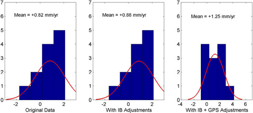
FIGURE A.2 Distributions of slopes for the original relative sea-level data (left), with inverse barometer (IB) corrections (center), and with IB plus GPS corrections (right).

FIGURE A.3 Slopes of linear trends for tide gage records and weighted lines of regression. Slopes for original tide gage records (stars), for IB adjusted records (+), and for IB and GPS adjusted records (o) are shown as a function of latitude from north to south, together with weighted linear trends for the entire coast for the original data (dotted red line) and for the GPS-adjusted data (solid red line).
Several approaches are used to estimate the DOFs when the data are serially correlated, as they are in this case. The committee used the Mitchell et al. (1966) approach to calculate the DOFs for each record, and found that the DOFs were greater than 120 in all cases. Calculating the 95 percent confidence limits reduces to the slope ± 1.96 (from the t table) times the square root of the estimated variance of the trend. The confidence interval is thus equal to the difference between the upper and lower confidence limits.
Estimating the confidence limits for the GPS-adjusted trends requires not only a measure of uncertainty associated with the tide gage records but also a measure of uncertainty associated with the GPS data, in this case, the standard deviations. Assuming that the uncertainties for the slopes of the tidal records and the GPS data are independent, the combined uncertainty is equal to the square root of the sum of the variances associated with each. Multiplying this value by 1.96 yields the 95 percent confidence limits. The upper and lower confidence limits are included in Table A.2. In some cases, the uncertainties associated with the GPS data far exceed those associated with the tide gage data.
REFERENCES
Altamimi, Z., X. Collilieux, J. Legrand, B. Garayt, and C. Boucher, 2007, ITRF2005: A new release of the International Terrestrial Reference Frame based on time series of station positions and Earth orientation parameters, Journal of Geophysical Research, 112, B09401, doi:10.1029/2007JB004949.
Argus, D.F., and R.G. Gordon, 2001, Present tectonic motion across the Coast Ranges and San Andreas Fault System in central California, Geological Society of America Bulletin, 113, 1580-1592.
Argus, D.F., M.B. Heflin, A. Donnellan, F.H. Webb, D. Dong, K.J. Hurst, D.C. Jefferson, G.A. Lyzenga, M.M. Watkins, and J.F. Zumberge, 1999, Shortening and thickening of metropolitan Los Angeles measured and inferred by using geodesy, Geology, 27, 703-706.
Argus, D.F., M.B. Heflin, G. Peltzer, F. Crampe, and F.H. Webb, 2005, Interseismic strain accumulation and anthropogenic motion in metropolitan Los Angeles, Journal of Geophysical Research, 110, B04401, doi:10.1029/2003JB002934.
Ashkenazi, V., R.M. Bingley, G.M. Whitmore, and T.F. Baker, 1993, Monitoring changes in mean sea-level to millimetres using GPS, Geophysical Research Letters, 20, 1951-1954.
Bennett, R.A., J.L. Davis, and B.P. Wernicke, 1999, Present-day pattern of Cordilleran deformation in the western United States, Geology, 27, 371-374.
Bromirski, P.D., A.J. Miller, R.E. Flick, and G. Auad, 2011, Dynamical suppression of sea level rise along the Pacific Coast of North America: Indications for imminent acceleration, Journal of Geophysical Research, 116, C07005, doi:10.1029/2010JC006759.
Brooks, B.A., M.A. Merrifield, J. Foster, C.L. Werner, F. Gomez, M. Bevis, and S. Gill, 2007, Space geodetic determination of spatial variability in relative sea level change, Los Angeles Basin, Geophysical Research Letters, 34, L01611, doi:10.1029/2006GL028171.
Dong, D., T.A. Herring, and R.W. King, 1998, Estimating regional deformation from a combination of space and terrestrial geodetic data, Journal of Geodesy, 72, 200-214.
Donnellan, A., B.H. Hager, and R.W. King, 1993a, Discrepancy between geological and geodetic deformation rates in the Ventura Basin, Nature, 366, 333-336.
Donnellan, A., B. Hager, R. King, and T. Herring, 1993b, Geodetic measurement of deformation in the Ventura Basin region, southern California, Journal of Geophysical Research, 98, 21,727-21,739.
Holland, P.W., and R.E. Welsch, 1977, Robust regression using iteratively reweighted least-squares, Communications in Statistics: Theory and Methods, A6, 813-827.
Huber, P.J., 1981, Robust Statistics, John Wiley & Sons, New York, 308 pp.
Mazzotti, S., A. Lambert, N. Courtier, L. Nykolaishen, and H. Dragert, 2007, Crustal uplift and sea level rise in northern Cascadia from GPS, absolute gravity, and tide gauge data, Geophysical Research Letters, 34, L15306, doi:10.1029/2007GL030283.
Mazzotti, S., C. Jones, and R.E. Thomson, 2008, Relative and absolute sea level rise in western Canada and northwestern United States from a combined tide gauge-GPS analysis, Journal of Geophysical Research, 113, C11019, doi:10.1029/2008JC004835.
Mitchell, Jr., J.M., B. Dzerdzeevskii, H. Flohn, W.L. Hofmeyr, H.H. Lamb, K.N. Rao, and C.C. Walléen, 1966, Climate Change, Report of a working group of the Commission for Climatology, Technical Note 79, World Meteorological Organization, WMO No. 195, Geneva, Switzerland, 79 pp.
Nerem, R.S., T.M. van Dam, and M.S. Schenewerk, 1997, A GPS network for monitoring absolute sea-level in the Chesapeake Bay: BAYONET, in Proceedings of the Workshop on Methods for Monitoring Sea Level: GPS and Tide Gauge Benchmark Monitoring and Altimeter Calibration, Jet Propulsion Laboratory Publication 97-017, Pasadena, CA, pp. 107-115.
Nikolaidis, R., 2002, Observation of Geodetic and Seismic Deformation with the Global Positioning System, Ph.D Thesis, University of California, San Diego, 249 pp.
Ponte, R.M., D.A. Salstein, and R.D. Rosen, 1991, Sea level response to pressure forcing in a barotropic numerical model, Journal of Physical Oceanography, 21, 1043-1957.
Spinler, J.C., R.A. Bennett, M.L. Anderson, S.F. McGill, S. Hreinsdóttir, and A. McCallister, 2010, Present-day strain accumulation and slip rates associated with southern San Andreas and eastern California shear zone faults from GPS, Journal of Geophysical Research, 115, B11407, doi:10.1029/2010JB007424.
Strang, G., and K. Borre, 1997, Linear Algebra, Geodesy, and GPS, Wellesley-Cambridge Press, Wellesley, MA, 624 pp.
Williams, S.D.P., 2003, The effect of coloured noise on the uncertainties of rates estimated from geodetic time series, Journal of Geodesy, 76, 483-494.
Williams, S.D.P., Y. Bock, P. Fang, P. Jamason, R.M. Nikolaidis, L. Prawirodirdjo, M. Miller, and D.J. Johnson, 2004, Error analysis of continuous GPS position time series, Journal of Geophysical Research, 109, B03412, doi:10.1029/2003JB002741.
Woodworth, P.L., and R. Player, 2003, The permanent service for mean sea level: An update to the 21st century, Journal of Coastal Research, 19, 287-295.
Wöppelmann, G., B.M. Miguez, M.N. Bouin, and Z. Altamimi, 2007, Geocentric sea-level trend estimates from GPS analyses at relevant tide gauges world-wide, Global Planetary Change, 57, 396-406.
Wunsch, C., and D. Stammer, 1997, Atmospheric loading and the oceanic “inverted barometer” effect, Reviews of Geophysics, 35, 79-107.
Zerbini, S., 1997, The SELF II project, in Proceedings of the Workshop on Methods for Monitoring Sea Level: GPS and Tide Gauge Benchmark Monitoring and Altimeter Calibration, Jet Propulsion Laboratory Publication 97-017, Pasadena, CA, pp. 93-95.
This page intentionally left blank.


