
Appendix E
Cryosphere Extrapolations
EXTRAPOLATION BY GENERALIZED LINEAR MODEL
Extrapolations into the future, based on observational records, were done separately for the three categories of ice sources (glaciers and ice caps, Greenland Ice Sheet, and Antarctic Ice Sheet) using a generalized linear model (GLM) approach. The data were assumed to have a normal distribution, and the parameters of the model were estimated using a weighted least squares approach, which allows data uncertainty to be incorporated (McCullagh and Nelder, 1989). This is especially important because there are multiple data sets for each category with different estimates of data error. Traditionally, the data uncertainty is discarded in fitting the models, thus exaggerating the trends in the face of uncertain information.
For each data set in a category, the weighted least squares method was applied to obtain a robust linear model. The linear model is
Y = Xβ + ε,
where Y is the vector of response variable (ice mass loss rate per year), X is the matrix of the dependent variables (in this case, the intercept represented as a column of 1 and year), β is the vector of model coefficients (in this case β0 and β1), Xβ is the model estimate (Ŷ), and ε is the error assumed to be normally distributed with mean zero and variance σ2. Using weighted least squares, β is estimated as
β = (XT W X)-1(XT W Y).
Here W is a diagonal matrix containing the uncertainty of each observation. It is populated as 1/di, where di is the error associated with each observation point i.
The variance of the error is obtained from standard linear model theory (McCullagh and Nelder, 1989):
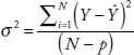
where N is the number of observations used in the model fitting and p is the number of model coefficients.
With the fitted model, estimate of the response variable for any time i is obtained as Ŷi=Xiβ, and the 95 percent prediction interval (or prediction uncertainty) is obtained as
![]()
It is apparent from the above equation that the intervals tend to widen as the extrapolation domain extends further from the observations. The term within the curly bracket is the standard error of the estimate Ŷi.
Multi-Data Averaging
Several independent data sets are available for loss rates from glaciers and ice caps as well as for the Greenland and Antarctic ice sheets (data sources are described below). The following steps were performed to obtain a multi-data averaged estimate and standard error for each category of ice source. First, a weighted least squares based linear model was fit for each data set for a given category of ice source c following the
method described above. Second, the multiple estimates were combined using a weighted averaging approach in which each estimate was weighted according to its standard error. In the following discussion, the subscript ic refers to a variable within category c at time i. Suppose that, for a category, K data sets are available; thus, for any year i in the future, K estimates Ŷij, j = 1,2, --- K can be obtained along with their standard errors eij, j = 1,2, --- K. A normalized set of weights is computed as
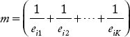
and
![]()
for j = 1,2…K. The weighted estimate is obtained as
![]()
and its standard error as
![]()
The 95 percent confidence interval of this weighted estimate is provided as
![]()
These calculations were applied for each of the three ice categories, yielding a multi-data averaged estimate and standard error for each.
Third, the global ice mass loss rate for any year i and error were calculated. The global ice mass loss rate was estimated as
![]()
and the standard error as
![]()
The 95 percent confidence interval of this multi-data averaged global mass loss rate is
![]()
The second and third steps were repeated for all of the projection years. The mass loss rates and the interval were subsequently converted to sea-level rates and then cumulatively summed.
RAPID DYNAMIC RESPONSE
Simple extrapolation of existing trends will not capture the effect of rapid dynamic response that begins after the period of observation. The committee calculated the effects of both acceleration and deceleration in ice discharge relative to observed present-day rates, as described below. The term “rapid dynamic response” is defined here as mass changes in a glacier or ice sheet that occur at rates faster than accompanying climatic mass balance and which force glacier or ice sheet conditions further away from equilibrium with climate.
Increases in Dynamic Discharge
To simulate the effect of rapid dynamics, supplementary ice fluxes were added to the loss rates determined by extrapolation. The parameters for the added rapid dynamic response are summarized in Box E.1. The choice of dynamic variations was intended to capture the general magnitude of plausible changes. Although these particular events may not occur, the calculations provide a means to quantitatively estimate the influence of rapid dynamic response on sea-level rise and to translate ranges of plausible future glaciological changes into equivalent sea-level changes.
The range of added rapid dynamic response for each ice source for each projection period is given in Table E.1, and the effect of the simulated rapid dynamic response on the projections, summed for all three sources, is shown in Table E.2. The top rows (“base values”) of Table E.2 show the integrated cumulative sea-level rise from the extrapolation and the low and high values based on uncertainties in the extrapolation. The middle rows of Table E.2 show the effect of additional rapid dynamic response on the projections of sea-level rise. The bottom rows (“percentage effect”) in Table E.2 show the effect of added dynamics expressed as a percentage of total sea-level rise. Rapid dynamic response is not an insignificant factor in future sea-level rise, but according to this simple analysis, it is also not a “wild card” variable that will swamp all other sources if it comes into play.
BOX E.1
Parameters for Added Rapid Dynamic Response
Added dynamics (additional discharge assigned to each land ice source for simulation of increased rapid dynamic contribution)
• Glaciers and ice caps: 50 percent of 324.8 GT yr-1 = 162.4 GT yr-1
• Greenland Ice Sheet: Increase outlet glacier speed by 2 km yr-1 = 375.1 GT yr-1
• Antarctic Ice Sheet: Double outlet glacier discharge to 264 GT yr-1
Variations (perturbations to base values selected for discharge used in the sensitivity calculation)
• Glaciers and ice caps: Use 30 percent and 70 percent of 324.8 GT yr-1
• Greenland Ice Sheet: Use 80 percent and 120 percent of 375.1 GT yr-1
• Antarctic Ice Sheet: Use 80 percent and 120 percent of 264 GT yr-1
TABLE E.1 Range of Added Rapid Dynamic Response (cm) for the Cryosphere Components of Sea-Level Rise
| Term | 2030 | 2050 | 2100 |
| Glaciers and ice caps | 0–0.5 | 0–1.4 | 0–3.7 |
| Greenland | 0–1.2 | 0–3.3 | 0–8.4 |
| Antarctica | 0–0.8 | 0–2.3 | 0–5.9 |
| Total cryosphere | 0–2.5 | 0–7.0 | 0–18.0 |
TABLE E.2 Effect of Rapid Dynamic Response and Uncertainty on Future Cumulative Sea-Level Rise
| 2030 | 2050 | 2100 | |
| Base values: Projected sea-level rise Z with uncertainty δZ (cm) | |||
| Z Z - δ Z Z + δ Z |
6.6 5.9 7.3 |
17.7 14.1 19.0 |
57.0 44.2 69.6 |
| Projected sea-level rise with added dynamics Zd (cm) | |||
| Zd Z + Zd Z - δ Z + Zd Z + δ Z + Zd |
2.5 9.1 8.4 9.8 |
7.0 24.7 21.1 26.0 |
18.0 75.0 62.2 87.6 |
| Percentage effect of added dynamics | |||
| Z + Zd Z - δ Z + Zd Z + δ Z + Zd |
38% 42% 34% |
40% 50% 37% |
32% 41% 26% |
Sensitivity of the Added Dynamics Analysis
The choice of fluxes for added rapid dynamic response (Box E.1) was guided by the analogy to the doubling of the Greenland mass balance deficit in 2000–2006 but was otherwise rather arbitrary. To investigate how sensitive this calculation is to the choice of added discharge flux, the input variables (discharge from glaciers and ice caps, Greenland, and Antarctica) were varied by ± 20 percent individually (no two inputs were varied at the same time), and the calculation was repeated to determine the response in the output (additional sea-level rise). The result of this sensitivity test is summarized in Table E.3. For variations of 20 percent magnitude in the inputs, output magnitudes varied by no more than 7 percent.
TABLE E.3 Sensitivity of Rapid Dynamic Response Estimate to the Choice of Parameters
| Percentage Change | Δ mm Sea-Level Rise | |
| Glaciers and ice caps | ||
| 30 percent of 324.8 GT yr-1 | 0.99 | 179 |
| 70 percent of 324.8 GT yr-1 | 1.01 | 182 |
| Greenland Ice Sheet | ||
| 80 percent of 375.1 GT yr-1 | 0.9 | 165 |
| 120 percent of 375.1 GT yr-1 | 1.09 | 197 |
| Antarctic Ice Sheet | ||
| 80 percent of 264 GT yr-1 | 0.93 | 169 |
| 120 percent of 264 GT yr-1 | 1.07 | 192 |
NOTE: Input parameters were varied by ± 20 percent individually (only one parameter was varied at a time).
TABLE E.4 Effect of Reduced Greenland Dynamic Discharge on Sea-Level Rise Projections
| Year | Total Sea-Level Rise (mm) | Cryosphere Component (mm) |
| Base-Rate Projection (From Table 5.2) | ||
| 2030 | 135 | 81 |
| 2050 | 280 | 180 |
| 2100 | 827 | 584 |
| 50 Percent Slowdown in Greenland Dynamic Discharge | ||
| 2030 | 128 | 76 |
| 2050 | 273 | 168 |
| 2100 | 774 | 535 |
| Percent Change | ||
| 2030 | -5% | -6% |
| 2050 | -3% | -7% |
| 2100 | -6% | -8% |
Decreases in Dynamic Discharge
To test the effect of decreased dynamic discharge, the projected output of the Greenland Ice Sheet was reduced by 25 percent from its projected base value and all other cryosphere terms were left unchanged. The results are summarized in Table E.4. The table shows the cumulative sea-level rise (central value only) for 2030, 2050, and 2100 for both the base rate projection (Table 5.2) and for a 50 percent reduction in Greenland calving discharge (equivalent to a 25 percent reduction in overall Greenland discharge). The cryosphere component totals are for the Greenland and Antarctica ice sheets, glaciers, and ice caps, and the total sea-level rise includes the steric component. The percent change rows show that reducing the Greenland discharge affects sea-level projections by a maximum of 8 percent.
EFFECT OF SEA-LEVEL FINGERPRINT
The influence of melting from Alaska, Greenland, and Antarctica on regional sea level was described in “Sea-Level Fingerprints of Modern Land Ice Change” in Chapter 4. To estimate this effect on projected future sea-level rise, land ice loss rates were subdivided into Alaska, Greenland, Antarctic, and all other glacier and ice cap losses other than Alaska. The fingerprint scale factors for Alaska, Greenland, and Antarctica (specified in Table 4.1) were then applied to losses from those regions, on a year-by-year basis, and the losses from other glacier and ice cap regions were carried forward without adjustment. The projected sea level ΔZ at destination region p and time t is then, using the notation defined in Appendix C:
![]()
where R is rate of ice loss (e.g., in GT yr-1), s is the fingerprint scale factor, k =1,2,3 is the set of source locations (Alaska, Greenland, and Antarctica), p = 1,2,3 is the set of destination locations (north coast, central coast, south coast), and t is time. The term RGIC-AK designates the loss rate from all glacier and ice cap regions with the exception of Alaska.
REFERENCE
McCullagh, P., and J.A. Nelder, 1989, Generalized Linear Models, 2nd edition, Chapman and Hall, London, 532 pp.
This page intentionally left blank.


