
Additional Information About the Panel’s Analyses
This appendix provides additional information about and results from the analyses conducted by the panel, as described in Chapter 4. Included are three parts. The first complements the comparisons discussed in Chapter 4 with some additional tables concerning the differences between American Community Survey (ACS) estimates and administrative estimates based on the National Center for Education Statistics’(NCES) Common Core of Data (CCD). The second part describes the model used to assess stability over time and provides detailed model results. The third part describes the panel’s exploration of the use of global regression models for predicting differences between ACS and CCD estimates for the blended reimbursement rate (BRR) using a variety of covariates from the CCD.
PART 1: COMPARISONS OF ACS ESTIMATES AND ESTIMATES BASED ON ADMINISTRATIVE DATA
Tables F-1 and F-2 display the differences between ACS multiyear averages and CCD multiyear averages computed over roughly the same time periods. Table F-1 displays comparisons for 5-year estimates and Table F-2 for 3-year estimates. These tables present differences by district size (small, medium, and large), and free or reduced-price lunch (FRPL) category (very high, high, and low to moderate) for percentage eligible for free meals, percentage eligible for reduced-price meals, percentage eligible for free or reduced-price meals, and the BRR.
TABLE F-1 Average Differences Between ACS 5-Year Estimates and 5-Year Averages of CCD Estimates
| Estimand | All Districts | Large Districts | Medium Districts | Small Districts |
| Very High FRPL Districts | (1,435) | (113) | (207) | (1,115) |
| Percentage free | –17.7 | –15.2 | –17.3 | –18.0 |
| Percentage reduced price | 3.2 | 3.6 | 4.1 | 3.0 |
| Percentage free or reduced price | –14.5 | –11.7 | –13.2 | –15.0 |
| BRR, $ | –0.35 | –0.29 | –0.32 | –0.36 |
| High FRPL Districts | (3,782) | (280) | (628) | (2,874) |
| Percentage free | –6.5 | –8.8 | –7.3 | –6.2 |
| Percentage reduced price | 1.9 | 2.2 | 2.3 | 1.8 |
| Percentage free or reduced price | –4.7 | –6.6 | –5.0 | –4.4 |
| BRR, $ | –0.12 | –0.16 | –0.13 | –0.11 |
| Low to Moderate FRPL Districts | (3,634) | (263) | (553) | (2,818) |
| Percentage free | –1.4 | –3.7 | –2.9 | –9.4 |
| Percentage reduced price | 2.3 | 2.0 | 1.9 | 2.4 |
| Percentage free or reduced price | 0.8 | –1.7 | –1.0 | 1.4 |
| BRR, $ | 0.01 | –0.05 | –0.03 | 0.02 |
NOTES: The ACS 5-year estimates (for 2005-2009) are compared with the average of CCD estimates for 2005-2006, 2006-2007, 2007-2008, 2008-2009, and 2009-2010. ACS = American Community Survey; BRR = blended reimbursement rate; CCD = Common Core of Data; FPRL = free or reduced-price lunch.
SOURCE: Prepared by the panel.
The purpose of this comparison is to illustrate the differences that exist when the reference periods of the ACS and administrative estimates are as similar as possible. These tables display the same patterns as those observed in Chapter 4, where the administrative estimates pertain to the most recent year of the reference period for the ACS estimates. Namely, the ACS understates percentage free, percentage free or reduced price, and the BRR and overstates percentage reduced price. The differences are substantial in very high FRPL districts and are least pronounced in low to moderate FRPL districts; high FRPL districts fall in between. Over all districts, the BRR is understated by the 5-year ACS by 35 cents for very high FRPL districts and 12 cents for high FRPL districts, and is overstated by 1 cent in low to moderate FRPL districts.
Chapter 4 highlights the systematic differences between ACS and CCD estimates for eligibility percentages and the BRR. The following tables compare enrollment estimates from the two sources. Tables F-3 and F-4 illustrate the differences between ACS multiyear estimates and CCD
TABLE F-2 Average Differences Between ACS 3-Year Estimates and 3-Year Averages of CCD Estimates
| Large and Medium Districts | |||
| Estimand | 2005-2007 | 2006-2008 | 2007-2009 |
| Very High FRPL Districts | (327) | (333) | (329) |
| Percentage free | –17.1 | –17.6 | –17.6 |
| Percentage reduced price | 3.5 | 2.9 | 3.2 |
| Percentage free or reduced price | –13.6 | –14.7 | –14.4 |
| BRR, $ | –0.33 | –0.35 | –0.35 |
| High FRPL Districts | (918) | (964) | (962) |
| Percentage free | –7.5 | –8.7 | –9.5 |
| Percentage reduced price | 1.9 | 1.7 | 1.9 |
| Percentage free or reduced price | –5.6 | –7.0 | –7.6 |
| BRR, $ | –0.14 | –0.17 | –0.19 |
| Low to Moderate FRPL Districts | (830) | (916) | (973) |
| Percentage free | –2.8 | –3.5 | –4.1 |
| Percentage reduced price | 1.6 | 1.3 | 1.3 |
| Percentage free or reduced price | –1.2 | –2.2 | –2.9 |
| BRR, $ | –0.03 | –0.06 | –0.07 |
NOTES: The ACS 3-year estimates are compared with 3-year averages of CCD estimates. For example, the ACS estimates for 2005-2007 are compared with the average of CCD estimates for 2005-2006, 2006-2007, and 2007-2008. ACS = American Community Survey; BRR = blended reimbursement rate; CCD = Common Core of Data; FPRL = free or reduced-price lunch.
SOURCE: Prepared by the panel.
multiyear average estimates computed over the same time periods as the ACS estimates, as well as the differences between the ACS multiyear estimates and the CCD estimates for the most recent school year that overlaps the ACS reference period. (For the latter, the ACS estimate for 2005-2009 is compared with the CCD estimate for 2009-2010, and the ACS estimate for 2007-2009 is also compared with the CCD estimate for 2009-2010.)
In addition to sampling error in the ACS estimates and various other errors in both the ACS and administrative estimates, enrollment estimates may differ because school district boundaries are different in different years. All of the ACS estimates are based on the school district boundaries recorded in the Census Bureau’s Topologically Integrated Geographic Encoding and Referencing (TIGER) database for 2009-2010 and data reflecting the number of students that resided within those boundaries at some time during a calendar year. On the other hand, the CCD data reflect the district’s enrollment as of October of a school year based on the boundaries for that year. School choice is another reason why enrollment estimates may differ. Children who live in the catchment area of a school
| Large Districts | Medium Districts | |||||
| 2005-2007 | 2006-2008 | 2007-2009 | 2005-2007 | 2006-2008 | 2007-2009 | |
| (118) | (119) | (116) | (209) | (214) | (213) | |
| –15.1 | –16.4 | –16.8 | –18.2 | –18.3 | –18.1 | |
| 3.6 | 2.8 | 3.0 | 3.4 | 3.0 | 3.4 | |
| –11.5 | –13.6 | –13.8 | –14.7 | –15.3 | –14.7 | |
| –0.28 | –0.33 | –0.33 | –0.36 | –0.37 | –0.36 | |
| (286) | (293) | (292) | (632) | (671) | (670) | |
| –8.9 | –9.8 | –10.4 | –7.0 | –8.2 | –9.2 | |
| 2.1 | 1.7 | 1.8 | 1.9 | 1.7 | 1.9 | |
| –6.8 | –8.2 | –8.6 | –5.1 | –6.5 | –7.2 | |
| –0.17 | –0.20 | –0.21 | –0.13 | –0.16 | –0.18 | |
| (270) | (293) | (303) | (560) | (623) | (670) | |
| –3.3 | –4.3 | –4.7 | –2.6 | –3.1 | –3.9 | |
| 1.8 | 1.3 | 1.4 | 1.6 | 1.3 | 1.2 | |
| –1.4 | –3.0 | –3.2 | –1.0 | –1.8 | –2.7 | |
| –0.04 | –0.08 | –0.08 | –0.03 | –0.08 | –0.07 | |
district and attend public school may not attend a school associated with the local public school district; some may attend an independent charter school, for example. These differences are discussed more fully in Chapter 4. Differences in the inclusion of prekindergarten students might also contribute to differences in enrollment estimates.
The differences shown in Table F-3 for the 5-year ACS estimates tend to be relatively small, but are largest (11 percent) for large very high FRPL districts (when compared with CCD estimates for 2009-2010). Other categories of districts have differences of 4 percent or less. The 5-year ACS estimates tend to overstate enrollment in very high FRPL districts and to understate enrollment in low to moderate FRPL districts. Similar patterns are illustrated in Table F-4, where small districts are not included because there are no 3-year ACS estimates for them.
Table F-5 shows the average differences between ACS 1-year estimates for enrollment and the CCD estimates for enrollment for each of 5 years. The ACS calendar-year estimates are compared with the CCD school year estimates for the most recent school year that overlaps the
TABLE F-3 Average Differences Between ACS 5-Year Estimates of Enrollment and Various CCD Estimates
| Estimand | All Districts |
Large Districts |
Medium Districts |
Small Districts |
| Very High FRPL Districts | ||||
| Difference from CCD for 09-10 | 358 | 4,038 | 233 | 33 |
| As percentage of 09-10 CCD | 9 | 11 | 4 | 4 |
| Difference from CCD 5-year average | 248 | 2,787 | 175 | 5 |
| As percentage of CCD 5-year average | 6 | 7 | 3 | 1 |
| High FRPL Districts | ||||
| Difference from CCD for 09-10 | –25 | –19 | –27 | –26 |
| As percentage of 09-10 CCD | –1 | 0 | 0 | –3 |
| Difference from CCD 5-year average | –47 | –188 | –32 | –36 |
| As percentage of CCD 5-year average | –1 | –1 | –1 | –4 |
| Low to Moderate FRPL Districts | ||||
| Difference from CCD for 09-10 | –124 | –1,040 | –192 | –30 |
| As percentage of 09-10 CCD | –4 | –4 | –4 | –3 |
| Difference from CCD 5-year average | –112 | –647 | –161 | –53 |
| As percentage of CCD 5-year average | –3 | –3 | –3 | –5 |
NOTES: The ACS 5-year estimates are compared with (1) CCD estimates for the most recent school year that overlaps the reference period of the ACS estimates (so the ACS estimates for 2005-2009 are compared with CCD estimates for 2009-2010) and (2) 5-year averages of CCD estimates (so the ACS estimates for 2005-2009 are compared with the average of CCD estimates for 2005-2006, 2006-2007, 2007-2008, 2008-2009, and 2009-2010). ACS = American Community Survey; CCD = Common Core of Data; FPRL = free or reduced-price lunch.
SOURCE: Prepared by the panel.
calendar year. (Hence, the ACS estimate for 2009 is compared with the CCD estimate for 2009-2010.) These results are only for large districts that have ACS 1-year estimates. The percentage differences are again largest for the very high FRPL districts (averaging almost 10 percent) and lowest for the low to moderate FRPL districts (averaging about 5 percent); the high FRPL districts average –.3 percent. Here the average differences appear to be increasing in magnitude over time for both the very high and low to moderate FRPL categories.
Tables F-6 through F-8 display the average differences between various ACS estimates (5-year, 3-year, and 1-year) and the CCD estimate for the most recent school year that overlaps the reference period of the ACS estimate for low to moderate FRPL districts. These tables complement Tables 4-1, 4-2, and 4-3 in Chapter 4, which present results for the very high and high FRPL districts. Each table shows average differences for percentage free, percentage reduced price, percentage free or reduced price, and the BRR. Tables F-6, F-7, and F-8 show the same patterns of differences
as the tables in Chapter 4, but the magnitudes of the differences are much smaller.
Let Adt denote the 1-year ACS estimate of the true BRR, Cdt, for school district d in year t, where Cdt is the BRR value as computed from the CCD.1 We write
Cdt = µt + Md + mdt
where µt is a common time trend across districts, Md is a district-specific deviation that is constant over time, and mdt is the district- and time-specific deviation from the common time trend and constant district deviation. We write
Adt = Cdt + βt + Bd + bdt + edt
where edt is sampling error with known variance σ2dt, and βt + Bd + bdt represents the difference between the CCD and ACS estimates after sampling error is removed. Because the CCD is treated as the gold standard in this discussion, we refer to βt + Bd + bdt as “bias,” with βt representing a common time trend in the bias across districts, Bd representing a district-specific bias that is constant over time, and bdt representing the district- and time- specific deviation from the common time trend and constant district-specific bias. Biases here are due primarily to measurement error from the use of different concepts and measurements between the ACS and the CCD.
We treat μt and βt as fixed effects (nonrandom) and the remaining terms as random effects. Hence, Md, mdt, Bd, bdt, and edt are assumed to be zero mean random processes, with the following conditions on the theoretical variances and covariances:
- Md and Bd are correlated with each other but uncorrelated with mdt and gdt = bdt + edt.
- Both mdt and gdt are first-order autoregressive (AR(1)) processes, and their correlation with each other also has AR(1) form. All three AR(1) models have the same autoregressive coefficient.2
____________
1 As discussed in Chapters 2-4, administrative estimates are also subject to error.
2 In SAS, this is called the UN@AR(1) covariance structure. Although preliminary investigations did indicate similar, weak correlations for mdt and gdt and weak cross-correlations, the assumption of common autoregressive parameters is primarily for simplicity. In particular, it allows use of a built-in covariance structure, UN@AR(1), in SAS Proc Mixed.
TABLE F-4 Average Differences Between ACS 3-Year Estimates of Enrollment and Various CCD Estimates
| Estimand | Large and Medium Districts | |||
| 2005-2007 | 2006-2008 | 2007-2009 | ||
| Very High FRPL | ||||
| Difference from CCD for 1 SY | 1,438 | 1,529 | 1,276 | |
| As percentage of 1-year CCD | 7 | 8 | 8 | |
| Difference from CCD 3-year average | 1,183 | 1,290 | 1,013 | |
| As percentage of CCD 3-year average | 6 | 7 | 6 | |
| High FRPL Districts | ||||
| Difference from CCD for 1 SY | –133 | –13 | –13 | |
| As percentage of 1-year CCD | –1 | 0 | 0 | |
| Difference from CCD 3-year average | –118 | –85 | –80 | |
| As percentage of CCD 3-year average | –1 | –1 | –1 | |
| Low to Moderate FRPL Districts | ||||
| Difference from CCD for 1 SY | –484 | –383 | –439 | |
| As percentage of 1-year CCD | –4 | –3 | –4 | |
| Difference from CCD 3-year average | –347 | –371 | –428 | |
| As percentage of CCD 3-year average | –3 | –3 | –4 | |
NOTES: The ACS 3-year estimates are compared with (1) CCD estimates for the most recent school year that overlaps the reference period of the ACS estimates (so ACS estimates for 2005-2007 are compared with CCD estimates for 2007-2008) and (2) 3-year averages of CCD estimates (so ACS estimates for 2005-2007 are compared with the average of CCD estimates
TABLE F-5 Average Differences Between ACS 1-Year Estimates of Enrollment and CCD Estimates
| Estimand | 2005 | 2006 | 2007 | 2008 | 2009 |
| Very High FRPL Districts | |||||
| Difference from CCD | 3,149 | 3,941 | 4,628 | 5,057 | 4,418 |
| As percentage of CCD | 7 | 9 | 10 | 11 | 12 |
| High FRPL Districts | |||||
| Difference from CCD | –184 | –211 | –297 | –111 | –131 |
| As percentage of CCD | –1 | –1 | –1 | 0 | 0 |
| Low to Moderate FRPL | |||||
| Districts | |||||
| Difference from CCD | –767 | –1,295 | –1,554 | –1,650 | –1,839 |
| As percentage of CCD | –3 | –5 | –6 | –6 | –7 |
NOTES: Calendar year ACS estimates are compared with the CCD estimates for the most recent school year that overlaps the calendar year of the ACS. For example, the ACS estimates for 2009 are compared with the CCD estimates for 2009-2010. ACS = American Community Survey; CCD = Common Core of Data; FPRL = free or reduced-price lunch.
SOURCE: Prepared by the panel.
| Large Districts | Medium Districts | |||||
| 2005-2007 | 2006-2008 | 2007-2009 | 2005-2007 | 2006-2008 | 2007-2009 | |
| 3,816 | 4,078 | 3,376 | 106 | 147 | 148 | |
| 8 | 9 | 9 | 2 | 3 | 3 | |
| 3,122 | 3,428 | 2,667 | 88 | 101 | 113 | |
| 7 | 8 | 7 | 2 | 2 | 2 | |
| –208 | 60 | 46 | –100 | –44 | –38 | |
| –1 | 0 | 0 | –2 | –1 | –1 | |
| –239 | –115 | –103 | –64 | –71 | –69 | |
| –1 | 0 | 0 | –1 | –1 | –1 | |
| –1,054 | –811 | –1,005 | –225 | –204 | –206 | |
| –4 | –3 | –4 | –4 | –4 | –4 | |
| –673 | –736 | –901 | –190 | –199 | –214 | |
| –3 | –3 | –3 | –4 | –4 | –4 | |
for 2005-2006, 2006-2007, and 2007-2008). ACS = American Community Survey; CCD = Common Core of Data; FPRL = free or reduced-price lunch; SY = school year.
SOURCE: Prepared by the panel.
| Estimand | All Districts (5,255) |
Large Districts (354) |
Medium Districts (859) | Small Districts (4,042) |
| Percentage free | –4.7 | –7.1 | –6.1 | –4.1 |
| Percentage reduced price | 2.3 | 2.1 | 1.8 | 2.4 |
| Percentage free or reduced price | –2.4 | –5.0 | –4.3 | –1.7 |
| BRR, $ | –0.06 | –0.12 | –0.11 | –0.05 |
NOTES: The ACS estimates for 2005-2009 are compared with CCD estimates for the most recent school year that overlaps the reference period of the ACS estimates, namely school year 2009-2010. ACS = American Community Survey; BRR = blended reimbursement rate; CCD = Common Core of Data; FPRL = free or reduced-price lunch.
SOURCE: Prepared by the panel.
| Large and Medium Districts | |||
| Estimand | 2005-2007 (1,001) |
2006-2008 (1,117) |
2007-2009 (1,213) |
| Percentage free | –3.2 | –4.4 | –6.2 |
| Percentage reduced price | 1.5 | 1.2 | 1.4 |
| Percentage free or reduced price | –1.7 | –3.2 | –4.8 |
| BRR, $ | –0.05 | –0.08 | –0.12 |
NOTES: The ACS estimates for a 3-year period are compared with CCD estimates for the most recent school year that overlaps the reference period of the ACS estimates. For example, ACS estimates for 2005-2007 are compared with CCD estimates for school year 2007-2008. ACS = American Community Survey; BRR = blended reimbursement rate; CCD = Common Core of Data; FPRL = free or reduced-price lunch.
SOURCE: Prepared by the panel.
| Estimand | 2005 (295) |
2006 (311) |
2007 (313) |
2008 (330) |
2009 (354) |
| Percentage free | –3.3 | –3.4 | –4.8 | –5.3 | –5.3 |
| Percentage reduced price | 1.5 | 0.9 | 1.2 | 1.0 | 1.1 |
| Percentage free or reduced price | –1.8 | –2.5 | –3.6 | –4.3 | –4.2 |
| BRR, $ | –0.05 | –0.06 | –0.09 | –0.10 | –0.10 |
NOTES: The ACS estimates are compared with the CCD estimates for the most recent school year that overlaps the reference period of the ACS estimates. For example, ACS estimates for 2005 are compared with CCD estimates for 2005-2006. ACS = American Community Survey; BRR = blended reimbursement rate; CCD = Common Core of Data; FPRL = free or reduced-price lunch.
SOURCE: Prepared by the panel.
We constructed a data set with four variables: Y (either Cdt or Adt – Cdt); Method (0 for Cdt and 1 for Adt – i); District (1-393); and Time (1-5). The model is fitted in SAS using Proc Mixed.3Box F-1 displays the SAS code, and Boxes F-2 through F-7 display the SAS output.
____________
3 Although fitting with Proc Mixed maximizes a Gaussian likelihood, this does not require that the error processes be jointly normally distributed. The residuals—CCD (estimated district effect) and ACS–CCD (estimated district effect)—do tend to be symmetric and strongly unimodal, but with evidence of heavier tails than normal. Without normality of the error processes, Proc Mixed still produces sensible estimates of mean, variance, and covariance parameters, comparable to method-of-moments estimates. This is why the fitted model is able to reproduce empirical variances, such as variances of 1-year changes.
| Large Districts | Medium Districts | |||||
| 2005-2007 (313) |
2006-2008 (330) |
2007-2009 (354) |
2005-2007 (688) |
2006-2008 (787) |
2007-2009 (859) |
|
| –3.9 | –5.2 | –6.8 | –2.9 | –4.0 | –5.9 | |
| 1.7 | 1.4 | 1.7 | 1.4 | 1.2 | 1.2 | |
| –2.2 | –3.9 | –5.1 | –1.5 | –2.9 | –4.7 | |
| –0.06 | –0.10 | –0.13 | –0.04 | –0.07 | –0.12 | |
BOX F-1
SAS Code for Analysis of Variability
Proc mixed data = school;
class District Method Time;
model Y = Method Time Method * Time;
random Method /subject = District type = un ggcorr;
repeated Method Time /subject = District type = UN@AR(1) rrcorr;
lsmeans Method * Time;
SOURCE: Prepared by the panel.
Box F-7 displays the least-squares means for Method*Time. These are the estimates of μt for the 5 years, followed by estimates of ßt for the 5 years. The 2 × 2 estimated G matrix in Box F-5 is the covariance matrix of (Md, Bd). The estimated autocovariance function for mdt is given by 0.01032 * (0.1704)|h|. The estimated autocovariance function for gdt is given by 0.02878 * (0.1704)|h|, and the estimated cross-covariance function between mdt and gdt is given by -0.00944 * (0.1704)|h|. These are the values that fill out the 10 × 10 covariance matrix R shown in Box F-3. The variance of gdt includes the design variance, but this is not used in building the model. Assumptions about the sampling error and its design variance are introduced below to extrapolate results from large districts to medium and small districts.
Table F-9 shows variances of 1-year changes computed in the absence of a global (independent of district) time trend for large districts only. Model variances come from the SAS fit of the mixed model with UN@AR(1) covariance structure. Empirical variances are computed using
BOX F-2
SAS Proc Mixed Output: The Mixed Procedure
Model Information
| Data Set Dependent Variable Covariance Structures Subject Effects Estimation Method Residual Variance Method Fixed Effects SE Method Degrees of Freedom Method |
WORK.SCHOOL Y Unstructured, Unstructured @ Autoregressive District, District REML None Model-Based Containment |
Class Level Information
| Class | Levels | Values | |||
| District | 393 | 1 2 3 4 5 6 7 8 9 10 11 12 13 14 15 16 17 18 19 20 21 22 23 24 25 26 27 28 29 30 31 32 33 . . . 383 384 385 386 387 388 389 390 391 392 393 |
|||
| Method Time |
2 5 |
0 1 1 2 3 4 5 |
| Dimensions | |||
| Covariance Parameters Columns in X Columns in Z Per Subject Subjects Max Obs per Subject |
7 18 2 393 10 |
| Number of Observations | |||||
| Number of Observations Read Number of Observations Used Number of Observations Not Used |
3930 3930 0 |
||||
| Iteration | Evaluations | -2 Res Log Like | Criterion |
| 0 | 1 | 825.49213626 | |
| 1 | 2 | -3590.79275559 | 0.00012752 |
| 2 | 1 | -3591.50965749 | 0.00000058 |
| 3 | 1 | -3591.51280315 | 0.00000000 |
| Convergence criteria met. | |||
SOURCE: Prepared by the panel.
BOX F-3
SAS Output Proc Mixed Estimated R Matrix for Large Districts
| Row | Col1 | Col2 | Col3 | Col4 | Col5 | Col6 | Col7 | Col8 | Col9 | Col 10 |
| 1 | 0.01032 | 0.001759 | 0.000300 | 0.000051 | 8.701 E-6 | -0.00944 | -0.00161 | -0.00027 | -0.00005 | -7.96E-6 |
| 2 | 0.001759 | 0.01032 | 0.001759 | 0.000300 | 0.000051 | -0.00161 | -0.00944 | -0.00161 | -0.00027 | -0.00005 |
| 3 | 0.000300 | 0.001759 | 0.01032 | 0.001759 | 0.000300 | -0.00027 | -0.00161 | -0.00944 | -0.00161 | -0.00027 |
| 4 | 0.000051 | 0.000300 | 0.001759 | 0.01032 | 0.001759 | -0.00005 | -0.00027 | -0.00161 | -0.00944 | -0.00161 |
| 5 | 8.701E-6 | 0.000051 | 0.000300 | 0.001759 | 0.01032 | -7.96E-6 | -0.00005 | -0.00027 | -0.00161 | -0.00944 |
| 6 - | -0.00944 | -0.00161 | -0.00027 | -0.00005 | -7.96E-6 | 0.02878 | 0.004904 | 0.000836 | 0.000142 | 0.000024 |
| 7 - | -0.00161 | -0.00944 | -0.00161 | -0.00027 | -0.00005 | 0.004904 | 0.02878 | 0.004904 | 0.000836 | 0.000142 |
| 8 - | -0.00027 | -0.00161 | -0.00944 | -0.00161 | -0.00027 | 0.000836 | 0.004904 | 0.02878 | 0.004904 | 0.000836 |
| 9 - | -0.00005 | -0.00027 | -0.00161 | -0.00944 | -0.00161 | 0.000142 | 0.000836 | 0.004904 | 0.02878 | 0.004904 |
| 10 - | -7.96E-6 | -0.00005 | -0.00027 | -0.00161 | -0.00944 | 0.000024 | 0.000142 | 0.000836 | 0.004904 | 0.02878 |
|
SOURCE: Prepared by the panel. |
BOX F-4
SAS Output Proc Mixed Estimated R Correlation Matrix for Large Districts
| Row | Col1 | Col2 | Col3 | Col4 | Col5 | Col6 | Col7 | Col8 | Col9 | Col 10 |
| 1 | 1.0000 | 0.1704 | 0.02904 | 0.004948 | 0.000843 | -0.5480 | -0.09338 | -0.01591 | -0.00271 | -0.00046 |
| 2 | 0.1704 | 1.0000 | 0.1704 | 0.02904 | 0.004948 | -0.09338 | -0.5480 | -0.09338 | -0.01591 | -0.00271 |
| 3 | 0.02904 | 0.1704 | 1.0000 | 0.1704 | 0.02904 | -0.01591 | -0.09338 | -0.5480 | -0.09338 | -0.01591 |
| 4 | 0.004948 | 0.02904 | 0.1704 | 1.0000 | 0.1704 | -0.00271 | -0.01591 | -0.09338 | -0.5480 | -0.09338 |
| 5 | 0.000843 | 0.004948 | 0.02904 | 0.1704 | 1.0000 | -0.00046 | -0.00271 | -0.01591 | -0.09338 | -0.5480 |
| 6 | -0.5480 | -0.09338 | -0.01591 | -0.00271 | -0.00046 | 1.0000 | 0.1704 | 0.02904 | 0.004948 | 0.000843 |
| 7 | -0.09338 | -0.5480 | -0.09338 | -0.01591 | -0.00271 | 0.1704 | 1.0000 | 0.1704 | 0.02904 | 0.004948 |
| 8 | -0.01591 | -0.09338 | -0.5480 | -0.09338 | -0.01591 | 0.02904 | 0.1704 | 1.0000 | 0.1704 | 0.02904 |
| 9 | -0.00271 | -0.01591 | -0.09338 | -0.5480 | -0.09338 | 0.004948 | 0.02904 | 0.1704 | 1.0000 | 0.1704 |
| 10 | -0.00046 | -0.00271 | -0.01591 | -0.09338 | -0.5480 | 0.000843 | 0.004948 | 0.02904 | 0.1704 | 1.0000 |
SOURCE: Prepared by the panel.
| Estimated G Matrix | ||||||||||
| Row | Effect | District | Method | Col1 | Col2 | |||||
| 1 | Method | 1 | 0 | 0.08061 | -0.02084 | |||||
| 2 | Method | 1 | 1 | -0.02084 | 0.02265 | |||||
| Estimated G Correlation Matrix | ||||||||||
| Row | Effect | District | Method | Col1 | Col2 | |||||
| 1 | Method | 1 | 0 | 1.0000 | -0.4878 | |||||
| 2 | Method | 1 | 1 | -0.4878 | 1.0000 | |||||
| Covariance Parameter Estimates | ||||||
| CovParm | Subject | Estimate | ||||
| UN(1,1) | District | 0.08061 | ||||
| UN(2,1) | District | -0.02084 | ||||
| UN(2,2) | District | 0.02265 | ||||
| Method UN(1,1) District 0.01032 | ||||||
| Covariance Parameter Estimates | ||||||
| CovParm | Subject | Estimate | ||||
| UN(2,1) | District | -0.00944 | ||||
| UN(2,2) | District | 0.02878 | ||||
| Time AR(1) | District | 0.1704 | ||||
SOURCE: Prepared by the panel.
BOX F-6
SAS Proc Mixed Output, Fit Statistics
| -2 Res Log Likelihood | -3591.5 |
| AIC (smaller is better) | -3577.5 |
| AICC (smaller is better) | -3577.5 |
| BIC (smaller is better) | -3549.7 |
Null Model Likelihood Ratio Test
| DF | Chi-Square | Pr>ChiSq | |
| 6 | 4417.00 | <.0001 |
Type 3 Tests of Fixed Effects
| Effect | DF | DF | F Value | Pr> F |
| Method | 1 | 784 | 8932.18 | <.0001 |
| Time | 4 | 3136 | 43.37 | <.0001 |
| Method*Time | 4 | 3136 | 62.50 | <.0001 |
SOURCE: Prepared by the panel.
BOX F-7
SAS Proc Mixed Output, Least Squares Means
| Least Squares Means | ||||||||||||||
| Effect | Method | Time | Estimate | Error | DF | t Value | Pr> |t| | |||||||
| Method*Time | 0 | 1 | 1.5894 | 0.01521 | 3136 | 104.49 | <.0001 | |||||||
| Method*Time | 0 | 2 | 1.6047 | 0.01521 | 3136 | 105.50 | <.0001 | |||||||
| Method*Time | 0 | 3 | 1.6334 | 0.01521 | 3136 | 107.38 | <.0001 | |||||||
| Method*Time | 0 | 4 | 1.6826 | 0.01521 | 3136 | 110.62 | <.0001 | |||||||
| Method*Time | 0 | 5 | 1.761 7 | 0.01521 | 3136 | 115.82 | <.0001 | |||||||
| Method*Time | 1 | 1 | -0.2054 | 0.01144 | 3136 | -17.96 | <.0001 | |||||||
| Method*Time | 1 | 2 | -0.2216 | 0.01144 | 3136 | -19.37 | <.0001 | |||||||
| Method*Time | 1 | 3 | -0.2681 | 0.01144 | 3136 | -23.44 | <.0001 | |||||||
| Method*Time | 1 | 4 | -0.2940 | 0.01144 | 3136 | -25.70 | <.0001 | |||||||
| Method*Time | 1 | 5 | -0.2787 | 0.01144 | 3136 | -24.37 | <.0001 | |||||||
|
|
||||
| Large Districts | Variance ($2) | Standard Deviation ($) | Standard Deviation Relative to Average CCD BRR (%) |
|
|
|
||||
| CCD Empirical CCD Model |
0.016 0.017 |
0.125 0.131 |
7.6 7.9 |
|
| ACS1 Empirical | 0.035 | 0.187 | 11.3 | |
| ACS1 Model | 0.049 | 0.222 | 13.4 | |
| ACS3 Empirical ACS3 Model |
0.005 0.006 |
0.071 0.081 |
4.3 4.9 |
|
| ACS5 Empirical ACS5 Model |
NA 0.002 |
NA 0.049 |
NA 2.9 |
|
| Model Empirical Model Model |
0.014 NA |
0.12 NA |
7.3 NA |
|
|
|
||||
| NOTES: The average value of the BRR computed from CCD data for large districts was $1.65. The ratio of the standard deviation to this value is a coefficient of variation. ACS = American Community Survey; ACS1 = ACS 1-year estimates; ACS3 = ACS 3-year estimates; ACS5 = ACS 5-year estimates; BRR = blended reimbursement rate; CCD = Common Core of Data; NA = not applicable. SOURCE: Prepared by the panel. |
||||
the following sequence of steps. First, for each available pair of consecutive years, compute the year-to-year difference for each district. Second, for each available pair of consecutive years, compute the empirical variance (across all 393 large districts) using the set of differences computed in the first step. Finally, average the empirical variances across all available pairs of years. This analysis is not affected by any time trend in the data because any trend appears in the difference for each district as trend(t + 1) – trend(t), which is constant across districts for a given consecutive pair of years. That constant does not affect the empirical variance for each consecutive pair of years in the second step, so it does not affect the average empirical variance across all pairs of years in the final step.
Comparison of empirical and model variances shows that the model does a fairly good job of capturing the variance of 1-year change in CCD and of 1-year change in ACS-CCD. There are, however, some discrepancies between the empirical and model variances for the 1-year ACS estimates. Nonetheless, the standard deviations (19 cents empirical vs.
22 cents model) are not all that different from a practical point of view. Therefore, the panel believes the model can provide sensible quantitative guidance, particularly for comparing estimators, even if the specific model predictions should be treated with caution. Further research could develop and validate more refined models.
Table F-10 shows the same results on variances of 1-year changes for medium districts only. Empirical variances are computed as described above. Model variances are computed from the model fitted to the large districts only, extrapolated to medium districts using the extrapolated design variance, as described below, at the median enrollment for medium districts. There are 835 medium districts used in this analysis, with median enrollment of 4,797 students. For medium districts, the CCD empirical variance is very similar, but not identical, to that for large districts. The CCD model variance is derived from the model fitted for large districts, which does not depend on enrollment. Therefore, the CCD model row is exactly the same for medium and large districts.
| Medium Districts | Variance ($2) | Standard Deviation ($) | Standard Deviation Relative to Average CCD BRR (%) |
| CCD Empirical CCD Model |
0.017 0.017 |
0.130 0.131 |
7.9 7.9 |
| ACS1 Empirical ACS1 Model |
NA 0.110 |
NA 0.332 |
NA 20.1 |
| ACS3 Empirical ACS3 Model |
0.017 0.013 |
0.130 0.115 |
7.9 7.0 |
| ACS5 Empirical ACS5 Model |
NA 0.005 |
NA 0.069 |
NA 4.2 |
| Model Empirical Model Model |
0.026 NA |
0.160 NA |
9.7 NA |
NOTES: The average value of the BRR computed from CCD data for medium districts was $1.65. The ratio of the standard deviation to this value is a coefficient of variation. ACS = American Community Survey; BRR = blended reimbursement rate; CCD = Common Core of Data; NA = not applicable.
SOURCE: Prepared by the panel.
Table F-11 shows the same results on variances of 1-year changes for small districts only. Empirical variances are computed as for large and medium districts. Model variances are computed from the model fitted to the large districts only, extrapolated to small districts using the extrapolated design variance at the median enrollment for small districts. There are 3,989 small districts used in this analysis, with median enrollment of 627 students.
As expected, the CCD empirical variance is much larger for small districts than for medium or large districts. The CCD model line again does not depend on enrollment, so it looks the same as for medium or large districts, except that the average CCD BRR has changed very slightly; thus the percentage changes slightly.
The panel considered fitting a model for 3-year estimates for either large or medium districts (or both combined) but decided that it would be difficult to fit such a model given time constraints. This is because the 3-year estimates are correlated across years because of not only the tem-
| Small Districts | Variance ($2) | Standard Deviation ($) | Standard Deviation Relative to Average CCD BRR (%) |
| CCD Empirical CCD Model |
0.028 0.017 |
0.168 0.131 |
10.3 8.0 |
| ACS1 Empirical ACS1 Model |
NA 0.569 |
NA 0.755 |
NA 46.1 |
| ACS3 Empirical ACS3 Model |
NA 0.064 |
NA 0.254 |
NA 15.5 |
| ACS5 Empirical ACS5 Model |
NA 0.023 |
NA 0.152 |
NA 9.3 |
| Model Empirical Model Model |
0.017 NA |
0.132 NA |
8.0 NA |
| NOTES: The average value of the BRR computed from CCD data for small districts was $1.64. The ratio of the standard deviation to this value is a coefficient of variation. ACS = American Community Survey; BRR = blended reimbursement rate; CCD = Common Core of Data; NA = not applicable. SOURCE: Prepared by the panel. |
|||
poral correlation of the BRR values but also the moving average of the sampling error. Further research could be undertaken to fit such a model.
The analysis above for medium and small districts relies on extrapolating results from the model fitted to data for large districts only. Extrapolating the fitted model as a function of enrollment requires model ing the design variance for 1-year ACS estimates in medium and small districts (which could be derived at the Census Bureau but may not be able to be released under current disclosure rules). Suppose that ACS sample sizes are constant from year to year within a district, and the design variance σ2dt = s2d depends on the district but is constant from year to year. Given the design of the ACS, it is reasonable to assume that:
• Sampling error autocovariances are zero:
![]()
where σ2d is the sampling variance of the 1-year ACS estimator for district d.
• All cross-covariances with sampling error are zero.
• The design variance for 3-year ACS estimates is one-third of the design variance for 1-year ACS estimates, and the design variance for 5-year ACS estimates is one-fifth of the design variance for 1-year ACS estimates.
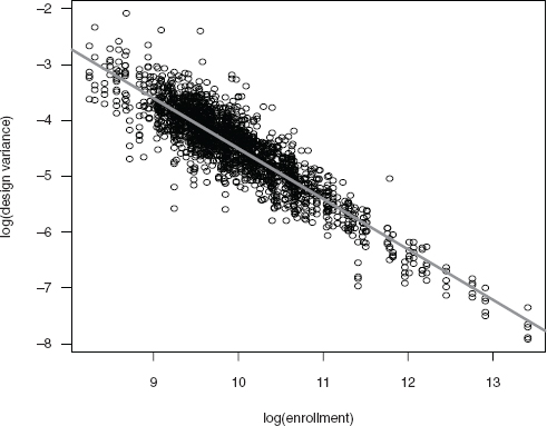
The design variance within a district is determined largely by sample size, which is, in turn, highly correlated with enrollment. Figure F-1 displays a scatter plot of data and the regression model fit for log(design variance) as a function of log(enrollment) for the 1-year ACS estimates in large districts. The fitted linear relationship is given by log(design variance) = 4.5 - 0.9 log(enrollment).
We choose log(enrollment) = 9.8 as a typical value for a large district because it is close to log(median(enrollment)) = 9.84. If we plug this value into the linear relationship above and transform to the design standard deviation, we get 0.1153, which is very close to the average design standard deviation across districts and years, 0.1146. Next, we take the SAS fit, which models gdt = bdt + edt as AR(1), and approximate the fitted AR(1) by AR(1) + uncorrelated noise, where the noise has variance equal to the “typical value” .0133 = (0.1153)2. The resulting model for bdt ~ AR(1) has process variance 0.01548 and autoregressive parameter 0.3168. Finally, taking the model for bdt as fixed, let the variance for edt depend on enrollment through the above linear relationship. Tables F-10 and F-11, discussed above, were constructed using this analysis, with enrollment taken
to be the observed median enrollment for medium districts and for small districts, respectively.
The standard deviation (SD) and coefficient of variation (CV) (relative to mean (CCD) = $1.65) of 1-year change in 5-year estimates for various enrollments are shown in Table F-12.
There are real differences in the amount of noise under which districts normally operate with traditional application and certification procedures. Small districts combined have a percentage standard deviation (CV) of 10.3 percent for CCD 1-year changes, but those with less than the median enrollment have a CV of 11.6 percent, while those with more than the median enrollment have a CV of 8.7 percent. These are comparable to the ACS5 (modeled) CVs at enrollments of 400-800, according to Table F-12, which is the same as Table 4-8 in Chapter 4. Figure F-2, which is the same as Figure 4-5 in Chapter 4, displays a transformation of the data in Table F-12. For a given district, the point (1/enrollment, CV2) can be plotted on the figure. If the plotted point is above the curve, the district currently experiences more variability in its administrative estimates
TABLE F-12 Intertemporal Variability of ACS 5-Year Estimates, by Enrollment
| Variability of 1-Year Change in ACS 5-Year Estimates of Blended Reimbursement Rates |
||
| Enrollment | Standard Deviation ($) | Coefficient of Variation (%) (relative to BRR of $1.65) |
| 100 | 0.34 | 20.5 |
| 200 | 0.25 | 15.1 |
| 400 | 0.18 | 11.2 |
| 800 | 0.14 | 8.3 |
| 1,600 | 0.10 | 6.3 |
| 3,200 | 0.08 | 4.8 |
| 6,400 | 0.06 | 3.8 |
| 12,800 | 0.05 | 3.2 |
SOURCE: Prepared by the panel.
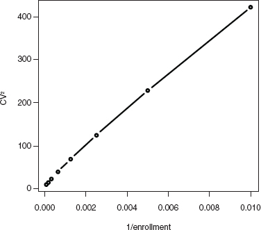
FIGURE F-2 Squared coefficient of variation of year-to-year change in ACS 5-year estimate of BRR versus inverse of enrollment.
NOTES: ACS = American Community Survey; BRR = blended reimbursement rate; CV = coefficient of variation.
SOURCE: Prepared by the panel.
than it would if it used ACS 5-year estimates (at least according to the model and ignoring timeliness bias). In this situation, the district might find use of the ACS 5-year estimates to be acceptable. On the other hand, if its plotted point is below the curve, the district currently experiences less variability in its administrative estimates than it would with the ACS 5-year estimates, and might find the latter unacceptably variable for use in determining reimbursements under the ACS Eligibility Option (AEO).
Table F-13 shows standard deviations, biases, and root mean squared errors (RMSEs) for ACS 1-year, 3-year, and 5-year estimators, with and without a 2-year lag (reflecting the lag in the availability of ACS estimates for use in establishing claiming rates). For large districts, these values are computed in two ways: (1) using the AR(1) model originally fitted via SAS for gdt and (2) using the AR(1) + noise model for gdt. The latter model makes results consistent with the analysis for medium and small districts, all of which use the AR(1) + noise model. The other difference in the AR(1) analysis for the large districts is that bt is estimated from the data (see Box F-7) and incorporated in the bias computations, while in the AR(1) + noise analysis, it is assumed to be constant over time (or zero, without loss of generality). Again this is done to maintain consistency with the analysis for medium and small districts, for which estimation of bt from the data is not possible.
| District Size | ACS1, no lag | ACS1, lag 2 | ACS3, no lag | ACS3, lag 2 | ACS5, no lag | ACS5, lag 2 | |||
| Large | SD (2) | 0.170 | 0.221 | 0.135 | 0.137 | 0.124 | 0.126 | ||
| SD (1) | 0.169 | 0.221 | 0.134 | 0.137 | 0.123 | 0.125 | |||
| Bias (2) | 0.000 | –0.128 | –0.069 | –0.153 | –0.107 | NA | |||
| Bias (1) | –0.025 | –0.143 | –0.096 | –0.131 | –0.107 | ||||
| RMSE (2) | 0.170 | 0.256 | 0.152 | 0.205 | 0.164 | NA | |||
| RMSE (1) | 0.172 | 0.263 | 0.165 | 0.189 | 0.163 | ||||
| Medium | SD | 0.243 | 0.282 | 0.168 | 0.170 | 0.147 | 0.148 | ||
| Bias | 0.000 | –0.115 | –0.062 | –0.130 | –0.092 | NA | |||
| RMSE | 0.243 | 0.304 | 0.179 | 0.214 | 0.173 | NA | |||
| Small | SD | 0.537 | 0.556 | 0.324 | 0.325 | 0.260 | 0.261 | ||
| Bias | 0.000 | –0.104 | –0.059 | –0.107 | –0.079 | NA | |||
| RMSE | 0.537 | 0.565 | 0.329 | 0.342 | 0.271 | NA | |||
NOTES: The results for large districts were obtained using two methods: (1) using the AR(1) model for gdt and (2) using the AR(1) plus noise model for gdt. ACS = American Community Survey; NA = not applicable; RMSE = root mean squared error; SD = standard deviation.
SOURCE: Prepared by the panel.
The bias and RMSE results reflect the specific mt estimated for the particular 5-year time window covered by the estimates available to the panel, separately for each district size class. For any size class, the estimate of mt is simply the year t average CCD BRR across all districts. For large districts, these estimated mt values are given in Box F-7.
This part of the appendix describes the results of the panel’s modeling of the differences between ACS estimates and CCD estimates for the BRR. The analysis was limited to very high FRPL districts with both 5-year ACS estimates and CCD estimates for 2009-2010 in the panel’s evaluation data set prog09.merged.fns. To eliminate outliers that could adversely impact regression results, we excluded any districts that had either a percentage certified for free meals of less than 10 percent or a percentage certified for free or reduced-price meals of less than 20 percent. Districts with missing data for potential predictor variables were also excluded.
The ACS estimate used in the analysis is the 5-year ACS estimate for the BRR (denoted ACS5 BRR below). The CCD estimate used is the BRR based on certification data in the 2009-2010 CCD (denoted CCD0910 BRR below). The dependent variable used in the analysis is the difference between ACS5 BRR and CCD0910 BRR divided by the standard error of ACS5 BRR. This variable is regressed on a variety of predictor variables from the 2009-2010 CCD as described below. Table F-14 provides regression results for a variety of alternative models.
In the table, p is the number of covariates in a model, and FOI stands for “first-order interactions.” The “Additive” model is the most basic model, with no interactions or quadratic terms, and the “FOI, No Factor Interaction” model includes interactions among continuous covariates but not with or among the categorical covariates. Box F-8 lists the covariates used in the modeling. The results of our exploratory analyses of whether a global predictive model could be used for adjusting for differences between ACS and administrative estimates are discussed in Chapter 4.
| Without FRPL Covariates (1,433 districts) | With FRPL Covariates (1,366 districts) | |||||||||||
| Model Covariates | p | R2 | Adj. R2 | RMSE | AIC | p | R2 | Adj. R2 | RMSE | AIC | ||
| Additive | 73 | 0.420 | 0.389 | 1.068 | -6009 | 81 | 0.628 | 0.604 | 0.806 | -6408 | ||
| FOI, No Factor | 159 | 0.572 | 0.519 | 0.917 | -6273 | 258 | 0.779 | 0.727 | 0.621 | -6765 | ||
| Interactions | ||||||||||||
| FOI, No State/Locale | 172 | 0.579 | 0.522 | 0.910 | -6271 | 334 | 0.804 | 0.740 | 0.585 | -6777 | ||
| Interactions | ||||||||||||
| FOI, No State | 317 | 0.650 | 0.550 | 0.830 | -6245 | 542 | 0.855 | 0.760 | 0.503 | -6774 | ||
| Interaction | ||||||||||||
| FOI, All Variables | 717 | 0.782 | 0.563 | 0.655 | -6124 | 981 | 0.923 | 0.728 | 0.366 | -6768 | ||
| FOI and Quadratic | 726 | 0.784 | 0.561 | 0.652 | -6116 | 996 | 0.926 | 0.726 | 0.359 | -6784 | ||
NOTES: The basic model is ![]() ~ covariates. AIC = Akaike Information Criterion; ACS = American Community Survey; FOI = first-order interactions; NA = not applicable; RMSE = root mean squared error.
~ covariates. AIC = Akaike Information Criterion; ACS = American Community Survey; FOI = first-order interactions; NA = not applicable; RMSE = root mean squared error.
SOURCE: Prepared by the panel.
BOX F-8
Covariates Used in Regression Analysis
The covariates in the “Without FRPL” models are as follows:
1. C0910_Num_Enroll (number of enrolled students)
2. C0910_Pct_in Non Reg Sch (percentage of students in nonregular—special education, vocational education, or alternative—schools)
3. C0910_Pct_inChartSch (percentage of students in charter schools)
4. C0910_Pct_inChartNonRegSch (percentage of students in charter or non-regular schools)
5. C0910_Pct_inChartMagSch (percentage of students in charter or magnet schools)
6. C0910_Pct_inChartMagNonRegSch (percentage of students in charter, magnet, or nonregular schools)
7. C0910_Pct_AIAN (percentage of students who are American Indian or Alaska Native)
8. C0910_Pct_AsianHNPI (percentage of students who are Asian, Hawaiian Native, or Pacific Islander)
9. C0910_Pct_Hispanic (percentage of students who are Hispanic)
10. C0910_Pct_Black (percentage of students who are black)
11. C0910_Pct_White (percentage of students who are white)
12. C0910_ChartDistance (index measuring distance to nearby charter-only districts)
13. C0910_ChartDistance_Enroll (index measuring distance to nearby charter-only districts, weighted by charter enrollment)
14. C0910_ChartDistance_Enroll_Rel (index measuring distance to nearby charter-only districts, weighted by charter enrollment relative to district’s enrollment)
15. C_State (state)
16. C_Locale_Type (type of locale as defined in CCD)
The “With FRPL” models add the following covariates:
17. C0910_Pct_Free (percentage of students certified for free meals)
18. C0910_Pct_Reduced (percentage of students certified for reduced-price meals)
19. C0910_Num_Free (number of students certified for free meals)
20. C0910_Num_Reduced (number of students certified for reduced-price meals)
21. C0910_ChartDistance_FRPL (index measuring distance to nearby charter-only districts, weighted by number of charter students certified for free or reduced-price meals)
22. C0910_ChartDistance_FRPL_Rel (index measuring distance to nearby charter-only districts, weighted by number of charter students certified for free or reduced-price meals relative to number in district)
23. C0910_Need (categorical variable for whether percentage of students certified for free or reduced-price meals is < 50, 50-74, or ≥ 75)
24. C0910_CCDSchools_CharterCode (categorical variable for whether all, some, or none of the schools in district are charter schools)
SOURCE: Prepared by the panel.


