
Somewhat analogous to the topics we have covered in previous chapters for hardware systems, this chapter covers software reliability growth modeling, software design for reliability, and software growth monitoring and testing.
Software reliability, like hardware reliability, is defined as the probability that the software system will work without failure under specified conditions and for a specified period of time (Musa, 1998). But software reliability differs in important respects from hardware reliability. Software reliability problems are deterministic in the sense that each time a specific set of inputs is applied to the software system, the result will be the same. This is clearly different from hardware systems, for which the precise moment of failure, and the precise cause of failure, can differ from replication to replication. In addition, software systems are not subject to wear-out, fatigue, or other forms of degradation.
In some situations, reliability errors are attributed to a full system and no distinction is made between subsystems or components, and this attribution is appropriate in many applications. However, as is the case for any failure mode, there are times when it is appropriate to use separate metrics and separate assessments of subsystem or component reliabilities (with respect to system structure as well as differentiating between software and hardware reliability), which can then be aggregated for a full-system assessment. This separate treatment is particularly relevant to software failures given the different nature of software and hardware reliability.
Chapter 4 on hardware reliability growth is primarily relevant to growth that occurs during full-system testing, which is relevant to the
middle and later stages of developmental testing. In contrast, except for when the entire system is software, it is appropriate for software reliability growth to be primarily considered as a component-level concern, which would be addressed while the system is in development by the contractor, or at the latest, during the earliest stages of developmental testing. Therefore, the primary party responsible for software reliability is the contractor.
In this chapter we first discuss software reliability growth modeling as it has been generally understood and used in defense acquisition. We then turn to a new approach, metrics-based modeling: we describe the work that has been done and discuss how to build metrics-based prediction models. The last two sections of the chapter briefly consider testing and monitoring.
SOFTWARE RELIABILITY GROWTH MODELING
Classic Design Models
Software reliability growth models have, at best, limited use for making predictions as to the future reliability of a software system in development for several reasons. Most important, the pattern of reliability growth evident during the development of software systems is often not monotonic because corrections to address defects will at times introduce additional defects. Therefore, although the nonhomogeneous Poisson process model is one of the leading approaches to modeling the reliability of software (and hardware) systems in development, it often provides poor inferences and decision rules for the management of software systems in development.
Other deficiencies in such models relevant to software are the substantial dependence on time as a modeling factor, the dynamic behavior of software systems, the failure to take into consideration various environmental factors that affect software reliability when fielded, and hardware interactions. With respect to the dependence on time, it is difficult to create a time-based reliability model for software systems because it is highly likely that the same software system will have different reliability values in relation to different software operational use profiles. The dynamic behavior of software systems as a function of the environment of use, the missions employed, and the interactions with hardware components, all complicate modeling software reliability.
Siegel (2011, 2012) describes related complexities. Often metric-based models for software reliability, derived from a large body of recent research ranging from code churn, code complexity, code dependencies, testing coverage, bug information, usage telemetry, etc., have been shown to be effective predictors of code quality. Therefore, this discussion of software reliability growth models is followed by a discussion of the use of metric-
based models, which we believe have important advantages as tools for predicting software reliability of a system.
A number of models of software reliability growth are available and represent a substantial proportion of the research on software reliability. They range from the simple Nelson model (Nelson, 1978), to more sophisticated hyper-geometric coverage-based models (e.g., Jacoby and Masuzawa, 1992), to component-based models and object-oriented models (e.g., Basili et al., 1996). Several reliability models use Markov chain techniques (e.g., Whittaker, 1992). Other models are based on the use of an operational profile, that is, a set of software operations and their probabilities of occurrence (e.g., Musa, 1998). These operational profiles are used to identify potentially critical operational areas in the software to signal a need to increase the testing effort in those areas. Finally, a large group of software reliability growth models are described by nonhomogenous Poisson processes (for a description, see Yamada and Osaki, 1985): this group includes Musa (e.g., Musa et al., 1987) and the Goel-Okumoto models (e.g., Goel and Okumoto, 1979).
Software reliability models can be classified broadly into seven categories (Xie, 1991):
- Markov models: A model belongs to this class if its probabilistic assumption of the failure process is essentially a Markov process. In these models, each state of the software has a transition probability associated with it that governs the operational criteria of the software.
- Nonhomogeneous Poisson process models: A model is in this class if the main assumption is that the failure process is described by a nonhomogeneous Poisson process. The main characteristic of this type of model is that there is a mean value function that is defined by the expected number of failures up to a given time.
- Bayesian process models: In a Bayesian process model, some information about the software to be studied is available before the testing starts, such as the inherent fault density and defect information of previous releases. This information is then used in combination with the collected test data to more accurately estimate and make predictions about reliability.
- Statistical data analysis methods: Various statistical models and methods are applied to software failure data. These models include time-series models, proportional hazards models, and regression models.
- Input-domain based models: These models do not make any dynamic assumption about the failure processes. All possible input and output domains of the software are constructed and, on the
- basis of the results of the testing, the faults in mapping between the input and output domains are identified. In other words, for a particular value in the input domain, either the corresponding value in the output domain is produced or a fault is identified.
- Seeding and tagging models: These models are the same as capture-recapture methods based on data resulting from the artificial seeding of faults in a software system. The assessment of a test is a function of the percentage of seeded faults that remain undiscovered at the conclusion of the testing effort.
- Software metrics models: Software reliability metrics, which are measures of the software complexity, are used in models to estimate the number of software faults remaining in the software.
A fair number of these classical reliability models use data on test failures to produce estimates of system (or subsystem) reliability. But for many software systems, developers strive for the systems to pass all the automated tests that are written, and there are often no measurable faults. Even if there are failures, these failures might not be an accurate reflection of the reliability of the software if the testing effort was not comprehensive. Instead, “no failure” estimation models, as described by Ehrenberger (1985) and Miller et al. (1992), may be more appropriate for use with such methodologies.
Another factor that affects classical software reliability models is that in software systems, the actual measurable product quality (e.g., failure rate) that is derived from the behavior of the system usually cannot be measured until too late in the life cycle to effect an affordable corrective action. When test failures occur in actual operation, the system has already been implemented. In general, a multiphase approach needs to be taken to collect the various metrics of the relevant subsystems at different stages of development, because different metrics will be estimable at different development phases and some can be used as early indicators of software quality (for a description of these approaches, see Vouk and Tai, 1993; Jones and Vouk, 1996). In Box 9-1, we provide short descriptions of the classical reliability growth models and some limitations of each approach.
Performance Metrics and Prediction Models
An alternative approach to reliability growth modeling for determining whether a software design is likely to lead to a reliable software system is to rely on performance metrics. Such metrics can be used in tracking software development and as input into decision rules on actions such as accepting subsystems or systems for delivery. In addition to such metrics, there has been recent work on prediction models, some of this stemming from the
BOX 9-1
Overview of Classical Software Reliability Growth Models
Nelson Model
This is a very simplistic model based on the number of test failures:
![]()
where
- R is the system reliability
 is the number of failures during testing
- n is the total number of testing runs.
A limitation of this model is that if no failures are available, the reliability becomes 100 percent, which might not always be the case. For details, see Nelson (1978).
Fault Seeding Models
In these models, faults are intentionally injected into the software by the developer. The testing effort is evaluated on the basis of how many of these injected defects are found during testing. Using the number of injected defects remaining, an estimate of the reliability based on the quality of the testing effort is computed using capture-recapture methods. A limitation of this model is that for most large systems, not all parts have the same reliability profile. The fault seeding could also be biased, causing problems in estimation. For details, see Schick and Wolvertone (1978) and Duran and Wiorkowski (1981).
Hypergeometric Distribution
This approach models overall system reliability by assuming that the number of faults experienced in each of several categories of test instance follows the hypergeometric distribution. However, if all the test cases pass, then there are no faults or failures to analyze. For details, see Tahoma et al. (1989).
Fault Spreading Model
In this model, the number of faults at each level (or testing cycle or stage) is used to make predictions about untested areas of the software. One limitation of the model is the need for data to be available early enough in the development cycle to affordably guide corrective action. For details, see Wohlin and Korner (1990).
Fault Complexity Model
This model ranks faults according to their complexity. The reliability of the system is estimated on the basis of the number of faults in each complexity level (high, moderate, low) of the software. For details, see Nakagawa and Hanata (1989).
Littlewood-Verall Model
In this model, waiting times between failures are assumed to be exponentially distributed with a parameter assumed to have a prior gamma distribution. For details, see Littlewood and Verall (1971).
Jelinski-Moranda (JM) Model
In the JM model, the initial number of software faults is unknown but fixed, and the times between the discovery of failures are exponentially distributed. Based on this set-up, the JM model is modeled as a Markov process model. For details, see Jelinksi and Moranda (1972).
Bayesian Model for Fault Free Probability
This model deals with the reliability of fault-free software. Reliability at time t is assumed to have the following form:
R(t | λ,p) = (1 – p) + pe–λt,
where λ is given by a prior gamma distribution and p (the probability that the software is not fault free) is given by a Beta distribution. Using these two parameters, a Bayesian model is constructed to estimate the reliability. For details, see Thompson and Chelson (1980).
Bayesian Model Using a Geometric Distribution
In this model, based on the number of test cases at the ith debugging instance for which a failure first occurs, the number of failures remaining at the current debugging instance is determined. For details, see Liu (1987).
Goel-Okumoto Model
This is a nonhomogeneous Poisson process model in which the mean of the distribution of the cumulative number of failures at time t is given by m(t) = a(1 – e–bt), where a and b are parameters estimated from the collected failure data. For details, see Goel and Okumoto (1979).
S-Shaped Model
This is also a nonhomogeneous Poisson process model in which the mean of the distribution of the cumulative number of failures is given by m(t) = a(1 –(1 + bt)e–bt)), where a is the expected number of faults detected, and b is the failure detection rate. For details, see Yamada and Osaki (1983).
Basic Execution Time Model
In this model, the failure rate function at time t is given by:
λ(t) = fK(N0 – µ(t)),
where
- f and K are parameters related to the testing phase
- N0 is the assumed initial number of faults, and
- μ(t) is the number of faults corrected after t amount of testing.
A limitation of this model is that it cannot be applied when one does not have the initial number of faults and the failure rate function at execution time t. For details, see Musa (1975).
Logarithmic Poisson Model
This model is related to the basic execution time model (above). However, here the failure rate function is given by:
λ(t) = λ0e–øµ(t)
where λ0 is the initial failure intensity, and ø is the failure intensity decay parameter. For details, see Musa and Okumoto (1984).
Duane Model (Weibull Process Model)
This is a nonhomogeneous Poisson process model with mean function
![]()
The two parameters, α and β, are estimated using failure time data. For details, see Duane (1964).
Markov Models
Markov models require transition probabilities from state to state where the states are defined by the current values of key variables that define the functioning of the software system. Using these transition probabilities, a stochastic model is created and analyzed for stability. A primary limitation is that there can be a very large number of states in a large software program. For details, see Whittaker (1992).
Fourier Series Model
In this model, fault clustering is estimated using time-series analysis. For details, see Crow and Singpurwalla (1984).
Input Domain-Based Models
In these models, if there is a fault in the mapping of the space of inputs to the space of intended outputs, then that mapping is identified as a potential fault to be rectified. These models are often infeasible because of the very large number of possibilities in a large software system. For details, see Bastani and Ramamoorthy (1986) and Weiss and Weyuker (1988).
work of McCabe (1976) and more recent work along similar lines (e.g., Ostrand et al., 2005; Weyuker et al., 2008).
It is quite likely that for broad categories of software systems, there already exist prediction models that could be used earlier in development than performance metrics for use in tracking and assessment. It is possible that such models could also be used to help identify better performing contractors at the proposal stage. Further, there has been a substantial amount of research in the software engineering community on building generalizable prediction models (i.e., models trained in one system to be applied to another system); an example of this approach is given in Nagappan et al. (2006). Given the benefits from earlier identification of problematic software, we strongly encourage the U.S. Department of Defense (DoD) to stay current with the state of the art in software reliability as is practiced in the commercial software industry, with increased emphasis on data analytics and analysis. When it is clear that there are prediction models that are broadly applicable, DoD should consider mandating their use by contractors in software development.
A number of metrics have been found to be related to software system reliability and therefore are candidates for monitoring to assess progress toward meeting reliability requirements. These include code churn, code complexity, and code dependencies (see below).
We note that the course on reliability and maintainability offered by the Defense Acquisition University lists 10 factors for increasing software reliability and maintainability:
- good statement of requirements,
- use of modular design,
- use of higher-order languages,
- use of reusable software,
- use of a single language,
- use of fault tolerance techniques,
- use of failure mode and effects analysis,
- review and verification through the work of an independent team,
- functional test-debugging of the software, and
- good documentation.
These factors are all straightforward to measure, and they can be supplied by the contractor throughout development.
Metrics-based models are a special type of software reliability growth model that have not been widely used in defense acquisition. These are
software reliability growth models that are based on assessments of the change in software metrics that are considered to be strongly related to system reliability. The purpose of this section is to provide an understanding of when metrics-based models are applicable during software development. The standard from the International Organization for Standards and the International Electrotechnical Commission 1498-1 states that “internal metrics are of little value unless there is evidence that they are related to some externally visible quality.” Internal metrics have been shown to be useful, however, as early indicators of externally visible product quality when they are related (in a statistically significant and stable way) to the field quality (reliability) of the product (see Basili et al., 1996).
The validation of such internal metrics requires a convincing demonstration that the metric measures what it purports to measure and that the metric is associated with an important external metric, such as field reliability, maintainability, or fault-proneness (for details, see El-Emam, 2000). Software fault-proneness is defined as the probability of the presence of faults in the software. Failure-proneness is the probability that a particular software element will fail in operation. The higher the failure-proneness of the software, logically, the lower the reliability and the quality of the software produced, and vice versa.
Using operational profiling information, it is possible to relate generic failure-proneness and fault-proneness of a product. Research on fault-proneness has focused on two areas: the definition of metrics to capture software complexity and testing thoroughness and the identification of and experimentation with models that relate software metrics to fault-proneness (see, e.g., Denaro et al., 2002). While software fault-proneness can be measured before deployment (such as the count of faults per structural unit, e.g., lines of code), failure-proneness cannot be directly measured on software before deployment.
Five types of metrics have been used to study software quality: (1) code churn measures, (2) code complexity measures, (3) code dependencies, (4) defect or bug data, and (5) people or organizational measures. The rest of this section, although not comprehensive, discusses the type of statistical models that can be built using these measures.
Code Churn
Code churn measures the changes made to a component, file, or system over some period of time. The most commonly used code churn measures are the number of lines of code that are added, modified, or deleted. Other churn measures include temporal churn (churn relative to the time of release of the system) and repetitive churn (frequency of changes to the same file or component). Several research studies have used code churn as an indicator
of code quality (fault- or failure-proneness and, by extension, reliability). Graves et al. (2000) predicted fault incidences using software change history on the basis of a time-damping model that used the sum of contributions from all changes to a module, in which large or recent changes contributed the most to fault potential. Munson and Elbaum (1998) observed that as a system is developed, the relative complexity of each program module that has been altered will change. They studied a software component with 300,000 lines of code embedded in a real-time system with 3,700 modules programmed in C. Code churn metrics were found to be among the most highly correlated with problem reports.
Another kind of code churn is debug churn, which Khoshgoftaar et al. (1996) define as the number of lines of code added or changed for bug fixes. The researchers’ objective was to identify modules in which the debug code churn exceeded a threshold in order to classify the modules as fault-prone. They studied two consecutive releases of a large legacy system for telecommunications that contained more than 38,000 procedures in 171 modules. Discriminant analysis identified fault-prone modules on the basis of 16 static software product metrics. Their model, when used on the second release, showed type I and type II misclassification rates of 21.7 percent and 19.1 percent, respectively, and an overall misclassification rate of 21.0 percent.
Using information on files with status new, changed, and unchanged, along with other explanatory variables (such as lines of code, age, prior faults) as predictors in a negative binomial regression equation, Ostrand et al. (2004) successfully predicted the number of faults in a multiple release software system. Their model had high accuracy for faults found in both early and later stages of development.
In a study on Windows Server 2003, Nagappan and Ball (2005) demonstrated the use of relative code churn measures (normalized values of the various measures obtained during the evolution of the system) to predict defect density at statistically significant levels. Zimmermann et al. (2005) mined source code repositories of eight large-scale open source systems (IBM Eclipse, Postgres, KOffice, gcc, Gimp, JBoss, JEdit, and Python) to predict where future changes would take place in these systems. The top three recommendations made by their system identified a correct location for future change with an accuracy of 70 percent.
Code Complexity
Code complexity measures range from the classical cyclomatic complexity measures (see McCabe, 1976) to the more recent object-oriented metrics, one of which is known as the CK metric suite after its authors (see Chidamber and Kemerer, 1994). McCabe designed cyclomatic complexity
as a measure of the program’s testability and understandability. Cyclomatic complexity is adapted from the classical graph theoretical cyclomatic number and can be defined as the number of linearly independent paths through a program. The CK metric suite identifies six object-oriented metrics:
- weighted methods per class, which is the weighted sum of all the methods defined in a class;
- coupling between objects, which is the number of other classes with which a class is coupled;
- depth of inheritance tree, which is the length of the longest inheritance path in a given class;
- number of children, which is the count of the number of children (classes) that each class has;
- response for a class, which is the count of the number of methods that are invoked in response to the initiation of an object of a particular class; and
- lack of cohesion of methods, which is a count of the number of method pairs whose similarity is zero minus the count of method pairs whose similarity is not zero.
The CK metrics have also been investigated in the context of fault-proneness. Basili et al. (1996) studied the fault-proneness in software programs using eight student projects. They found the first five object-oriented metrics listed above were correlated with defects while the last metric was not. Briand et al. (1999) obtained somewhat related results. Subramanyam and Krishnan (2003) present a survey on eight more empirical studies, all showing that object-oriented metrics are significantly associated with defects. Gyimóthy et al. (2005) analyzed the CK metrics for the Mozilla codebase and found coupling between objects to be the best measure in predicting the fault-proneness of classes, while the number of children was not effective for fault-proneness prediction.
Code Dependencies
Early work by Pogdurski and Clarke (1990) presented a formal model of program dependencies based on the relationship between two pieces of code inferred from the program text. Schröter et al. (2006) showed that such dependencies can predict defects. They proposed an alternate way of predicting failures for Java classes. Rather than looking at the complexity of a class, they looked exclusively at the components that a class uses. For Eclipse, the open source integrated development environment, they found that using compiler packages resulted in a significantly higher failure-proneness (71 percent) than using graphical user interface packages
(14 percent). Zimmermann and Nagappan (2008) built a systemwide code dependency graph of Windows Server 2003 and found that models built from (social) network measures had accuracy of greater than 10 percentage points in comparison with models built from complexity metrics.
Defect Information
Defect growth curves (i.e., the rate at which defects are opened) can also be used as early indicators of software quality. Chillarege et al. (1991) at IBM showed that defect types could be used to understand net reliability growth in the system. And Biyani and Santhanam (1998) showed that for four industrial systems at IBM there was a very strong relationship between development defects per module and field defects per module. This approach allows the building of prediction models based on development defects to identify field defects.
People and Social Network Measures
Meneely et al. (2008) built a social network between developers using churn information for a system with 3 million lines of code at Nortel Networks. They found that the models built using such social measures revealed 58 percent of the failures in 20 percent of the files in the system. Studies performed by Nagappan et al. (2008) using Microsoft’s organizational structure found that organizational metrics were the best predictors for failures in Windows.
BUILDING METRICS-BASED PREDICTION MODELS
In predicting software reliability with software metrics, a number of approaches have been proposed. Logistic regression is a popular technique that has been used for building metric-based reliability models. The general form of a logistic regression equation is given as follows:
![]()
where c, a1, and a2 are the logistic regression parameters and X1, X2, … are the independent variables used for building the logistic regression model. In the case of metrics-based reliability models, the independent variables can be any of the (combination of) measures ranging from code churn and code complexity to people and social network measures.
Another common technique used in metrics-based prediction models is a support vector machine (for details, see Han and Kamber, 2006). For a quick overview of this technique, consider a two-dimensional training set with two classes as shown in Figure 9-1. In part (a) of the figure, points representing software modules are either defect-free (circles) or have defects (boxes). A support vector machine separates the data cloud into two sets by searching for a maximum marginal hyperplane; in the two-dimensional case, this hyperplane is simply a line. There are an infinite number of possible hyperplanes in part (a) of the figure that separate the two groups. Support vector machines choose the hyperplane with the margin that gives the largest separation between classes. Part (a) of the figure shows a hyperplane with a small margin; part (b) shows one with the maximum margin. The maximum margin is defined by points from the training data—these “essential” points are also called support vectors; in part (b) of the figure they are indicated in bold.
Support vector machines thus compute a decision boundary, which is used to classify or predict new points. One example is the triangle in part (c) of Figure 9-1. The boundary shows on which side of the hyperplane the new software module is located. In the example, the triangle is below the hyperplane; thus it is classified as defect free.
Separating data with a single hyperplane is not always possible. Part (d) of Figure 9-1 shows an example of nonlinear data for which it is not possible to separate the two-dimensional data with a line. In this case, support vector machines transform the input data into a higher dimensional space using a nonlinear mapping. In this new space, the data are then linearly separated (for details, see Han and Kamber, 2006). Support vector machines are less prone to overfitting than some other approaches because the complexity is characterized by the number of support vectors and not by the dimensionality of the input.
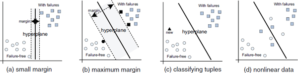
FIGURE 9-1 Support vector machines: overview.
NOTE: See text for discussion.
Other techniques that have been used instead of logistic regression and support vector machines are discriminant analysis and decision and classification trees.
Drawing general conclusions from empirical studies in software engineering is difficult because any process is highly dependent on a potentially large number of relevant contextual variables. Consequently, the panel does not assume a priori that the results of any study will generalize beyond the specific environment in which it was conducted, although researchers understandably become more confident in a theory when similar findings emerge in different contexts.
Given that software is a vitally important aspect of reliability and that predicting software reliability early in development is a severe challenge, we suggest that DoD make a substantial effort to stay current with efforts employed in industry to produce useful predictions.
There is a generally accepted view that it is appropriate to combine software failures with hardware failures to assess system performance in a given test. However, in this section we are focusing on earlier non-system-level testing in developmental testing, akin to component-level testing for hardware. The concern is that if insufficient software testing is carried out during the early stages of developmental testing, then addressing software problems discovered in later stages of developmental testing or in operational testing will be much more expensive.1
As discussed in National Research Council (2006), to adequately test software, given the combinatorial complexity of the sequence of statements activated as a function of possible inputs, one is obligated to use some form of automated test generation, with high code coverage assessed using one of the various coverage metrics proposed in the research literature. This is necessary both to discover software defects and to evaluate the reliability of the software component or subsystem. However, given the current lack of software engineering expertise accessible in government developmental testing, the testing that can be usefully carried out, in addition to the testing done for the full system, is limited. Consequently, we recommend that the primary testing of software components and subsystems be carried out by the developers and carefully documented and reported to DoD and that contractors provide software that can be used to run automated tests of the component or subsystem (Recommendation 14, in Chapter 10).
_______________
1 By software system, we mean any system that is exclusively software. This includes information technology systems and major automated information systems.
If DoD acquires the ability to carry out automated testing, then there are model-based techniques, including those developed by Poore (see, e.g., Whittaker and Poore, 1993), based on profiles of user inputs, that can provide useful summary statistics about the reliability of software and its readiness for operational test (for details, see National Research Council, 2006).
Finally, if contractor code is also shared with DoD, then DoD could validate some contractor results through the use of fault injection (seeding) techniques (see Box 9-1, above). However, operational testing of a software system can raise an issue known as fault masking, whereby the occurrence of a fault prevents the software system from continuing and therefore misses faults that are conditional on the previous code functioning properly. Therefore, fault seeding can fail to provide unbiased estimates in such cases. The use of fault seeding could also be biased in other ways, causing problems in estimation, but there are various generalizations and extensions of the technique that can address these various problems. They include explicit recognition of order constraints and fault masking, Bayesian constructs that provide profiles for each subroutine, and segmenting system runs.
One of the most important principles found in commercial best practices is the benefit from the display of collected data in terms of trend charts to track progress. Along these lines, Selby (2009) demonstrates the use of analytics dashboards in large-scale software systems. Analytics dashboards provide easily interpretable information that can help many users, including front-line software developers, software managers, and project managers. These dashboards can cater to a variety of requirements: see Figure 9-2. Several of the metrics shown in the figure, for example, the trend of post-delivery defects, can help assess the overall stability of the system.
Selby (2009) states that organizations should define data trends that are reflective of success in meeting software requirements so that, over time, one could develop statistical tests that could effectively discriminate between successful and unsuccessful development programs. Analytics dashboards can also give context-specific help, and the ability to drill down to provide further details is also useful: see Figure 9-3 for an example.
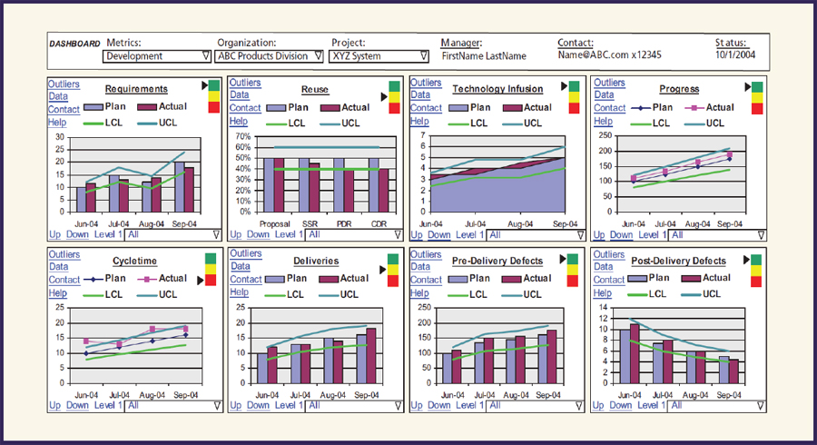
FIGURE 9-2 Analytics dashboards.
SOURCE: Selby (2009, p. 42). Reprinted with permission.
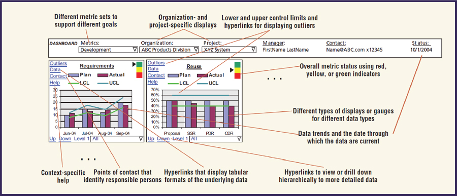
FIGURE 9-3 Example of a specific context of an analytics dashboard.
SOURCE: Selby (2009). Reprinted with permission.


