
5
Policy Responses to an Aging Population
The long-term fiscal imbalance in the Social Security system will ultimately require policy makers to make changes to put the system on firmer financial footing. Many reform proposals have been advanced to improve solvency; most involve some form of tax increase or benefit reduction (at least relative to the level promised in the past), which are fundamentally the only ways to address Social Security’s long-term imbalance. The complexity of the Social Security program, though, means that there are many different options for reform within these categories of adjustments, and they can be combined in multiple ways. A Congressional Budget Office study, for example, evaluated 30 possible reforms (Congressional Budget Office, 2010), and an October 2014 update on the website of the Office of the Chief Social Security Actuary considers the impact of 37 long-range Social Security policy provisions.1Box 5-1 considers the direct indexation of benefit levels to changes in mortality within a population.
SOCIAL SECURITY POLICY SIMULATIONS
The committee’s analysis simulates six possible Social Security reforms. We believe these reforms are particularly relevant because either they are frequently discussed in policy circles or they meet objectives that many stakeholders would agree with, such as that benefit reductions should be crafted so as to avoid harming low-income workers. The choice of reforms to analyze has also been influenced by what is possible given the current
________________
1See http://www.socialsecurity.gov/OACT/solvency/provisions/index.html [March 2015].
BOX 5-1
Indexing Social Security Benefit Levels to Mortality Changes
An alternative to raising the normal retirement age (NRA) in response to increases in longevity is to directly index initial benefits (i.e., the annual benefit received by a worker when initially claiming benefits) instead. For example, Diamond and Orszag (2004) proposed that both initial benefit levels and the payroll tax rate be indexed each year to offset the impact on Social Security’s finances from observed changes in life expectancy. Under their proposal, Social Security’s chief actuary would compute each year the net impact on Social Security’s actuarial imbalance from the change in life expectancy for a typical worker claiming benefits at the NRA. Half of this net impact would then be offset by raising the payroll tax rate, and half by reducing initial benefit levels for cohorts of workers who have not yet reached the early entitlement age. Diamond and Orszag argued that this approach is preferable to raising the NRA itself, because it incorporates both benefit reductions and revenue increases as adjustments to increases in life expectancy and because directly adjusting initial benefit levels avoids many of the anomalies in the pattern of benefit reductions by age associated with raising the NRA.
In theory, this approach could be used to adjust benefit levels at each lifetime earnings quintile and thereby offset not only the change in average life expectancy but also the change in the distribution of life expectancy with respect to lifetime earnings. Furthermore, this approach could be applied for any given mix of revenue and benefit adjustments to the actuarial impact from the change in average life expectancy. In particular, within the benefit component of the annual adjustment, the chief actuary could estimate the change in life expectancy by
structure of the Future Elderly Model (FEM); for example, Although the committee would have liked to simulate the effect of raising the taxable maximum earnings base—a popular proposal on the revenue side—this was not feasible within the existing FEM.
The Social Security reforms simulated for this report include
- raising the Social Security early entitlement age (EEA) by 2 years, to age 64;
- raising the Social Security normal retirement age (NRA) by 3 years, to age 70;
- raising both the EEA as in policy 1 and the NRA as in policy 2;
- reducing the cost-of-living adjustment (COLA) applied to benefits by 0.2 percent per year, starting at age 62;
- reducing the top primary insurance amount (PIA) factor by one-third, from 15 percent to 10 percent (applies to average indexed
quintile of average indexed monthly earnings, based on mortality experience over the previous 12 months for retirees in that quintile of earnings, and also estimate the impact on Social Security’s lifetime benefits from that change. The chief actuary would then apply adjustment factors to the benefit levels across quintiles in order to offset, at least approximately, the impact of the change in life expectancy distribution on the pattern of lifetime benefits. For example, if the top quintile accounted for 50 percent of the increase in the present value of lifetime benefits from the overall changes in mortality, the top quintile’s annual benefit would be reduced such that, on average, those reductions accounted for 50 percent of the overall reduction in annual benefits from the adjustment. The goal of the process would be to keep the distribution of lifetime benefits invariant to changes in the distribution of life expectancy. As noted in Chapter 4 of this report, whether or not that goal is desirable is debatable.
In practice, this approach would have several implementation challenges. First, the mortality experience by earnings quintile in each year will be more variable than the average. To mitigate this variability, the adjustment by quintile could be done less often, perhaps every 5 years rather than every year. Second, the adjustment factors would have to be smoothed to avoid discontinuities just above and below the quintile threshold, and the smoothing process would have to be specified ahead of time. Third, the process would need to reconcile the adjustment factors by quintile and the bend points in the Social Security benefit formula, which is technically challenging. Finally, because the process would introduce some uncertainty around benefit levels for workers nearing retirement, it might be desirable to apply the adjustment factors only to future retirement benefits for workers below a certain age (such as 55 or 60).
-
monthly earnings [AIME] amounts beyond the second bend point, currently $4,917); and
- reducing the top PIA factor from 15 percent to 0 percent (applies to AIME amounts beyond the second bend point) and reducing the second bend point to the median AIME.
Note that, with the exception of simulation 3, the analysis changes just one policy per simulation while holding other policies constant. For example, in simulation 1, the EEA rises by 2 years while all other thresholds (the NRA, the age of eligibility for Medicare benefits, etc.) remain unchanged.
There are two mechanisms by which a policy change may translate into an increase or decrease in Social Security and other benefits relative to the baseline scenario. The first channel, which can be characterized as the “mechanical effect,” results directly from the policy change, holding behavior constant. For example, consider the reform in simulation 2, which
raises the NRA by 3 years. A worker claiming Social Security benefits at age 67 would receive 100 percent of his PIA before the NRA reform and 80 percent of his PIA after the reform, so he experiences a 20 percent benefit reduction if he maintains the same claiming age of 67.
The second channel, which can be characterized as the “behavioral effect,” results from any changes in individual behavior in response to the policy.2 Facing an NRA of 70 rather than 67 changes an individual’s incentives and may lead that individual to claim Social Security later, work longer, or even claim disability insurance (DI) benefits. Such behavioral responses can be captured by the FEM. As described earlier, the committee’s analysis first estimated transition models (over a 2-year period) between benefit-related states including working, Social Security claiming, and DI claiming using data from the Health and Retirement Study (HRS). Then the estimates from these models were used to simulate a particular cohort’s patterns of work, claiming, etc. and that cohort’s resulting Social Security and other benefits under the baseline (no reform) scenario. Finally, the policy change(s) for the specific simulation were imposed and the resulting FEM estimates were used to simulate the cohort’s new patterns of behaviors and benefits.3
Predicting new patterns of retirement behavior and how retirement decisions might change in response to various policy changes is a challenging modeling exercise. The approach the committee adopted for predicting retirement choices is based on what economists call a “reduced-form model.” The annex to this chapter provides a discussion of this approach compared to alternative approaches; it also discusses the sensitivity of the results to the committee’s choice of approach.
The post-reform benefits presented in the figures below for each simula-
________________
2Gruber and Wise (2007) discussed the impact of Social Security reforms in terms of mechanical and behavioral effects, and they conducted simulations that decompose the total effect into these two components.
3To continue with the example of the NRA increase, one of the variables in the Social Security claiming model is the number of months until the claimant reaches the NRA. For a worker at age 67, the value for this variable would be changed from 0 to 36 months as one simulates the policy change of a 3-year increase in NRA. The estimated-months-until-NRA coefficient from the Social Security claiming model would be used to predict this individual’s new probability of claiming Social Security at age 67. If that coefficient suggests that the claiming probability increases as an individual approaches the NRA, then moving that person from 0 to 36 months away from the NRA will reduce his or her estimated probability of claiming this year. Claiming later will raise expected benefits if the actuarial adjustment is more than fair, potentially mitigating some of the benefit cut that occurs via the mechanical channel.
tion reflect the combined effect of mechanical and behavioral effects.4 The discussion below contrasts post-reform benefits to the baseline benefits presented in Chapter 4 (see Box 5-2). The committee’s primary focus is on how these simulations affect the progressivity of Social Security and other programs for the elderly. We define progressivity in terms of the ratio of net benefits to inclusive wealth, which the committee views as a good summary measure of an individual’s ability to pay. In particular, net benefits (i.e., benefits minus taxes after age 50, in present value) are progressive if the ratio of benefits in present value to wealth falls as income increases. Based on this definition, a policy change increases progressivity if the net benefit-wealth ratio falls more, or rises less, for those in higher lifetime earnings quintiles than for those in lower quintiles.
Policy Simulation 1: Raising the EEA to Age 64
An increase in the EEA is a frequently discussed policy reform. The 1983 Social Security amendments that legislated increases over time in the NRA did not change the EEA but did increase the penalty for claiming at the EEA. Beneficiaries claiming at age 62 receive a benefit equal to 70 percent of PIA with an NRA of 67, versus 80 percent of PIA under the old NRA of 65. Discussions of potential further increases in the NRA inevitably raise the question of whether the EEA should also be raised, and, if not, what would happen to the penalty for claiming at the EEA. There has also been a related discussion about whether eligibility for retirement benefits, particularly at a relatively early age, might be based on factors other than age (see Box 5-3).
At first glance, it would seem that raising the EEA should have little effect on Social Security’s finances, given the common belief that the actuarial adjustment for early claiming is roughly actuarially fair.5 An increase in the EEA to age 64 would force individuals who would otherwise claim at ages 62 and 63 to claim at age 64 (or later); these individuals would have a higher monthly benefit but would receive benefits for fewer years, and the two effects would essentially cancel each other out. To be sure, even if the adjustment is actuarially fair for the beneficiary population as a whole, it
________________
4Although it is a common practice to associate changes in benefits with changes in well-being, one should use caution in doing so. In particular, although the mechanical changes in benefits may provide an accurate measure of the changes in individual well-being in the absence of behavioral responses, changes in benefits associated with behavioral responses do not fully account for associated changes in well-being because they do not take into account the impact of changes in leisure and other consumption because of, for example, changes in retirement or benefit take-up decisions.
5As noted in Chapter 4, Shoven and Slavov (2013) argue that the actuarial adjustment for the population as a whole is becoming more than fair (indicating that there are greater expected benefits available by delaying claiming) over time.
BOX 5-2
The Experiment
The committee’s simulation experiment calculates the net present value (NPV) of expected taxes paid and government benefits received by a generation over the rest of its life, starting at age 50. The program rules are assumed to remain as defined in 2010 and to persist through subsequent years until all members of the generation have died. The taxes and benefits by age are projected forward, conditional on these rules and on additional assumptions including income growth and health care cost growth. The NPV depends on the proportion of the generation surviving to each future year because only survivors pay taxes and receive benefits. The actual experiment the committee carried out is described under C below, but as an aid to readers we describe two simpler experiments under A and B, to build up to the conditions simulated in C.
- Calculate the NPV at age 50 under two different mortality assumptions: (1) the mortality regime experienced by the cohort born in 1930 (actual, fitted, and projected) and alternatively, and (2) the mortality projected for the cohort born in 1960. Because the mortality projected for the 1960 generation is lower than for the 1930 cohort, the NPV calculated based on its mortality will be higher because benefits are received for more years and at older ages benefits tend to exceed taxes. In this experiment everything other than mortality is held constant.
- This experiment is identical to A except that it is carried out separately by income quintile for each of the two generations. In this experiment, as in A, everything other than mortality is held constant across the two simulations for each income quintile.
- Because mortality differs between the two experimental scenarios for each income quintile, one can expect that health and disability may differ between them as well. A person who dies younger and therefore receives Social Security benefits for fewer years would likely also receive more health care benefits during those years and would be more likely to have received disability benefits. Ignoring these associated variations in health-related benefits would risk overestimating the differences in NPV under the two mortality regimes. These variations in health and functional status by age and sex across the income quintiles will also alter to some degree the simulated trajectories of labor income, benefits, and tax payments. Therefore, in the experimental simulations actually used for the report, the mortality regime for each gender-quintile-birth cohort is paired with its own initial health status and subsequent health and functional status trajectories. With this approach, differences in NPV arise not only because of differences in survival but also because of differences in benefits arising from the associated differences in health and disability status and to the effects of health and disability on earnings trajectories and tax payments.
BOX 5-3
Should Eligibility for Retirement Benefits Be
Based on Factors Other Than Age?
In some countries, eligibility for retirement benefits can occur through years of work rather than age. In Brazil, for example, in addition to an eligibility criterion based on age, the country provides an alternative based on years worked: men can retire after 35 years of contributions and women after 30 years, regardless of age.
A team of researchers associated with the Center for Retirement Research at Boston College has examined similar proposals, which would link the early entitlement age (EEA) in the United States to years of work (Haverstick et al., 2007). Their results showed a positive correlation between lifetime earnings (or wealth or education) and years of work, so linking eligibility to years of work may disproportionately impede access to benefits for low-income workers relative to high-income ones.
For example, among male workers at age 62 between 1992 and 2004, 80 percent of those in the top quintile of the wealth distribution and 67 percent of college graduates attained 35 or more years of covered earnings under Social Security. Among workers in the bottom quintile of the wealth distribution, the share was only 46 percent, and among workers with less than a high school degree, the share was 60 percent. Tying the EEA to years of work would thus pose greater challenges for low-wealth and less-educated workers than others.
Haverstick and colleagues (2007) instead proposed tying the EEA to the AIME. Specifically, they proposed dividing workers into three groups based on their AIME at age 55. Group 1 would include workers with an AIME no higher than 50 percent of the average monthly earnings for all workers. Group 2 would include those with an AIME between 50 and 100 percent of the average, and Group 3 would include workers with above-average AIME. Under the proposal, the first group’s EEA would remain at 62; the second group’s EEA would increase by about one-half month for each percentage point increase in the AIME as a percentage of average earnings above the 50 percent threshold, and the third group’s EEA would increase to 64.
An innovative component of this proposal is to base the EEA for each worker on the value of the worker’s AIME measured at age 55. As the authors noted, “A primary reason for this approach is to allow individuals time to adjust their retirement plans….over half of men ages 50 to 55 have a financial planning horizon of less than 5 years” (Haverstick et al., 2007, p. 15). So, finalizing an individual’s EEA at age 55 should provide sufficient time for individuals to adjust their retirement planning in response to their applicable EEA. In some cases, being notified of one’s EEA at age 55 might also provide a useful “wake up call” to plan for retirement.
will not be fair for every individual or for identifiable subsegments of the population. The earlier discussion of ex ante and ex post redistribution is relevant here. An individual who ends up dying, say, at age 65 is made worse off when the EEA is raised because he receives the higher benefit for only a short time. But Social Security always involves transfers between the short and long lived, and this type of ex post redistribution is generally not viewed as problematic, as discussed above. However, if there are identifiable groups with different life expectancies, then delayed claiming is a better deal for some groups than others on an ex ante basis. In this case, a policy that forces people to claim later than they otherwise would have will raise expected benefits for groups with longer life expectancies while lowering them for groups with shorter life expectancies.
Figure 5-1 shows the average Social Security benefits by earnings quintile for males in the 1930 and 1960 cohorts under the policy experiment that the EEA has been raised to age 64; results from the baseline scenario with an EEA of 62 are shown for comparison. Benefits for the lowest-income males (quintile 1) in the 1930 cohort rise modestly by $1,000 when the EEA is increased, from $126,000 to $127,000. Thus, the adjustment of Social Security benefits is close to actuarially fair for the lowest-income quintile (the change in benefits is well under 1 percent of expected lifetime benefits), which also has the lowest life expectancy. The increase in expected benefits is just slightly larger in the higher income quintiles that have lon-
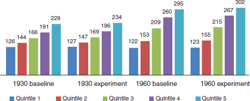
FIGURE 5-1 Average lifetime Social Security benefits for males (in thousands of dollars). Baseline compared with raising the early entitlement age to 64.
SOURCE: Committee generated using Health and Retirement Study data and cohort assumptions.
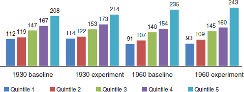
FIGURE 5-2 Average lifetime Social Security benefits for females (in thousands of dollars). Baseline compared with raising the early entitlement age to 64.
SOURCE: Committee generated using Health and Retirement Study data and cohort assumptions.
ger life expectancies ($3,000 for quintile 3 and $5,000 for quintiles 4 and 5) and represents 2 to 3 percent of baseline lifetime benefits. In essence, the delayed claiming that results from an increase in the EEA is slightly more beneficial to these higher-income groups because of their longer life expectancies.
In the 1960 cohort, the effect is similar, with benefits for the lowest-income quintile rising by $1,000 while benefits for the highest-income quintile rising by $7,000. The difference between lowest and highest quintiles (which is larger for the 1960 cohort than for the 1930 cohort for reasons discussed in Chapter 4) is 145 percent of bottom quintile benefits after the EEA increase, versus 142 percent in the baseline scenario.
The results for females, shown in Figure 5-2, are similar. For the 1930 cohort, the policy change raises benefits by $2,000 for the lowest-income quintile and by $6,000 for the highest-income quintile. As a result, the difference between the top and bottom quintiles rises from 86 percent of bottom quintile benefits in the baseline scenario to 88 percent after the EEA increase. For the 1960 cohort, the difference between top and bottom quintiles rises from 158 percent of the bottom quintile value at baseline (as for males, the gap between quintiles 1 and 5 is much larger for the 1960 cohort) to 162 percent after the policy change.
The effect of this policy change on total benefits, shown in Figures 5-3 and 5-4, is essentially the same as the effect on Social Security benefits alone. Total benefits increase by $10,000 or less for all quintiles and cohorts as a result of the policy change, with somewhat larger increases in the higher-income quintiles and for the 1960 cohort.
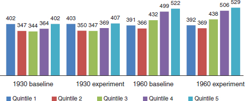
FIGURE 5-3 Average lifetime total benefits for males (in thousands of dollars). Baseline compared with raising the early entitlement age to 64.
SOURCE: Committee generated using Health and Retirement Study data and cohort assumptions.
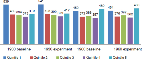
FIGURE 5-4 Average lifetime total benefits for females (in thousands of dollars). Baseline compared with raising the early entitlement age to 64.
SOURCE: Committee generated using Health and Retirement Study data and cohort assumptions.
As noted above, the percentage point change in net benefits as a share of wealth is a useful metric for examining the distributional effect of a policy change. Table 5-1 shows how the policy change would affect lifetime benefits by earnings quintile, based on 1960 mortality rates and relative to the committee’s measure of inclusive wealth. For both males and females, the policy shift would increase benefits as a share of wealth by more for higher earners than for lower earners. For males in the top quintile, for example, the change would increase benefits by 0.4 percent of baseline wealth
TABLE 5-1 Impact of Raising the Early Entitlement Age to 64
| Present value of net benefits at age 50, relative to wealth, based on the mortality profile for those born in 1960 | ||||
| Earnings Quintile | Baseline | Under Policy Experiment | Percentage Point Change | |
| Males | ||||
|
Lowest |
45.6 |
45.7 |
0.1 |
|
|
2 |
36.8 |
37.0 |
0.2 |
|
|
3 |
33.3 |
33.8 |
0.5 |
|
|
4 |
28.9 |
29.3 |
0.5 |
|
|
Highest |
21.4 |
21.7 |
0.4 |
|
| Females | ||||
|
Lowest |
65.4 |
65.6 |
0.2 |
|
|
2 |
54.8 |
55.1 |
0.3 |
|
|
3 |
44.9 |
45.5 |
0.6 |
|
|
4 |
33.5 |
34.1 |
0.6 |
|
|
Highest |
30.8 |
31.4 |
0.6 |
|
SOURCE: Committee generated using Health and Retirement Study data and cohort assumptions.
based on the 1960 mortality projections; for those in the bottom quintile, in contrast, the change would increase benefits by 0.1 percent of baseline wealth. The patterns are broadly similar for females. In all cases, though, the change amounts to less than 1 percent of baseline wealth. The key takeaway point is that an increase in the EEA would make the Social Security system, and thus old-age benefits in general, slightly less progressive.
It is important to recall that the committee’s analysis focuses on the change in net benefits. If a worker chooses to work longer in response to a policy change, then his or her AIME may rise and this will be reflected in a further change to the Social Security benefits. But our analysis does not focus on the additional earnings that might result from a policy change, even though they may raise the worker’s overall well-being.
It is worth noting that this policy change, if enacted on its own, would not generate any savings for the Social Security system, because the projections suggest that benefits would in fact increase slightly. The implication is that individuals tend to claim a little “too early” relative to what would maximize lifetime benefits; on average, therefore, their lifetime benefits would increase if they were forced to delay their claiming. The total cost of benefits would rise by 2 percent for the male population and by 3 percent for the female population. We next discuss the effect of raising the NRA,
a policy that would generate substantial savings, before exploring the scenario where the EEA and NRA are raised simultaneously.
Policy Simulation 2: Increasing the NRA to Age 70
The second simulation analyzed by the committee raises the NRA to age 70. The fact that Social Security’s long-run fiscal imbalance is due in part to rising life expectancy may help to explain why this is a frequently suggested reform. As individuals live longer, the argument goes, it may not be feasible for them to spend all of these additional years of life in retirement; rather, it may be necessary to lengthen one’s work life as well as the period of retirement. Although the NRA is not a “retirement age” in the traditional sense of the word, an increase in the NRA may signal to workers the need to remain in the labor force longer and claim benefits later.
The potential effect on benefits of an NRA increase was explained in the simulation overview above. Absent any change in behavior, the NRA increase functions as a benefit reduction and expected Social Security benefits will fall. Workers may also choose to respond to the policy change by working longer and claiming later; if the actuarial adjustment is more than fair, then doing so will increase benefits, offsetting to some (perhaps small) extent the mechanical effect of the policy change. See Box 5-4 for another view of eligibility ages, one which might allow workers to access benefits before the EEA or to claim benefits before the NRA with a smaller than usual actuarial reduction if they meet certain conditions.
Figures 5-5 and 5-6 show expected Social Security benefits under the simulation’s NRA-increase policy for males and females, respectively. As expected, benefits are noticeably lower than in the baseline scenario. For males in the 1930 cohort, the policy reduces benefits by $31,000, or nearly 25 percent of baseline benefits, for the lowest-income group and by $50,000, or 22 percent of benefits, for the highest-income group.
Because the lowest-income group experiences a proportionately larger decline in benefits, the gap between top and bottom quintiles as a share of bottom quintile benefits grows from 82 percent in the baseline to 88 percent in this simulation. The ratio of top quintile to bottom quintile lifetime benefits similarly rises from 1.82 to 1.88. In other words, although benefits fall for all groups, they decline by a bit more, relative to their initial value, for the lowest-income group.
As the mechanical effect of the cut would be largely the same for all groups in percentage terms,6 the differences in the effect of the policy by income group must result mostly from some combination of two factors.
________________
6Though not precisely the same, because of different proportions of claimers above and below the previous NRA by quintile.
BOX 5-4
Eligibility for Retirement Benefits Based
on Years of Contributions
Several of the policy proposals explored in this chapter involve raising the early entitlement age (EEA), normal retirement age (NRA), or both. Implicit in such proposals is the principle that as longevity increases, workers should expect to spend more years in the labor force and to retire later. Yet workers’ ability to extend their work lives is likely to be heterogeneous. For example, those who have physically demanding jobs may have difficulty working into their mid and late 60s. Similarly, there may be workers who have experienced a late-career job loss and struggled to find new work, particularly in times of economic downturn. Although the disability insurance (DI) program exists to assist those who are too sick to continue working, there may be individuals who do not meet DI eligibility criteria yet would struggle to support themselves while waiting to reach a later EEA or NRA. One possible way to address this concern is to allow workers to access benefits before the EEA or to claim benefits before the NRA with a smaller than usual actuarial reduction if they meet certain conditions. This practice has been adopted by some other countries. As a Social Security Administration (2012, p. 6) report on programs in Europe noted, “some countries pay a full pension before the regular retirement age if the applicant meets one or more of the following conditions: work in an especially arduous, unhealthy, or hazardous occupation (for example, underground mining); involuntary unemployment for a period near retirement age; physical or mental exhaustion (as distinct from disability) near retirement age; or, occasionally, an especially long period of coverage.”
Such a policy might, for example, allow people to claim benefits after 45 years of contributions and to receive full benefits (without actuarial adjustment) after 50 years of contributions. This would mean that someone who entered the labor force at age 18 could claim benefits at age 63 and receive full benefits at age 68, even if the EEA and NRA had been raised beyond those ages. Periods of time when the individual was receiving unemployment insurance benefits might be treated as years of contributions for this purpose.
Such an approach would have the advantage of offering some protection to those with long work careers who were struggling to keep working into their late 60s, but there would be drawbacks as well. Such a policy could make the system more complicated and confusing. If the policy allowed some workers to claim benefits before the NRA with a smaller actuarial reduction than usual, then the policy would have a negative impact on the system’s finances. Furthermore, if the required number of years of contributions was set fairly low or the list of occupations covered by the policy was long, then the early retirement option might be used by many workers who have the capacity to work longer and retire later. Policy makers would need to weigh all these factors carefully when considering this option.

FIGURE 5-5 Average lifetime Social Security benefits for males (in thousands of dollars). Baseline compared with raising the normal retirement age to 70.
SOURCE: Committee generated using Health and Retirement Study data and cohort assumptions.
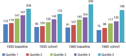
FIGURE 5-6 Average lifetime Social Security benefits for females (in thousands of dollars). Baseline compared with raising the normal retirement age to 70.
SOURCE: Committee generated using Health and Retirement Study data and cohort assumptions.
First, the policy may encourage workers to increase their work effort and delay retirement (behavioral responses that the FEM can incorporate), and this effect may be stronger for top quintile workers than for bottom quintile workers. Second, even if the policy motivates workers in all quintiles to increase work effort by the same amount, the fact that top quintile workers
have a longer life expectancy means that any delays in claiming Social Security benefits will result in a larger gain in lifetime benefits for those workers.
For the 1960 cohort of males, the story is similar: benefits fall by $30,000 (25%) for bottom quintile workers and by $59,000 (20%) for top quintile workers. As a result, the gap between top and bottom quintiles rises from 142 percent to 157 percent of quintile 1 benefits when the NRA is raised. The policy change increases the gap in lifetime benefits by more for the 1960 cohort, as reflected in the fact that the gap between quintiles 1 and 5 grows by 15 percentage points (from 142% to 157%) versus 6 percentage points (from 82% to 88%) for the 1930 cohort.
The results for females, shown in Figure 5-6, are less dramatic with respect to the relative patterns of lifetime benefits. For the 1930 cohort, benefits fall by about 15 percent for quintiles 1 and 5 workers (by $17,000 and $33,000, respectively), leaving the benefit gap ratio between them essentially unchanged (0.86 at baseline and 0.85 after the policy change). The results for the 1960 cohort are more in line with those for males: the relative decline in benefits is larger for quintile 1 (17%) than for quintile 5 (15%), so the gap ratio between quintiles 1 and 5 rises from 158 percent to 164 percent of quintile 1 benefits. The bottom line is that this policy change expands the gap in lifetime benefits by quintile of lifetime earnings.
Total benefits (i.e., including Medicare, Medicaid, and other programs in addition to Social Security) in the baseline and NRA increase scenarios are shown in Figures 5-7 and 5-8 for males and females, respectively. Total benefits at baseline are slightly U-shaped for males in the 1930 cohort; $402,000 for quintiles 1 and 5 males but somewhat lower for males in quintiles 2 through 4. As discussed in Chapter 4, lower-income (lifetime earnings) males receive higher DI, Supplemental Security Income, and Medicaid benefits, while higher-income males receive higher Social Security and Medicare benefits, and these differentials in benefits happen to exactly offset each other for quintiles 1 and 5 males in the base case. For the 1960 cohort, the growth in Social Security and Medicare benefits for high-income workers that is driven by increases in life expectancy changes the pattern so that total benefits rise across the income groups, except that quintile 2 workers continue to have lower benefits than quintile 1 workers.
Because the NRA-increase policy in this simulation reduces Social Security benefits by a larger amount in dollar terms for high-income workers, the U-shaped pattern for the 1930 cohort changes to one where benefits are lower for quintile 5 males than for quintile 1 males. For the 1960 cohort, benefits are still higher for quintile 5 workers than for quintile 1 workers, but the difference ($99,000) is smaller than it was in the baseline scenario with an NRA of 67 ($131,000). Thus, the NRA increase would offset roughly a quarter of the widening gap in benefits between the top and bottom quintiles for the 1930 and 1960 cohorts that is driven by the increase
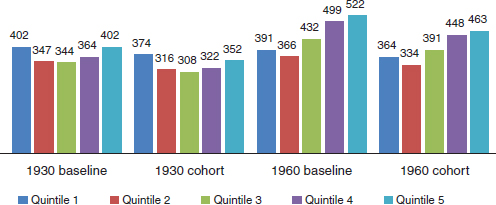
FIGURE 5-7 Average lifetime total benefits for males (in thousands of dollars). Baseline compared with raising the normal retirement age to 70.
SOURCE: Committee generated using Health and Retirement Study data and cohort assumptions.

FIGURE 5-8 Average lifetime total benefits for females (in thousands of dollars). Baseline compared with raising the normal retirement age to 70.
SOURCE: Committee generated using Health and Retirement Study data and cohort assumptions.
in differential life expectancy (because the gap had risen about $130,000 due to life expectancy differences and the policy change would reduce it by about $30,000).
The baseline results for females look a bit different in that total benefits for the 1930 cohort are much larger for quintile 1 workers than for quintile 5 workers, reflecting greater Medicare, Medicaid, DI, and Supplemental
Security Income benefits for low-income females. Because of rising life expectancy, by the 1960 cohort total benefits are larger for the quintile 5 group. Implementing the NRA-increase policy in simulation 2 widens the gap between quintiles 1 and 5 benefits in the baseline scenario. Quintile 1 females in the 1930 cohort have $129,000 more in benefits than quintile 5 females at baseline, but they have $146,000 more than the top quintile under the NRA increase. By contrast, quintile 1 females in the 1960 cohort have $28,000 less than quintile 5 workers at baseline but have only $6,000 less under the NRA-increase scenario. Once again, the NRA increase offsets a portion of the trend toward higher benefits for higher-income workers in later cohorts.
Table 5-2 summarizes these effects of the NRA increase in simulation 2 relative to wealth. Benefits fall across the board, but the decline represents a modestly larger share of baseline wealth for male higher earners than for male lower earners. For females, the decline is noticeably larger for higher earners than lower earners. The differential change between the highest and lowest earnings quintiles is less than 0.5 percentage points for males and almost 2 percentage points for females; the net impact is thus progressive, though with some difference in the pattern for males and females.
Unlike the EEA-increase policy in simulation 1, this policy change would generate substantial savings for the Social Security system. Total
TABLE 5-2 Impact of Raising the Normal Retirement Age to 70
| Present value of net benefits at age 50, relative to wealth, based on the mortality profile for those born in 1960 | |||
| Earnings Quintile | Baseline | Under Policy Experiment | Percentage Point Change |
| Males | |||
|
Lowest |
45.6 |
40.8 |
–4.8 |
|
2 |
36.8 |
31.3 |
–5.5 |
|
3 |
33.3 |
27.7 |
–5.7 |
|
4 |
28.9 |
23.4 |
–5.5 |
|
Highest |
21.4 |
16.2 |
–5.2 |
| Females | |||
|
Lowest |
65.4 |
62.3 |
–3.1 |
|
2 |
54.8 |
50.8 |
–4.0 |
|
3 |
44.9 |
40.2 |
–4.7 |
|
4 |
33.5 |
28.6 |
–4.9 |
|
Highest |
30.8 |
25.9 |
–4.9 |
SOURCE: Committee generated using Health and Retirement Study data and cohort assumptions.
benefit expenditures for males fall by 23 percent, while total benefits for females fall by 15 percent. This simulation therefore suggests that raising the NRA to 70 would enhance the overall solvency of the Social Security system while modestly increasing the progressivity of total benefits.
Policy Simulation 3: Raising Both the EEA and NRA
This simulation essentially combines the first two simulations, enacting a simultaneous increase in the EEA by 2 years and the NRA by 3 years. The results are displayed in Figures 5-9 through 5-12 and Table 5-3. Not surprisingly, the total effect is very similar to what one would obtain by summing the effect of the two reforms individually; because the changes in benefit amounts were much smaller for the EEA increase, the combined effect of the two policies is similar to the effect of the NRA increase alone. This policy reduces benefit expenditures by 22 percent for males and 14 percent for females.
Policy Simulation 4: Reducing Social Security COLAs
Another policy option that has received considerable attention from policy makers is reducing the automatic COLA for Social Security and other benefits. Legislation enacted in 1973 specified that Social Security benefit payments increase every year to keep pace with inflation. The amount of the increase is based on the Consumer Price Index for Urban Wage Earners and Clerical Workers (CPI-W).
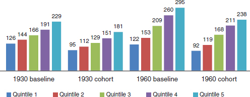
FIGURE 5-9 Average lifetime Social Security benefits for males (in thousands of dollars). Baseline compared with raising the early entitlement age to 64 and the normal retirement age to 70.
SOURCE: Committee generated using Health and Retirement Study data and cohort assumptions.
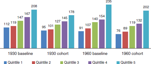
FIGURE 5-10 Average lifetime Social Security benefits for females (in thousands of dollars). Baseline compared with raising the early entitlement age to 64 and the normal retirement age to 70.
SOURCE: Committee generated using Health and Retirement Study data and cohort assumptions.
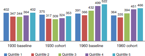
FIGURE 5-11 Average lifetime total benefits for males (in thousands of dollars). Baseline compared with raising the early entitlement age to 64 and the normal retirement age to 70.
SOURCE: Committee generated using Health and Retirement Study data and cohort assumptions.
An alternative proposal is to use the Chained Consumer Price Index for All Urban Consumers (Chained CPI). The Chained CPI takes into account substitutions that consumers make in response to price increases. As a result, the annual increase in the Chained CPI is smaller than the increase in the CPI-W. If Social Security and other benefits were indexed to the Chained CPI, then benefits would grow more slowly over time as retirees age. The
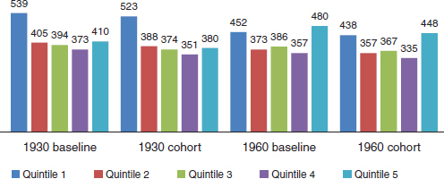
FIGURE 5-12 Average lifetime total benefits for females (in thousands of dollars). Baseline compared with raising the early entitlement age to 64 and the normal retirement age to 70.
SOURCE: Committee generated using Health and Retirement Study data and cohort assumptions.
TABLE 5-3 Impact of Raising the Early Entitlement Age to 64 and the Normal Retirement Age to 70
| Present value of net benefits at age 50, relative to wealth, based on the mortality profile for those born in 1960 | ||||
| Earnings Quintile | Baseline | Under Policy Experiment | Percentage Point Change | |
| Males | ||||
|
Lowest |
45.6 |
40.9 |
–4.8 |
|
|
2 |
36.8 |
31.4 |
–5.5 |
|
|
3 |
33.3 |
27.9 |
–5.5 |
|
|
4 |
28.9 |
23.5 |
–5.3 |
|
|
Highest |
21.4 |
16.3 |
–5.1 |
|
| Females | ||||
|
Lowest |
65.4 |
62.4 |
–3.0 |
|
|
2 |
54.8 |
50.9 |
–3.9 |
|
|
3 |
44.9 |
40.4 |
–4.5 |
|
|
4 |
33.5 |
28.8 |
–4.7 |
|
|
Highest |
30.8 |
26.1 |
–4.7 |
|
SOURCE: Committee generated using Health and Retirement Study data and cohort assumptions.
FIGURE 5-13 Average lifetime Social Security benefits for males (in thousands of dollars). Baseline compared with reducing real benefits by 0.2 percent annually.
SOURCE: Committee generated using Health and Retirement Study data and cohort assumptions.
impact of this change compounds over time, so groups with longer life expectancies would be more affected.
To simulate the impact of switching from the CPI-W to a Chained CPI, this simulation reduces real benefits by 0.2 percent annually, in contrast to the baseline scenario where benefits rise to keep pace with inflation.7 The effect of this change on Social Security benefits for males can be seen in Figure 5-13. Benefits fall for all quintiles, but the drop is larger on average for the higher income quintiles, as expected because of their longer life expectancy. For the 1930 cohort, benefits fall by $3,000 for quintile 1 and by $6,000 for quintile 5. For the 1960 cohort, benefits fall by $3,000 for quintile 1 and by $9,000 for quintile 5. These declines translate into relatively small changes in the gap between highest and lowest quintiles as a share of quintile 1 benefit, which falls from 0.82 to 0.81 for the 1930 cohort and from 1.42 to 1.40 for the 1960 cohort.
The effect for females, shown in Figure 5-14, is very similar to that for males; there is a larger drop in benefits for quintile 5 than for quintile 1, but the dollar amounts are small. The effect on total benefits, shown in Figures 5-15 and 5-16, is quite similar to the effect for Social Security only. Table 5-4 shows the impact relative to wealth; on average, net benefits fall by a larger share of wealth for top earners than lower earners, but the effect is relatively small. The overall impact is thus to make entitlement benefits slightly more progressive.
________________
7In reality, the impact of the policy change would depend on the difference in the future between the Chained CPI and CPI-W. That difference has been smaller over the past 2 years than 20 basis points.
FIGURE 5-14 Average lifetime Social Security benefits for females (in thousands of dollars). Baseline compared with reducing real benefits by 0.2 percent annually.
SOURCE: Committee generated using Health and Retirement Study data and cohort assumptions.
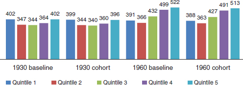
FIGURE 5-15 Average lifetime total benefits for males (in thousands of dollars). Baseline compared with reducing real benefits by 0.2 percent annually.
SOURCE: Committee generated using Health and Retirement Study data and cohort assumptions.
The effect of the policy on system finances is similarly modest, because it reduces program expenditures by about 2 percent. In terms of thinking about how this policy affects individual retirees, it is worth remembering that the values reported here are averages for the cohort. Those individuals who end up being particularly longer lived will experience larger decreases in benefits than the average. There are more of these individuals in higher-income groups, and so the average drop in benefits is larger for these groups, but there will be individuals in every quintile who experience large drops in benefits as a result of this policy.

FIGURE 5-16 Average lifetime total benefits for females (in thousands of dollars). Baseline compared with reducing real benefits by 0.2 percent annually.
SOURCE: Committee generated using Health and Retirement Study data and cohort assumptions.
TABLE 5-4 Impact of Reducing Real Benefits by 0.2 Percent Annually
| Present value of net benefits at age 50, relative to wealth, based on the mortality profile for those born in 1960 | ||||
| Earnings Quintile | Baseline | Under Policy Experiment | Percentage Point Change | |
| Males | ||||
|
Lowest |
45.6 |
45.2 |
–0.4 |
|
|
2 |
36.8 |
36.3 |
–0.5 |
|
|
3 |
33.3 |
32.7 |
–0.6 |
|
|
4 |
28.9 |
28.2 |
–0.7 |
|
|
Highest |
21.4 |
20.8 |
–0.6 |
|
| Females | ||||
|
Lowest |
65.4 |
65.1 |
–0.2 |
|
|
2 |
54.8 |
54.4 |
–0.3 |
|
|
3 |
44.9 |
44.5 |
–0.4 |
|
|
4 |
33.5 |
33.1 |
–0.4 |
|
|
Highest |
30.8 |
30.3 |
–0.5 |
|
SOURCE: Committee generated using Health and Retirement Study data and cohort assumptions.
Policy Simulation 5: Reducing the Top PIA Factor to 10 Percent
The final two policy simulations reduce benefits in ways that primarily affect higher-income workers. As previously noted, many proposals designed to restore the Social Security program to long-term solvency involve
some kind of benefit cut; there may be political support for reducing benefits in a way that protects lower-income workers, because lower-income older households on average rely on Social Security for a large share of their retirement income. A second rationale for enacting benefit reductions in this way is that the reductions might offset some of the decrease in benefit progressivity that is occurring naturally because of rising inequality in life expectancy.
The first such policy simulated by the committee changes the replacement rate on the third leg of the AIME-to-PIA conversion formula from 15 to 10 percent. Thus, each dollar of the AIME beyond the second bend point (currently $4,917 of monthly earnings) would provide only an additional 10 cents of monthly Social Security benefit, instead of an additional 15 cents as under the current formula.
The results of this policy-change simulation are shown in Figures 5-17 and 5-18 for males and females, respectively. For the 1930 cohort, Social Security benefits fall by $1,000 for males in quintiles 3 and 4 and by $3,000 for quintile 5 males; benefits for males in quintiles 1 and 2 are unaffected. The effect for the 1960 cohort is slightly larger: $2,000 for quintile 4 and $4,000 for quintile 5. The effects for females are much smaller because of their lower average earnings: Social Security benefits fall by $1,000 for quintile 5 but are otherwise unchanged. The effect on total benefits, seen in Figures 5-19 and 5-20, is essentially the same, a drop of at most $4,000 for workers in the top quintile. Thus, this policy change is too modest to offset much of the increase in benefits accruing to higher-income workers in the 1960 cohort as a result of their longer life expectancy. Table 5-5 shows the
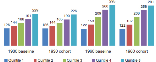
FIGURE 5-17 Average lifetime Social Security benefits for males (in thousands of dollars). Baseline compared with reducing the top primary insurance amount factor by one-third.
SOURCE: Committee generated using Health and Retirement Study data and cohort assumptions.
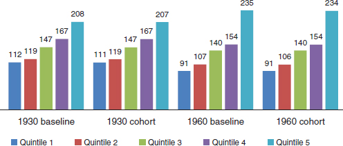
FIGURE 5-18 Average lifetime Social Security benefits for females (in thousands of dollars). Baseline compared with reducing the top primary insurance amount factor by one-third.
SOURCE: Committee generated using Health and Retirement Study data and cohort assumptions.
impact relative to wealth; net benefits fall by a slightly larger proportion of wealth for higher earners than lower earners, so the impact is slightly progressive. The savings to the Social Security system are similarly modest, less than 1 percent of program expenditures.
Policy Simulation 6: Lower Initial Benefits for Top 50 Percent of Earners
The final Social Security policy change simulated for the committee’s analysis is intended to reduce benefits to workers in the top half of the AIME distribution. It moves the second bend point in the AIME-to-PIA formula (currently $4,917) to the median level of the AIME and changes the replacement rate for income beyond the second bend point from 15 percent to zero. Thus, this policy should have at least three times the effect of simulation 5, because it reduces the replacement rate above the second bend point all the way to zero rather than just to 10 percent, plus an additional effect from moving the bend point itself.
The effects of this policy on Social Security benefits for males and females are shown in Figures 5-21 and 5-22, respectively. This policy lowers benefits for quintile 1 males in the 1930 cohort by $8,0008 but lowers them
________________
8To understand how this is possible, recall that our income measure is the average of nonzero earnings at ages 41 to 50, whereas benefits are based on lifetime earnings. Also, the quintiles in this analysis are based on household incomes, whereas the benefits are based on individual earnings.
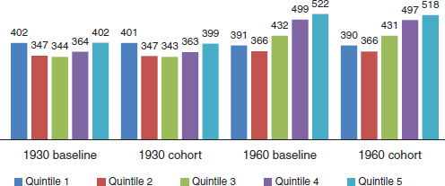
FIGURE 5-19 Average lifetime total benefits for males (in thousands of dollars). Baseline compared with reducing the top primary insurance amount factor by one-third.
SOURCE: Committee generated using Health and Retirement Study data and cohort assumptions.
FIGURE 5-20 Average lifetime total benefits for females (in thousands of dollars). Baseline compared with reducing the top primary insurance amount factor by one-third.
SOURCE: Committee generated using Health and Retirement Study data and cohort assumptions.
by much more for higher-income males: Quintiles 4 and 5 males experience a drop in lifetime benefits of $23,000 and $38,000, respectively. The fall in benefits is even larger for men in the 1960 cohort, where quintiles 4 and 5 males now see benefits fall by $32,000 and $49,000, respectively. Effects for females are smaller, as might be expected because of their lower earnings. Quintile 5 females experience a $14,000 decline in benefits in both the 1930 and 1960 cohorts.
TABLE 5-5 Impact of Reducing the Top PIA Factor by One-Third
| Present value of net benefits at age 50, relative to wealth, based on the mortality profile for those born in 1960 | ||||
| Earnings Quintile | Baseline | Under Policy Experiment | Percentage Point Change | |
| Males | ||||
|
Lowest |
45.6 |
45.6 |
–0.1 |
|
|
2 |
36.8 |
36.8 |
–0.1 |
|
|
3 |
33.3 |
33.2 |
–0.1 |
|
|
4 |
28.9 |
28.7 |
–0.2 |
|
|
Highest |
21.4 |
21.1 |
–0.3 |
|
| Females | ||||
|
Lowest |
65.4 |
65.4 |
0.0 |
|
|
2 |
54.8 |
54.8 |
0.0 |
|
|
3 |
44.9 |
44.8 |
–0.1 |
|
|
4 |
33.5 |
33.4 |
–0.1 |
|
|
Highest |
30.8 |
30.7 |
–0.1 |
|
SOURCE: Committee generated using Health and Retirement Study data and cohort assumptions.
The effects on total benefits can be seen in Figures 5-23 and 5-24. The most interesting aspect of these figures is how the policy change helps to offset the increase in benefits resulting from rising inequality in life expectancy. For males in the 1930 cohort, total benefits for quintiles 1 and 5 in the baseline scenario are the same, while for the 1960 cohort, benefits in the baseline scenario are $131,000 higher in quintile 5 than quintile 1. Thus, a gap between top and bottom quintiles of $131,000 emerges between these two cohorts in the baseline scenario. If this policy were implemented, then the gap between the top and bottom quintiles for the 1960 cohort would be only $90,000, or 70 percent as large. For females, the gap between the top and bottom quintiles is $28,000 for the 1960 cohort at baseline, versus $16,000 under the simulated policy change.
Table 5-6 shows the change in net benefits relative to wealth. The decline is much larger for higher earners than lower earners, so the effect is to make overall benefits from the entitlement programs examined in this analysis more progressive. Note that for males in the top quintile of lifetime earnings, the effect of the policy is to reduce net benefits by 3.4 percent of inclusive wealth. This is about half the gain enjoyed by this group of earners (6.9 percent of wealth) from the steeper mortality gradient between the 1930 and 1960 cohorts.
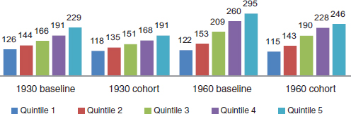
FIGURE 5-21 Average lifetime Social Security benefits for males (in thousands of dollars). Baseline compared with reducing benefits to workers in the top half of the average indexed monthly earnings distribution.
SOURCE: Committee generated using Health and Retirement Study data and cohort assumptions.
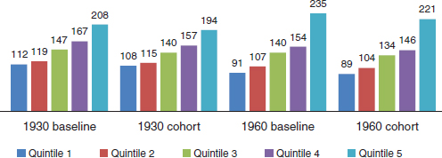
FIGURE 5-22 Average lifetime Social Security benefits for females (in thousands of dollars). Baseline compared with reducing benefits to workers in the top half of the average indexed monthly earnings distribution.
SOURCE: Committee generated using Health and Retirement Study data and cohort assumptions.
This policy change generates much larger savings for the Social Security system than the policy change in simulation 5. Benefit expenditures fall by 11 percent for males and by 5 percent for females.
Box 5-5 considers another approach to offsetting the differential effects on lifetime benefits by quintile, one which would apply different factors to workers who defer claiming benefits depending on their position within the lifetime earnings distribution.
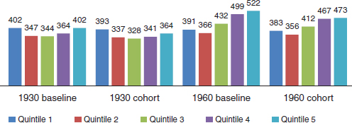
FIGURE 5-23 Average lifetime total benefits for males (in thousands of dollars. Baseline compared with reducing benefits to workers in the top half of the average indexed monthly earnings distribution.
SOURCE: Committee generated using Health and Retirement Study data and cohort assumptions.
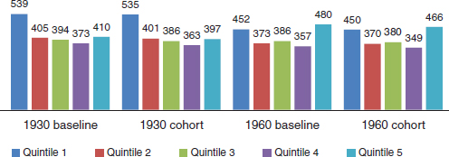
FIGURE 5-24 Average lifetime total benefits for females (in thousands of dollars). Baseline compared with reducing benefits to workers in the top half of the average indexed monthly earnings distribution.
SOURCE: Committee generated using Health and Retirement Study data and cohort assumptions.
A MEDICARE POLICY SIMULATION: RAISING THE ELIGIBILITY AGE FOR MEDICARE
Medicare faces long-term fiscal imbalances that result from both population aging and rapidly rising per capita health care spending. As with Social Security, these fiscal imbalances likely will lead policy makers to consider various options to improve Medicare financing. One option that has been discussed is to raise the usual eligibility age for Medicare from 65 to 67 (Congressional Budget Office, 2013a). When Social Security and
TABLE 5-6 Lower Initial Social Security Benefits for Top Half of Earners (by average indexed monthly earnings)
| Present value of benefits at age 50, relative to present value of consumption, based on the mortality profile for those born in 1960 | ||||
| Earnings Quintile | Baseline | Under Policy Experiment | Percentage Point Change | |
| Males | ||||
|
Lowest |
45.6 |
44.5 |
–1.1 |
|
|
2 |
36.8 |
35.4 |
–1.4 |
|
|
3 |
33.3 |
31.2 |
–2.1 |
|
|
4 |
28.9 |
26.2 |
–2.7 |
|
|
Highest |
21.4 |
18.0 |
–3.4 |
|
| Females | ||||
|
Lowest |
65.4 |
65.1 |
–0.3 |
|
|
2 |
54.8 |
54.3 |
–0.5 |
|
|
3 |
44.9 |
44.0 |
–0.9 |
|
|
4 |
33.5 |
32.4 |
–1.1 |
|
|
Highest |
30.8 |
29.5 |
–1.3 |
|
SOURCE: Committee generated using Health and Retirement Study data and cohort assumptions.
Medicare were enacted, the age of eligibility was 65 for both programs. Since then, the normal retirement age for Social Security has been increased to 67, whereas the usual Medicare age has remained unchanged.9
Some Medicare beneficiaries, however, qualify for Medicare by virtue of being disabled, rather than at age 65, and they would not be affected by a change in “usual” Medicare eligibility age.10 In addition, were the Medicare eligibility age to change, some 65- and 66-year-olds would become eligible for health insurance subsidies under the new Affordable Care Act11 health exchanges. However, because the FEM is calibrated with data preceding the enactment of the Affordable Care Act, the simulation performed by the committee (simulation 7) does not capture this possibility.
_________________________
9One significant difference between Medicare and Social Security, however, is that Medicare provides an in-kind benefit, health insurance, that at least prior to the implementation of the Affordable Care Act, was difficult to purchase on the private market, particularly for those with preexisting health conditions.
10In particular, Medicare is available to people under age 65 with end-stage renal disease and to those who have been eligible for Social Security disability benefits for at least 2 years.
11As noted in Chapter 2, the formal name of the legislation is the Patient Protection and Affordable Care Act of 2010.
BOX 5-5
Differential Increases in Subsequent Benefits
Based on Average Indexed Monthly Earnings
Social Security encourages people to defer claiming their benefits by raising the annual benefit level for those who delay claiming beyond their early entitlement age. The goal of this system is to keep lifetime benefits approximately constant regardless of the age at claiming, so the higher benefit at, say, age 67 is intended to offset (in expected present value) the effect of not receiving benefits at ages 62 through 67.
Social Security implements this approach through early retirement adjustments and the Delayed Retirement Credit. For workers who claim benefits before their normal retirement age (NRA), the benefit level is reduced by 6.67 percent for each year up to 3 years prior to the NRA, and then 5 percent for each additional year thereafter. So if the benefit level at the NRA is $10,000 per year and the NRA is 67, then the annual benefit for a worker who claims at age 62 is $7,000 and the annual benefit for a worker who claims at age 64 is $8,000. The extra $3,000 and $2,000, respectively, per year for waiting to claim until age 67 is intended to offset the present value impact of not receiving benefits until that age.
For those who defer claiming their benefits until after their NRA, Social Security has a similar goal, but a different mechanism (the Delayed Retirement Credit) for implementing the adjustment. For workers born in 1943 or later, Social Security raises the annual benefit level by 8 percent for each year of delayed claiming beyond the NRA, up to age 70. So if the normal retirement age is 67 and the benefit level at that age is $10,000 per year, then a worker who delays claiming until age 70 would receive $12,400 per year.
Both the adjustment prior to the NRA and the Delayed Retirement Credit are intended to keep the present value of lifetime benefits roughly constant, on average, for workers who claim benefits at different ages. Yet, as this report has documented, life expectancies vary systematically from the average, and the gap in life expectancies for identifiable groups by income and education has been expanding. The result of these differences is that even if the system is roughly actuarially neutral on average, workers in low earnings categories who defer claiming their benefits will tend to experience a reduction in the present value of their lifetime benefits (because their life expectancy is lower than average), as will workers in high earnings categories who claim their benefits early (for the opposite reason). These effects are becoming larger as the gap in life expectancy between lower and higher earners increases.
In theory, the differential effects on lifetime benefits by earnings quintile could be offset by applying different factors to workers who defer claiming benefits, depending on their position within the lifetime earnings distribution. For example, one could calculate the adjustment factor by quintile that would keep lifetime benefits constant across claiming age, given the mortality projections for workers in that quintile. In practice, as with a structure of adjusting initial benefit levels for differential life expectancy experience, some smoothing process would be required to avoid big jumps in adjustment factors immediately below and above the quintile thresholds; it may also be desirable to give workers nearing retirement certainty about the benefit structure they will face in retirement.
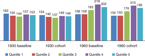
FIGURE 5-25 Average lifetime Medicare benefits for males (in thousands of dollars). Baseline compared with raising the Medicare eligibility age to 67.
SOURCE: Committee generated using Health and Retirement Study data and cohort assumptions.
The results for the committee’s simulation of how this policy change would affect lifetime Medicare benefits for males and females are shown in Figures 5-25 and 5-26, respectively. Overall, the delay in eligibility age has a very small effect on lifetime Medicare benefits, mostly because health spending at ages 65 and 66 is quite low relative to later in life. The effect is only a bit larger for those in the lowest-income groups. Although these beneficiaries have significantly higher Medicare spending at ages 65 and 66 and significantly lower life expectancy, both of which increase the effect on lifetime benefits, they are also more likely to qualify for Medicare through their disability status and hence be unaffected by the policy change.
For example, for males in the 1930 cohort, those in quintile 1 lose $8,000 in lifetime benefits when the eligibility age is delayed, compared to a loss of $7,000 for those in quintile 5. The differences are somewhat larger for females, particularly in the 1960 cohort. For this cohort, the increase in the Medicare eligibility age decreases lifetime Medicare benefits by $11,000 for females in quintile 1 and by $7,000 for females in quintile 5.
Table 5-7 shows the results relative to wealth. The decline in net benefits for the lowest quintile is 0.8 to 0.9 percentage points of wealth larger than for the highest quintile. The result is thus regressive.
SUMMARY OF RESULTS FROM THE POLICY SIMULATIONS
This chapter presented seven simulated policy experiments that have an impact on the receipt of lifetime benefits from various entitlement programs. Table 5-8 summarizes some of these effects in terms of how a given policy change affects (1) progressivity, given the health and mortal-
FIGURE 5-26 Average lifetime Medicare benefits for females (in thousands of dollars). Baseline compared with raising the Medicare eligibility age to 67.
SOURCE: Committee generated using Health and Retirement Study data and cohort assumptions.
TABLE 5-7 Impact of Raising the Medicare Eligibility Age to 67
| Present value of benefits at age 50, relative to present value of consumption, based on the mortality profile for those born in 1960 | ||||
| Earnings Quintile | Baseline | Under Policy Experiment | Percentage Point Change | |
| Males | ||||
|
Lowest |
45.6 |
44.2 |
–1.4 |
|
|
2 |
36.8 |
35.7 |
–1.1 |
|
|
3 |
33.3 |
32.5 |
–0.8 |
|
|
4 |
28.9 |
28.2 |
–0.7 |
|
|
Highest |
21.4 |
20.9 |
–0.5 |
|
| Females | ||||
|
Lowest |
65.4 |
63.9 |
–1.5 |
|
|
2 |
54.8 |
53.3 |
–1.5 |
|
|
3 |
44.9 |
43.5 |
–1.4 |
|
|
4 |
33.5 |
32.3 |
–1.2 |
|
|
Highest |
30.8 |
30.1 |
–0.7 |
|
SOURCE: Committee generated using Health and Retirement Study data and cohort assumptions.
TABLE 5-8 Progressivity of Policy Options for Improving the Solvency of Social Security and Medicare: Effect on Present Value of Benefits Relative to Consumption for Top and Bottom Quintiles Based on Average Indexed Monthly Earnings
| Policy Experiment | Impact on Progressivity | Impact on Present Value of Net Benefits Relative to Wealth for Bottom/ Top Quintiles for Males | Impact on Solvency |
| Raise EEA from age 62 to 64 | Somewhat less progressive | +0.1 | Small |
| +0.4 | |||
| Raise NRA to age 70 | Somewhat more progressive | −4.8 | Significant (23% reduction in present value benefits for males; 15% reduction for females) |
| −5.2 | |||
| Raise EEA and NRA as above | Somewhat more progressive | −4.8 | Significant (22% reduction in benefits for males; 14% for females) |
| −5.1 | |||
| COLA based on chained CPI | Somewhat more progressive | −0.4 | Small (reduces benefits by less than 2%) |
| −0.6 | |||
| Marginal benefit 10% at top | Somewhat more progressive | −0.1 | Small (reduces benefits by less than 1%) |
| −0.3 | |||
| Marginal benefit after median | Substantially more progressive | –1.1 | Medium (11% reduction in benefits for males, 5% for females) |
| –3.4 | |||
| Raise Medicare eligibility to age 67 | Less progressive | –1.4 | Modest (in part because 65- and 66-year-olds are much less expensive than older beneficiaries, and in part because some would qualify through disability insurance) |
| –0.5 | |||
NOTE: COLA = cost-of-living adjustment, CPI = consumer price index, EEA = early entitlement age, NRA = normal retirement age.
SOURCE: Committee generated using Health and Retirement Study data and cohort assumptions.
ity experience of people born in 1960 and (2) the solvency of the current Social Security (for simulations 1 through 6) or Medicare (simulation 7) systems.
ANNEX TO CHAPTER 5: THE COMMITTEE’S RETIREMENT MODEL
Predicting when people are going to retire and how those decisions might change in response to various policy changes is a challenging modeling exercise. In this annex the committee provides a nontechnical overview of its approach, explains the merits of this approach compared to alternatives in the retirement literature, and provides some indication of the sensitivity of the results to its choice of approach.
The approach adopted in this report for predicting retirement choices is based on what economists call a “reduced-form model.” To estimate such a model, the analyst first identifies an outcome of interest and all of the variables that might be expected to influence that outcome. To be specific, we defined our outcome to be employment, which allows us to analyze situations in which individuals may return to as well as exit from employment. The explanatory variables in the model include age, sex, AIME quintile, and health variables, as well as whether the individual was working during the previous 2 years. The data we use to estimate this model come from the HRS, a longitudinal panel survey that interviews individuals aged 50 and older every 2 years.
The model is estimated via statistical methods in which the projected relationship between each explanatory variable and employment is chosen so that the model as a whole predicts actual employment behavior as closely as possible. To give a flavor of the results, the model finds, for example, that a male is 5 percentage points more likely to be working than a female and that someone who was working 2 years ago is 60 percentage points more likely to be working currently than someone who was not.
Reduced-form models such as this one are commonly used in economic analyses of retirement behavior. They have been used, for example, to study the effect of financial incentives from Social Security and private pensions, health and health insurance, and wealth and unemployment (see, e.g., National Research Council, 1996; Gustman and Steinmeier, 2002; Belloni, 2008; Chetty, 2008). Such models essentially estimate correlations between each factor and the outcome of interest, holding the other factors constant. Despite their popularity, however, they are subject to critique. One critique pertains to the validity of the results. If the analyst fails to include in the model all the factors that might affect the outcome measure, then the estimates may be biased, although the best studies are careful to use strategies to mitigate this concern. A more fundamental concern, perhaps, is that a
reduced-form model is by its nature “atheoretical,” in the sense that the model simply measures the connection between variables, say age and work. It does not uncover the underlying drivers of that connection, such as the discount rate: the rate at which individuals would be willing to trade off between income today and income in the future.
An alternative approach is to estimate a “structural model.” In this approach, the analyst writes down an equation (or system of equations) that he or she believes is an appropriate characterization of how individuals approach a decision such as retirement, with only a few unknown parameters such as the discount rate. The analyst then uses datasets such as the HRS to estimate the parameter values that will make predicted behavior match observed behavior as closely as possible. The advantage of such an approach is that the process generates estimates of parameters such as the discount rate, which may be valuable if the analyst wants to do a simulation well outside the range of actual experience, such as how retirement behavior would change if Social Security were eliminated.12 Proponents of this approach point out that while reduced-form models generally must include age indicator variables to be able to explain the tendency of people to retire at ages such as the Social Security EEA and NRA, a structural model can explain this behavior without them.13 On the other hand, the validity of structural estimation fundamentally rests on whether the analyst has correctly specified the relationships governing individual behavior, an assumption that cannot be formally tested, and must rather be assessed in relation to theory, the plausibility of the resulting parameter estimates, and the ability of the estimated model to make plausible predictions of responses to change.
_________________________
12For large changes (such as eliminating Social Security altogether), the structural form estimate is only valuable in this way if the underlying parameter would remain unchanged. It is possible, however, to imagine that the underlying parameter varies in some way; if that variation occurs outside the observed data, then it is unlikely the structural form estimation will reflect it.
13One natural question that may occur with the committee’s approach is how we treat the “excess” tendency to retire at the EEA and NRA in policy simulations where those ages are changed. In our model, the age indicators are defined relative to the EEA and NRA, not to actual ages. So for example, an individual in the simulation who is age 62 and who faces a NRA of 67 will have a value of 1 for the “at EEA” age indicator and a value of 1 for the “5 years before NRA” indicator. In a policy simulation that moves the EEA to age 64 but leaves the NRA unchanged, this individual’s EEA indicator is reset to zero because he is no longer at the EEA; another individual who is age 64 would have her “at EEA” indicator set to 1. Beecause the model estimates reflect that people are less likely to work once they reach the EEA, this change will tend to raise the probability that the age-62 individual is working and lower the probability that the age-64 individual is working, relative to the base case. To the extent that 62-year-olds retire at age 62 for reasons other than their proximity to the EEA and NRA, this approach will tend to overstate the change in retirement behavior that will result from this policy change.
A number of authors have popularized the use of structural estimation in the retirement context, including Gustman and Steinmeier (1986), Rust and Phelan (1997), French (2005), and Van der Klaauw and Wolpin (2008). The authors of these studies generally validate their model based on its ability to generate reasonable parameter estimates and to match known features of retirement behavior, like the increased tendency to retire at the EEA and NRA. In many cases, authors also use their models to project the effect of changes to Social Security or other government policies on retirement behavior.
Although in theory it is appealing to use results from these studies to validate the committee’s policy simulations, challenges emerge in practice. First, the results from different studies are not always consistent with each other. For example, Gustman and Steinmeier (2005) predict that raising the EEA to 64 would cause many people to delay retirement from age 62 to 64, while French (2005) estimates that increasing the EEA would have little effect on retirement. Also, the policy simulations may not be identical to those used for this report. Gustman and Steinmeier (2009), for example, simulate the effect of recent changes to Social Security, including the increase in the NRA, increase in the Delayed Retirement Credit (which raises the value of delays in claiming Social Security), and elimination of the earnings test for early claiming years prior to the NRA, but they do not report the effect of these changes separately, as would be necessary for comparison to the simulations presented here.
There are other ways of assessing whether the committee’s approach is likely to generate reliable estimates of the effect of policy change. First, one can explore how well our model’s predictions match observed real-world behavior. We begin by calculating employment rates and rates of Social Security receipt for males and females in the 1930 birth cohort using data from the 1980-2010 March Current Population Surveys (CPS) of the U.S. Census Bureau.14
We then predict these same outcome measures using our models (the employment model described above and analogous reduced-form models for claiming of Social Security retired worker and DI benefits). The results from our models, along with the CPS data, are presented in Figure 5-27 shows that Social Security receipts as predicted from our models match reasonably well with actual receipts
________________
14See https://www.census.gov/mp/www/cat/people_and_households/current_population_survey.html [July 2015].
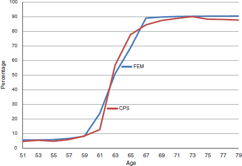
FIGURE 5-27 Percentage of 1930 cohort receiving Social Security benefits, by age. Estimates from the Future Elderly Model and the 1980-2010 March Current Population Surveys.
SOURCE: Committee generated using Health and Retirement Study data, data from the 1980-2010 March Current Population Surveys, and cohort assumptions.
as reported in the CPS.15Figure 5-28 shows that our models predict a somewhat higher share of the population working at any given age relative to that observed in the CPS (the average difference is about 5 percentage points), but the pattern of employment decline by age is similar in the two series.
Finally, one can explore how the model behaves “out of sample” by looking more closely at how working and claiming behavior are projected to change in one of this report’s policy simulations. Figure 5-29 compares receipt of Social Security benefits (retired worker benefits and DI benefits) under the base case scenario and in simulation 2, in which the NRA is raised from 67 to 70. The model projects that this policy change would lead to significant delays in claiming relative to the baseline scenario—for example, the age at which half of the sample has claimed rises by 3 years,
________________
15The committee’s model estimates transition over a 2-year period (corresponding to one survey wave), so a spike in behavior that occurs at age 62 in the real world may end up being partly reflected in the age 61 value and partly in the age 63 value in that model.
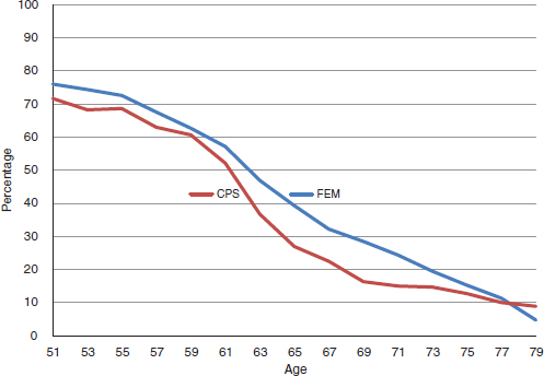
FIGURE 5-28 Percentage of 1930 cohort employed, by age, Future Elderly Model baseline scenario versus raising the normal retirement age to age 70.
SOURCE: Committee generated using Health and Retirement Study data, data from the 1980-2010 March Current Population Surveys, and cohort assumptions.
from age 62 to 65. This is broadly consistent with results reported by Song and Manchester (2008), who found that the increase in the NRA from 65 to 66 was associated with declines in the probability of claiming at ages 62 to 64, and with Behaghel and Blau (2012), who found that the spike at age 65 in the claiming hazard migrated to follow the NRA. Figure 5-30 shows employment under the committee’s baseline and NRA increase (simulation 2) scenarios. The increase in the NRA leads to increases in employment, but the gap between the base case and policy simulation is smaller than in Figure 5-29. This difference is in line with Mastrobuoni (2009), who found that the increase in NRA from age 65 to 66 led the age of retirement claiming to increase by about half as much.
Despite the broad consistency between the results presented here for this specific policy change and other published results, it remains true that the results generated from any model should be treated with caution when assessing the effects of policy changes. Such caution is particularly warranted for results from reduced-form models, such as the one used in this report, because the behavioral response to a policy change may differ from the correlations embodied in the historical data used to estimate the model.
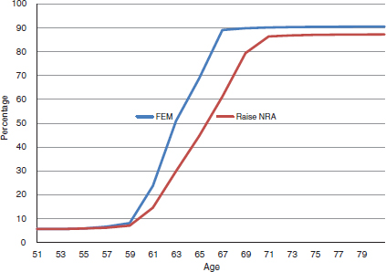
FIGURE 5-29 Receipt of Social Security benefits, by age, Future Elderly Model baseline scenario versus raising the normal retirement age to age 70.
SOURCE: Committee generated using Health and Retirement Study data and cohort assumptions.
FIGURE 5-30 Percentage of 1930 cohort employed, by age, Future Elderly Model baseline scenario versus raising the normal retirement age to age 70.
SOURCE: Committee generated using Health and Retirement Study data and cohort assumptions.


