
3
Growing Heterogeneity of
the U.S. Population in Income
and Life Expectancy
Income inequality has risen noticeably in the United States over the past three decades. According to the Congressional Budget Office (CBO), the share of pretax aggregate household income accruing to households in the bottom quintile of the income distribution fell from 6.2 percent in 1979 to 5.1 percent in 2010 (Congressional Budget Office, 2013b). Over that same period, the share accruing to households in the top quintile rose from 44.9 percent to 51.9 percent—and the share accruing to households in the top 1 percent of the distribution rose from 8.9 percent to 14.9 percent.
The leading view among economists is that skills-biased technical change and the evolution of educational levels have combined to play the leading role in income and earnings inequality. Although the demand for skilled labor has continued to expand over time, the rise in educational attainment has slowed (Goldin and Katz, 2010). The result has been a higher return to education, which has caused an increase in earnings inequality.
Underlying the changes in demand for skills are technology and globalization. In recent decades, transportation and communication costs have fallen and capital has become more mobile. Although consumers have benefited from lower prices, workers in advanced economies are facing greater competition from low-wage countries, which may affect wages (Autor et al., 2013). Indeed, by exploring cross-industry data, a recent Brookings analysis found that out of the 3.9 percentage point decline in labor’s share of income over the past 25 years, import competition may account for 3.3 percentage points (Elsby et al., 2013).
Technology and globalization caused “job polarization” (particularly in the 1990s) where employment growth was concentrated in “high-skill,
high-wage” and “low-skill, low-wage” jobs. “Middle-skill” jobs, such as bookkeeping and clerical work, suffered (Autor, 2010). More recently, however, within-occupation inequality has grown more than between-occupation inequality, which is not what would be expected if technical change were the main cause (Mishel et al., 2013). Some economists have therefore started to examine other institutional factors, including the decline in labor unions (Western and Rosenfeld, 2011) and the tax system (Piketty, 2013).
The causes and consequences of this evolution in the distribution of household income have been widely debated and studied, and policy makers appear to be well aware of the tradeoffs involved in different approaches to offsetting the rise in income inequality through tax and benefit programs. For this reason, the committee chose to focus on a dimension of inequality that has received less attention: that is, how life expectancies have changed for people with different education and income levels.
For policy purposes, the widening longevity dispersion by income category1 is highly relevant because benefits in some programs such as Social Security are linked to long-term income. The full value of those benefits, measured as a present value of expected future benefits received, depends on how long the beneficiaries are expected to live. The growing mortality differences across income can make the benefit structures less progressive (or more regressive) on a lifetime basis.
This chapter discusses the literature on differences in mortality by education and income and then presents the committee’s own estimates that will be used for the policy simulations in later chapters. What matters for the effect of mortality on the distribution of benefits is the association of mortality with long-term earnings. It is important that this association be relatively unaffected by cases in which temporary ill health causes a concurrent loss of earnings and also an increase in mortality.2 Cases of this
________________
1While the dispersion of earnings and incomes has widened in the United States, the dispersion in age at death for adults (deaths after age 10) has actually narrowed (Edwards, 2011). Despite this narrowing, many studies have found that mortality differences by educational attainment have widened, and likewise by position in the earnings distribution. These findings may seem inconsistent with the narrowing of the dispersion of age at death, but in fact need not be if the increase in differences among education and income groups is offset by a reduction in differences within these groups. Lest this appear unlikely, the committee notes that it is exactly what happened with total world inequality in age at death: within-country differences fell, while between-country differences rose, leaving the total inequality almost unchanged from 1970 to 2000 (Edwards, 2013). This is also what Bound and colleagues (2014) found for the United States with respect to mortality inequality within quantile education groups and overall. Sasson (2014) reports complicated patterns of change in the dispersion of age at death within education groups.
2In this case, the resulting association would arise from a short-term reduction in earnings due to illness and would not reflect an association of mortality with the long-term earnings level that would in turn determine benefit levels.
sort will be largely, though not entirely, avoided by analyzing mortality in relation to long-term earnings. The committee measures long-term earnings as the average of nonzero earnings at ages 41 to 50 years.
SHIFT IN THE MORTALITY GRADIENT AND UNDERLYING CAUSES
There is a long tradition of studying differences in mortality by various measures of socioeconomic status (SES) in the United States. A longevity advantage for higher SES groups has been well established in the literature, and sizable differentials in mortality have been documented for more than 40 years (see, for example, Kitagawa and Hauser, 1973). More recent research has found that the differences in mortality not only persist today but also have widened substantially. This research has taken three different approaches. One looks at differences in the mortality of populations of U.S. counties in relation to county-level economic measures. Another looks at mortality by educational attainment. A third approach looks at mortality by career earnings. All three approaches find that the mortality differences are widening.
By whichever indicator is used to capture SES, the evidence shows clearly that since 1960, there has been a large increase in the United States in differential mortality (see, for example, Pappas et al., 1993, using data for 1960-1986). Disparities in mortality have risen whether income or educational achievement is used as the indicator of SES (Preston and Elo, 1995; Manchester and Topoleski, 2008).
The prevailing view among scholars is that mortality differentials originate in part in early childhood or in utero and in part in the health-related behaviors and outcomes of individuals spread over their later life course (Almond and Currie, 2011; Montez and Hayward, 2011). Health-related behaviors (in particular smoking and the nutrition and physical activity lifestyles related to obesity), as well as access to health care, cognitive functioning, and the development of social and psychological resources to seek and preserve health, are the major sources of the mortality differentials. Health behaviors are estimated to account for about 30 percent of the mortality difference for individuals with high versus low levels of education (see summary of the causes for the relation between educational achievement and mortality in Hummer and Hernandez, 2013).
Of particular relevance for the work of this committee is the significant role attributed to smoking and obesity; these two health behaviors/conditions account for a large share of the adult-age mortality disparities across SES groups. Fenelon and Preston (2012) document that overall, about one-fifth of deaths among men and women were attributable to smoking in 2004, and smoking-related mortality explains a large fraction (60 percent)
of the U.S. mortality differences across states, specifically the southern states compared to other regions (Fenelon and Preston, 2012). Despite a recent decline in the prevalence of smoking in the United States, the contribution of smoking to mortality patterns has not declined. Evidence indicates a continued increase from 1987 to 2006 in the risk of death among ever smokers compared to those who never smoked (Mehta and Preston, 2012). This peculiar pattern is attributed to other health behaviors adopted by smokers, such as lack of exercise or binge drinking. The implications for mortality in old age of smoking and obesity over the life course appear to be significant and are likely to shape the future mortality of the U.S. population. The penultimate section of this chapter further considers differential trends in smoking by SES.
Approaches to the Analysis of Mortality by Socioeconomic Status
As noted above, one group of studies uses data at the county level to differentiate by SES and finds a consistent pattern of widening disparities in mortality. Singh and Siahpush (2006) constructed a deprivation index based on 11 SES measures available in the U.S. census and examined age-specific mortality by sex in relation to deprivation for 1980-1982, 1989-1991, and 1998-2000 at the county level. They reported that from 1980 to 2000, life expectancy overall increased by 3.3 years. However, for the lowest decile counties, life expectancy increased by only 1.7 years, while for the highest decile it increased by 3.4 years. The gap between the two rose from 2.8 to 4.5 years. It is important, however, to keep in mind that these are differences in life expectancy for whole counties and do not refer to differences across individuals.
Mortality by Education
Many studies have used education as the main marker of SES, in part because it is largely determined by the time an individual’s age reaches the mid-twenties. After that, educational status is not affected by health status, so reverse causality in later life is not a concern. The main difficulty with using education, however, is that over time as the educational level attained by successive generations has risen, those with lower levels of education, such as eighth grade or less, become a smaller and more highly adversely selected portion of their generations (Dowd and Hamoudi, 2014). Therefore, if mortality of the less-educated declines more slowly from generation to generation or actually rises, then it is difficult to separate out the part that is due to the greater selectivity of this group from the part due to other causes.
Many analysts have found that mortality differentials by educational attainment have been widening in recent decades. One prominent study
reported that life expectancy of white females with fewer than 12 years of education actually declined from 1990 to 2008, by 4 or 5 years (Olshansky et al., 2012). This study also found that the difference in life expectancy between males with less than 12 years of education and those with more than 16 rose from 13.4 years in 1990 to 14.2 years in 2008, while for females the comparable increase was from 7.7 to 10.3 years. Montez and Zajacova (2013) provide a useful review of the literature for the U.S. female population.
Rostron et al. (2010) estimated that in 2005 educational differences in period life expectancy at age 45 for men were between 9 and 13 years, comparing those with less than a high school degree to those with a graduate degree. “Adjusted estimates for the U.S. population show a large disparity in life expectancy by education level, on the order of 10-12 years for females and 11-16 years for males” (Rostron et al., 2010, p. 1). At age 65, the difference for males was 6 to 8 years.
An analysis by Bound and colleagues (2014) seeks to deal with the selection problem by constructing a quantile measure for educational attainment based on position in the ranking of educational attainment rather than on the level of attainment itself. When analyzing this measure in relation to mortality, the researchers find no decrease in life expectancy at low educational levels, but they do still find an increase in the mortality gradient over time:
However, consistent with other findings (e.g., Waldron 2007) we do see clear evidence for increasing dispersion of survival probabilities between those in the bottom and top of the educational distribution. (Bound et al., 2014, p. 7)
Conditional on survival to 25, they find a difference of 6.3 years in period median age at death in 2010 between the bottom educational quartile of non-Hispanic white males and the top three quartiles, and a difference of 3.1 years in 1990, for an increase of 3.2 years in the differential.3 This result shows that there has been an increase in mortality dispersion in relation to education even after controlling for adverse selection of those at lower levels of attainment.
A recent study by Goldring and colleagues (2015) takes a different approach to controlling for the effect of selection on the steepening of the mortality-education gradient. They conclude: “Our results indicate that the gradient increased for females during this time period, but we cannot rule out that the gradient among males has not changed” (Goldring et al., 2015, p. 1). They were not able to reject the hypothesis that mortality declines
________________
3These numbers were interpolated from Appendix Table 2 in Bound et al. (2014) by the authors in response to a request from the committee.
were equal across the education distribution. However, because mortality is much lower when education is high, equal declines would represent much larger proportionate declines at higher education levels, which is the relevant concept of a steepening gradient in this report. Therefore the committee interprets their results to be consistent with the others we discuss.
The trends themselves vary along other dimensions. For example, a 1995 review of a variety of studies found that the mortality differential across education groups had widened for men since 1960 but seemed to have flattened for women (Preston and Elo, 1995). More recently, studies including analyses for non-Hispanic whites and blacks with data from 1981 to 2000 found that the general increase in life expectancy occurred among those in the high end of the education distribution, in particular males. Across gender and racial/ethnic groups, however, mortality differentials have declined: “Although SES differences in mortality were rising, mortality differences across sexes and races were falling” (Meara et al., 2008, p. 354).
Meara and colleagues also found that in 2000, the difference in life expectancy at age 25 between high- and low-education black males (for 12 or fewer years of education versus at least 13 years of education) was 8.4 years, and between high and low education white males the difference was 7.8 years. For black and white females, the corresponding difference was 5.4 years. Each of these differences had increased substantially since 1990, by 1.3 to 1.9 years.4
Income and Mortality
For purposes of this study, it is more relevant to examine mortality differences in relation to income, because qualification for need-based government programs is based on income, not education. However, when SES is measured through income, new problems arise. Ill health is an important cause of low income, in part because it prevents some from working and in part because sickness leads to out-of-pocket costs that reduce asset holdings and asset income (Smith, 1999, 2005, 2007). Recent research has sought to avoid these problems by constructing long-term earnings measures using Social Security earnings histories.
The Social Security Administration (SSA) calculates the average indexed monthly earnings (AIME) as the basis for determining benefits. The AIME is based on the highest 35 years of an individual’s earnings history, adjusted for the economy-wide level of wages in each earnings year. One complication is that because Social Security coverage of the population was gradually expanding over the decades, many eventual beneficiaries only joined
________________
4The numbers were calculated by Meara and colleagues (2008) using the Multiple Cause of Death files and the Public Use Micro Sample of the decennial census.
the system some years after they started working, and for them the AIME is not a good measure of their lifetime earnings. For this reason, Hilary Waldron (2007), an SSA analyst, adopted a refined approach. Because the committee uses a similar approach in this report, we discuss Waldron’s methodology briefly below.
Waldron calculated the average reported earnings between ages 45 and 55 for years in which positive earnings were reported, for each birth cohort. Years of zero earnings were dropped because it is not known whether these years represent spells of unemployment or years of noncoverage by Social Security. She reports that her procedure results in loss of 16 percent of the sample. These average earnings were then used to construct an “average relative earnings” measure for each cohort, variously classified for purposes of particular analyses as above or below the median, by quintile, or by decile.
The average relative earnings measure is well suited for a cohort analysis of mortality. Waldron analyzed the mortality at age 60 and above for birth cohorts from 1912 through 1941. It is in the nature of the data that actual (as opposed to projected) mortality for these birth cohorts is observed at different ages for different birth cohorts, because Waldron used Social Security data from 1972 to 2001. For example, for the 1912 birth cohort, death rates at ages 60 to 89 were observed. For the 1920 birth cohort, death rates from 60 to 81 were observed. For the 1941 birth cohort, death rates were observed only in a single year, 2001 (Waldron 2007, Table 2). Similarly, the earnings data for ages 45 to 55 were observed for different periods, with the earliest usable data with adequate coverage beginning in 1957, so that the earliest birth cohort with the necessary earnings data was 1912. Waldron’s mortality data come from Numident, the official death file of Social Security.
Waldron found that the life expectancy difference at age 60 for males between the top and bottom half of the earnings distribution was 1.2 years for the 1912 cohort, rising to 5.8 years for the 1941 cohort. The bottom half of the earnings distribution was estimated to gain 1.9 years of life expectancy between the 1912 and 1941 birth cohorts, while the top half was estimated to gain 6.5 years of life.
Because the Social Security data have limited SES information, Bosworth and Burke (2014) used Social Security earnings histories linked to the Health and Retirement Study (HRS) for the years 1992 to 2010. The HRS has rich data on health, disability, SES, and economic behavior. However, the number of individuals in the HRS is much smaller than in the Social Security database used by Waldron, and mortality is observed during fewer calendar years. Bosworth and Burke used a measure of “midcareer earnings” similar to Waldron’s measure but based on ages 41 to 50 rather than 45 to 55, enabling them to include more recent birth cohorts in their analysis.
In addition to using individual earnings histories in relation to individual mortality, as did Waldron, Bosworth and Burke also constructed an earnings measure for households, equal to the sum of the male and female lifetime earnings divided by the square root of 2 to adjust for scale economies. The estimated mortality equations in Bosworth and Burke contain education and race measures in addition to earnings decile, so they are not fully informative for purposes of using earnings as the SES measure. However, they did find trends in the relationship between career earnings quantiles and mortality quite similar to those found by Waldron.5
Bosworth and colleagues (2014) also examined mortality in relation to career earnings, using an approach similar to Bosworth and Burke (2014) but analyzing mortality differentials by cause of death from HRS data. They also studied mortality in relation to education. Regardless of the measure of SES used, they found a widening of mortality differentials by SES over generations currently old or approaching old age.
Pijoan-Mas and Rios-Rull (2014) conducted another careful statistical analysis of socioeconomic differences in mortality and their changes over time in the United States, based on the same HRS dataset that Bosworth and Burke (2014) used, which this committee uses as well. Their abstract concludes: “Finally, we document an increasing time trend of the socioeconomic gradient of longevity in the period 1992-2008, and we predict an increase in the socioeconomic gradient of mortality rates for the coming years.” Thus this paper confirms the qualitative conclusions of the other studies of income and mortality we have discussed, although it finds much smaller differentials by income quintile than those estimated by Bosworth and Burke (2014) or by Waldron (2007). For reasons discussed below, however, the paper’s findings are not directly comparable to the others and therefore are not consistent with them.
First, we note that the Pijoan-Mas and Rios-Rull income measure, which they call “nonfinancial income,” is quite different from the midcareer or lifetime earnings measures used by Bosworth and Burke (2014) or by Waldron (2007). The Pijoan-Mas and Rios-Rull measure includes not only
________________
5Bosworth and Burke (2014) report in footnote 18: “The magnitude of increase in life expectancy for the 10th compared to the 1st decile seems quite comparable to the results reported in Waldron (2007). She estimated the increase in life expectancy at age 65 between the top and bottom half of the career earnings distribution of men for the 1912 and 1940 birth cohorts as 5 and 1.3 years respectively.” If the data in the middle panel of Table 5 in Bosworth and Burke are used to calculate life expectancy for the top and bottom five deciles for birth years 1920 and 1940, in order to compare to Waldron’s estimates, for males the increases were 4.84 and 2.96 years, respectively. This estimated difference is considerably smaller than Waldron’s, but her comparison is for the 1912 to 1940 cohorts, whereas Bosworth and Burke’s is for 1920 to 1940. Some of the difference may also be due to inclusion of education and race in the Bosworth and Burke estimates.
labor income but also Social Security retirement income, unemployment and disability insurance benefits, and employer pensions and annuities, all measured and summed for the same year that mortality is observed for an individual. The midcareer earnings measure is constructed for a fixed age range (41 to 50 for Bosworth and Burke and 45 to 55 for Waldron) for each individual and does not vary across the individual’s age, removing one of the two rationales given for the procedures introduced by the authors. The midcareer earnings measure is also much narrower, including only labor income, and a 10-year average, so less subject to annual variation. Equally important, Pijoan-Mas and Rios-Rull estimate a period mortality model using HRS data for 1992 to 2010, whereas the other studies estimate cohort models using these data. To see how much difference this can make, consider that Waldron (2007) estimates a period model for 1999 to 2001 as well as a cohort model for differences between the top and bottom half of midcareer earnings in life expectancy at age 60. For the period life expectancy at age 60, the estimated difference is only 2.6 years, whereas for cohort life expectancy at age 60, it ranges from 4.3 years for the 1932 birth cohort to 5.1 and then 5.8 for the birth cohorts of 1937 and 1941, respectively.
The literature discussed in the above paragraphs, and the committee analysis described below, focus on the individual as the unit of analysis. It is worth noting, however, that given the tendency for people of similar status to marry one another, and given the fact that within a marriage the partners share their economic status, the gradient for individual survival by socioeconomic status implies a longer joint survival of higher-status married couples. This tendency will then be reinforced by the tendency of marriage to lead to higher survival, at least for men.
In summary, an abundance of research over the past two decades finds that SES differentials in mortality are widening, whether SES is measured by educational attainment or income quantile, by composite indices of SES at the county level, or by any of several long-term earnings measures based on Social Security earnings histories. For the purposes of this report, the estimates using career earnings are the most relevant for analyzing the progressivity of government programs and the differential impacts by income class of a menu of possible policy changes.
Estimating the Changing Relationship of Mortality to Income Quintile
The work of the committee follows the approach in Waldron (2007) as developed and modified in Bosworth and Burke (2014) to use data from the HRS for individuals age 50 and above. The main differences in the committee’s approach are that we did not include education or race variables in our estimation equations because we were interested only in the income
differentials in mortality, because these will affect government benefits of various kinds and eligibility for benefits does not depend on education or race.6 Also, while Bosworth and Burke used HRS data for 1992 to 2010, for reasons related to our later use of the Future Elderly Model, we have used HRS data for 1992 to 2008. The nature of the HRS constrains our analysis to ages 50 and older, although some data for younger spouses or respondents were also available.
Our estimates and extrapolations are based on an analysis of deaths in the 2-year period between waves of the HRS (using a probit model). The model is fully interacted with gender and includes as covariates the individual’s year of birth, age, career income quintile (based on average Social Security earnings for positive-earnings years between ages 41 and 50), and the interaction of age and quintile.7 We also follow Hurd and Zissimopolous (2003) in estimating the earnings of individuals who are above the cap based on the reported quarter of the year in which they reached the cap.
Quintiles are defined separately for males and females, because of the concern that women who never worked would unduly affect the estimated association of income quintile and mortality. This potential problem is reduced but not eliminated by using the household-based income measure described above.
The committee experimented with other specifications, including estimating a different mortality factor for each income quintile for each 10-year birth cohort. We settled on the specification just described, which is closer to the Bosworth and Burke specification, because it is less demanding of the limited size of the dataset.
________________
6Our rationale for using a stripped-down model that employs a measure of long-term earnings but excludes education, race, risk factors for health, actual health, or other covariates is as follows. Benefits under Social Security in particular depend on long-term earnings, not on earnings in any single year. However, if a person has had a heart defect since childhood that both reduces long-term earnings and raises mortality, then for our purposes that should be reflected in our estimates. If a person has low education and therefore has both low earnings and high mortality, then that should be reflected in our estimates. Similarly, if racial discrimination leads both to low earnings and higher mortality, then that should be reflected in our estimates. For this reason, our mortality estimates contain no covariates other than age, gender, year of birth, and some interactions. This approach has two interrelated consequences worth noting: (1) the existing literature is of limited use for our purposes, and (2) our estimates of the association of long-term earnings quintile with mortality may differ from results in the literature.
7Individuals with zero earnings for all years within the age range were dropped by Waldron (2007, p. 5) because the administrative records do not permit distinguishing between those who were not employed and those who were employed but whose earnings were not covered by Social Security. In our analysis, those with zeros for all years in the age range will sometimes live in a household with an earner with positive earnings, and if not, earnings were imputed. Earnings were also imputed for those too old to have earnings records and for those who did not give the HRS interviewers permission to access their earnings records.
As a further robustness check, rather than modeling 2-year mortality incidence we explored modeling mortality parametrically using a Weibull survival model. With age as the time scale, we adjusted the baseline hazard rate by birth year, earnings quintile, and the interaction of birth year and earnings quintile. Males and females were modeled separately. Simulation results were similar for this method and the one we adopted, although the Weibull led to longer life expectancies for the highest quintile and shorter life expectancies for the lowest quintile.
One potential difficulty should be discussed. Elo and Preston (1996, p. 47) reported that “differentials are larger for men and for working ages than for women and persons age 65 and above.” If this narrowing of differentials with age were true only for the educational differentials that Elo and Preston analyzed, then it might be explained by the smaller selection effect for older cohorts; when older people were in school, it was more common to achieve less than 8 or 12 years of schooling. However, if this is also true when lifetime income is used as the measure of socioeconomic status, then our estimates of the steepening gradient could be biased upwards. The reason is that for cohorts born more recently, the mortality experience observed in the HRS is for age ranges starting closer to age 50, when gradients are by assumption steeper, whereas the mortality for older cohorts in the HRS are at older ages when the gradient is less steep.
Fortunately, Waldron (2007, Table 1), using the much more extensive Social Security database, was able to estimate odds ratios for the top half of the income distribution relative to the bottom half separately and independently by year of birth and by age group. In these estimates, for a given age group the odds ratios increase with cohort birth year. For example, for men aged 60 to 64, the odds ratio rises almost monotonically from 1.27 for those born 1912 to 1915 to 1.84 for those born 1936 to 1938. Similar patterns are found for each age group up to 75 to 79, while the 80 to 84 age group shows a slight reversal.
Mortality Estimates for the 1930 and 1960 Birth Cohorts
The results of the committee’s preferred estimates are presented for two birth cohorts: 1930 and 1960. It is important to keep in mind that the mortality of these cohorts is observed in the HRS only through 2008. Therefore the estimated mortality for the 1930 cohort is based on observations beginning in 1992 at age 62 and ending in 2008 at age 78. For the 1960 birth cohort, mortality is not observed at all, because this cohort turns 50 in 2010, 2 years after the 2008 HRS. The age range and number of deaths observed for each of the HRS birth cohorts are illustrated in Figure 3-1.
For the policy simulations in the report, the committee used the observed and simulated survivorship and mortality at each age, but for pre-
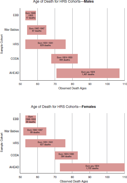
FIGURE 3-1 Observation ages and death counts for the HRS birth cohorts used in the committee’s estimates of the mortality-career earnings gradient. EBB = early baby boom, CODA = children of depression era, AHEAD = birth cohorts included in the original AHEAD survey, which was eventually absorbed into the HRS. Some individuals were dropped from the analysis because of missing values, nonresponse, and similar reasons.
SOURCE: Committee generated from Health and Retirement Study data.
sentation purposes we use the life expectancy at age 50 as a convenient and widely understood summary measure. This requires that future mortality be extrapolated to high ages in future years until each birth cohort has died out. This extrapolation has been carried out on the assumption that all estimated trends continue in the future. These extrapolated trends are quite similar to both Social Security projections and Waldron’s (who uses the Social Security projections), when averaged across gender and income quintile, as will be discussed below. However, because Social Security actuaries assume a future slowing of the historical trend of mortality decline while we assume the historical trend will continue, the committee projections are slightly higher. Projections by gender, however, differ in important ways as will be discussed.
In order to investigate the consequences of mortality inequality for the 1960 birth cohort, we construct a plausible scenario for mortality at ages 50 and above based on our fitted model, on the assumption that the base period trends we observe continue, both in average mortality and, more importantly, in the widening of the differentials by midcareer earnings. This scenario will be referred to as the mortality regime of the 1960 birth cohort, but it is important to keep in mind that it is entirely extrapolated or projected rather than observed.
To be sure, we cannot be sure that the trend in mean mortality will continue, but most forecasters assume that it will. This is approximately true of the projections reported in the Social Security Trustees Reports and in the projections by the U.S. Bureau of the Census. We also cannot be sure that disparities in old-age mortality by midcareer earnings will continue to widen. There is evidence from the cross-sectional studies reviewed above that mortality differences by educational attainment percentile continued to widen between 1990 and 2010 (Meara et al., 2008; Bosworth et al., 2014; Bound et al., 2014), and we are not aware of any evidence that the steepening trend for differences by income has slowed. Nonetheless, there is uncertainty about whether these trends will continue.
UNCERTAINTY OF THE MORTALITY PROJECTIONS
These projections of mortality and its dispersion in relation to midcareer income and by gender are subject to uncertainty from a number of sources. These were discussed above but are summarized here.
- The HRS that we use as our data source for deaths by age and midcareer income covers deaths from 1992 to 2008 for a survey population that started with about 21,000 individuals, a number gradually depleted by death and loss to follow-up and augmented by new recruits above age 50.
- This limits the number of years that each cohort is observed and raises the random component in the number of deaths occurring at a given age, income category, and year. We do observe the mortality experience of 32 birth cohorts, but some are observed for very few years or 1 year. The mortality of each cohort is observed across a different range of ages, with the older cohorts observed at older ages and the younger ones at younger ages.
- There is uncertainty about the appropriate model, including the way to express the trend in mortality.
- Our projections assume that our fitted trend will continue in the future, but the Social Security projections assume that the trend gradually slows.
- All the parameters of the model on which the projections are based are estimated with uncertainty.
- The estimated model itself contains an error term that reflects the inability of the model to fit the data perfectly, which is an additional source of uncertainty in the projected values.
Although the literature contains a number of probabilistic methods for forecasting mortality, they were developed for simpler situations; it would not be appropriate to apply them in this setting. Developing appropriately modified versions of these methods to use here is beyond the scope of the present study. Therefore, although a formal treatment of the uncertainty in our mortality projections is not possible, to address this uncertainty we have constructed a second scenario in which the trend in mean mortality continues but the increase in mortality disparities by income is only half as great for the 1960 cohort as in our baseline scenario. Chapter 4 presents the key results using both the baseline scenario and this scenario with reduced dispersion. While it is also possible that future dispersion will increase more rapidly than our projection, increased dispersion would reinforce the results reported in later chapters, so we focus on the reduced-dispersion scenario, which reflects the opposite possibility, to explore the uncertainty in the results on which the committee’s conclusions depend.
To see how this reduced-dispersion scenario is constructed, consider the top to bottom differential in life expectancy at age 50 for males (difference between the top quintile, Q5, and the bottom quintile, Q1). In the baseline analysis, this differential grows from 5.1 years to 12.7 years between the birth cohorts of 1930 and 1960, or by 7.6 years. In our alternative scenario, it instead grows by 7.6/2 = 3.8 years so that in 1960 the life expectancy at age 50 differential for males is 5.1 + 3.8 = 8.9 years instead of 12.7 years. We cannot give the probability that the actual differential will be greater than or equal to the alternative scenario. It will be possible to see, however, how much difference it would make to our results if the actual widening
of the dispersion in longevity turns out to be only half as large as in our baseline projection.
Much more speculatively, we also calculate for some purposes the projected life expectancy at age 50 for the 1990 birth cohort by income quintile, on the assumptions that the underlying trend in mortality decline remains unchanged from the base period and that the underlying trend in differentials about that trend likewise continues unchanged. This second assumption, about the trend in differentials, is particularly problematic because the differentials are strongly influenced by trends in smoking behavior, including both uptake and quitting—trends that are not expected to continue for long. Thus, these calculations for the 1990 cohort should be taken as illustrative. Nevertheless, the extrapolations for the 1990 birth cohort are useful to provide a sort of upper bound on mortality differentials and policy consequences after midcentury. The committee was particularly interested in the later-born cohorts such as 1960 and 1990 because cohorts such as these will be fully affected by any policy reforms that affect age of eligibility for benefits, such as Social Security retirement, or that interact with age and survivorship in other ways, such as changes in the cost-of-living adjustment.
The results of this estimation and extrapolation are shown in Figure 3-2. In the upper panel for males, for birth years 1930 and 1960, life expectancy at 50 always rises as one moves from lower to higher income quintiles. The difference between life expectancy for the highest and lowest quintiles is 5.1 years for the 1930 cohort and 12.7 for the 1960 cohort (projected).
For females, a similar pattern is observed: higher income quintiles have higher life expectancy at 50, except for the second quintile in 1930. The difference between life expectancy for the highest and lowest quintiles is 3.9 years for the 1930 cohort, slightly smaller than for males, and 13.6 for the 1960 cohort (projected). These quantitative differences are also quite similar to the male differences. We also note that our estimates show a decline of a few years for life expectancy at age 50 for the bottom income quintile and a slight decline for the second lowest income quintile.
As a plausibility check, one can average across gender and quintile to get a cohort life expectancy at age 65, which can be compared to SSA estimates or projections of that same quantity (Bell and Miller, 2005). The agreement is quite good for each birth cohort. Giving the SSA figure first, the comparisons are as follows: for 1930, 17.9 versus 17.5 years; for 1960, 19.6 versus 21.1 years; and for the distantly projected 1990 birth cohort (not shown in the graphs), 21.2 versus 21.8 years. Not surprisingly, the SSA projects that life expectancy will rise more slowly than the projections reported here, which assume that base period trends continue in the future.
If the same calculation is carried out by gender, then anomalies arise. In the committee’s estimates/projections, life expectancy is slightly lower for
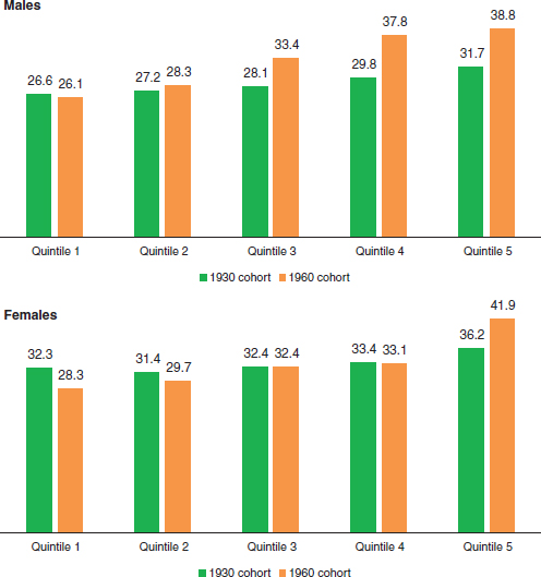
FIGURE 3-2 Estimated and projected life expectancy at age 50 for males and females born in 1930 and 1960, by income quintile.
SOURCE: Committee generated from Health and Retirement Study data.
females than males in the 1960 cohort and considerably lower in the 1990 cohort. Although a narrowing of the male-female life expectancy difference in the future is plausible, it is not plausible that male life expectancy will be higher than female, and this outcome is not consistent with the SSA projections. Thus, one must interpret the gender-specific results with caution. This is frequently the case in the literature. Estimates of mortality differences by income for females are often unstable or present other problems (Waldron,
2007; Bosworth and Burke, 2014). Analysts typically focus on results for males.
Although these summary life expectancy figures are useful and (mostly) intuitive, the probability of survival to specific advanced ages is also revealing. These estimated probabilities, based on the same estimated and projected mortality schedules, are presented in Figure 3-3. One can see, for example, that a top quintile male born in 1930 and surviving to age 50 has a 45 percent chance of living to age 85, whereas a bottom quintile male has only a 27 percent chance. The implications for receipt of retirement and health care benefits are clear. But for the 1960 birth cohort, the corresponding probabilities are 66 percent and 26 percent, rising substantially for the top quintile but holding steady or declining slightly for the bottom quintile male.8
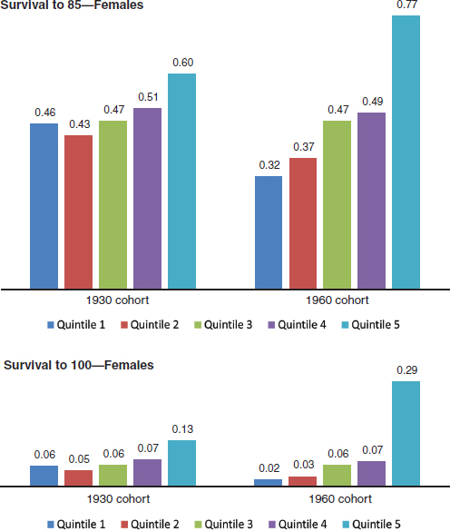
The corresponding percentage probabilities of survival from age 50 to 85 for females are 60 versus 46 percent for the 1930 birth cohort, and 77 versus 32 percent for the 1960 birth cohort. These top quintile females would have more than two times the chance of survival to age 85 as those in the bottom quintile. The projected probabilities for female survival from 50 to 100, shown in the last panel of Figure 3-3, show an implausibly great advantage to the top quintile for the 1960 birth cohort.
This chapter began by noting the increasing dispersion of the income distribution in the United States in recent decades. The committee went on to note the widening of distribution of survival by education group and by income. Although it would be natural to think that the two trends are related, it is important to realize that none of the evidence discussed in this chapter bears on whether or not they are related. The analysis developed first by Waldron (2007), then by Bosworth and Burke (2014) and by this committee in this report, finds a relationship between the income quantile (ranked position) and survival. We find, for example, that survival chances rose more quickly for males in the top 20 percent of the income distribution than for males in the bottom 20 percent. Recent CBO projections also embody an expansion in the mortality gradient by lifetime earnings (see Box 3-1). However, this says nothing about any causal relation between changes in survival and the level of income or its dispersion.
It is true that one possible explanation of the finding about income
________________
8More speculatively, the corresponding probabilities for surviving from age 50 to 100 for the cohort born in 1990 would be 82 versus 24 percent, giving the top quintile male more than triple the chance of a bottom quintile male in the cohort. The contrasts for survival to age 100 are far greater.
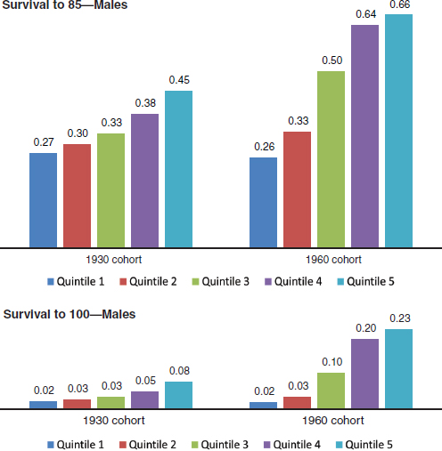
FIGURE 3-3 Proportions of males and females reaching age 50 who survive to ages 85 and 100, by birth cohort and income quintile.
SOURCE: Committee generated from Health and Retirement Study data.
quintiles and survival might be that trends in income distribution mean that those in the bottom quintile are now poorer relative to those at the top than was the case in the past, and therefore their survival has grown relatively worse. None of the studies just mentioned has addressed this important question, which would require different methods and models. Another possible explanation is that inequality itself is bad for health and leads to higher mortality for those at the lower ranks, as has been found in
the famous Whitehall Studies (see, for example, Marmot et al., 1978, 1991; see Box 3-2). A third possibility is that education drives both differences in income and differences in health, and that its relationship to both has grown more steep, leading to a noncausal association of health and income. Doubtless there are other possibilities as well. For our immediate purposes in this report, all that is needed is the association.
BOX 3-1
Congressional Budget Office (CBO) Projections
Official projections from the CBO embody some degree of expansion in the mortality gradient by lifetime earnings quintiles, although both the magnitude and trend (change in slope) of that mortality gradient appear somewhat smaller than the central estimates in this report. The table on the facing page, based on data published by the CBO, shows additional years of life expectancy at age 65 for people who have never received disability benefits. The gap in life expectancy at age 65 between the highest and lowest lifetime earnings quintiles is projected to increase by 2.8 years for males born in 1974 (who turn age 65 in 2039) compared to males born in 1949 (who turn age 65 in 2014). For females, the gap is projected to rise by 2.0 years over the same period.
Direct comparisons of the CBO projections to the estimates in this report are challenging for several reasons, including the differences in birth cohorts (this report focuses on those born in 1930 and 1960, whereas CBO projections show those born in 1949 and 1974); the treatment of those who have qualified for disability insurance (this report includes them, whereas CBO projections exclude them); and the age at which the additional years of life expectancy are measured (this report focuses on age 50 because of the structure of the Future Elderly Model, whereas the CBO examines life expectancy at age 65).
Despite these differences, two features of the CBO projections are worth highlighting. The first is that the CBO, in its official long-term budget projections, assumes that the mortality gradient will continue to widen. However, the second feature is that the CBO appears to assume a more modest degree of steepening over time than does the simple projection of current trends presented here. For example, the committee’s central estimates suggest that the mortality gradient
FUTURE TRENDS IN THE MORTALITY GRADIENT
What will happen in the future to differentials in life expectancy across groups of the U.S. population? The gaps between those at the top of the socioeconomic ladder compared to those at the bottom are likely to persist, but less clear is whether the gaps will widen further or narrow.
The task of predicting the course of mortality is complex, and even more complex is the task of predicting the patterns of differentials. For projecting future trends, patterns of tobacco smoking and obesity and their likely impact on mortality into the future are important. Because both obesity and smoking are distributed unequally across socioeconomic groups in the population, the health and mortality differentials related to them are expected to continue in the future. In this regard, two counteracting influences prevail among young adults who will be of retirement age in the future: smoking has declined but obesity has increased over time (see Fig-
between the lowest and highest quintiles expanded by 3 to 4 months per year, on average, between the 1930 and 1960 birth cohorts. The CBO projections, by contrast, assume that the gradient steepens by 1 to 1.3 months per year, on average, between the 1949 and 1974 birth cohorts. The CBO projections also suggest that the gap increases less for females than males; our projections show the opposite.
Life Expectancy for Nondisabled People at Age 65 by Lifetime Earnings Quintile: 1949 and 1974 Birth Years
| Lifetime Earnings Quintile | 1949 | 1974 | Change in Life Expectancy | |
| Males | ||||
|
Lowest |
22.9 |
24.5 |
1.6 |
|
|
Highest |
26.3 |
30.7 |
4.4 |
|
|
Difference |
3.4 |
6.2 |
2.8 |
|
| Females | ||||
|
Lowest |
26.3 |
28.3 |
2.0 |
|
|
Highest |
27.5 |
31.5 |
4.0 |
|
|
Difference |
1.2 |
3.2 |
2.0 |
|
SOURCE: Based on supplemental data in Congressional Budget Office (2014), see http://cbo.gov/publication/4547 [July 2015].
ures 3-4 and 3-5). Looking at these risk factors in young age is important, because scholars have documented the influence of their presence in young age for age-related risk of dying later in life. There is, for example, evidence indicating that obesity in early adulthood appears to increase mortality at age 50 (Preston et al., 2013).
Because tobacco smoking has continued to decline overall, much attention has centered on the rising obesity trends and whether obesity and its related disease consequences will counteract the possible gains in life expectancy due to declining smoking. A common practice is to classify subjects as underweight, normal, overweight, and obese according to levels of body mass index (BMI). There is repeated evidence, through individual research projects, meta-analyses of a series of studies, and systematic literature reviews, of a nonlinear relationship (J-shape) between BMI and subsequent mortality, wherein researchers find that being overweight in old age may be protective to avoid mortality in case of hospitalizations or injuries (Al Snih
BOX 3-2
Shifts in Income Inequality and the Mortality
Gradient in Other Countries
There has been considerable study of changes in income inequality since the mid-1980s in many countries but relatively little research into the interplay of changing income distributions and changing mortality patterns. Furthermore, changes in mortality gradients by income quantiles (the focus of this report) or other such groupings do not appear to have been investigated and published elsewhere.
With regard to income, the OECD has documented that while real disposable household income grew by an average of 1.7 percent during the two decades prior to the recent global economic crises, the income of the richest 10 percent of households rose faster than that among the poorest 10 percent of households in the great majority of OECD countries (OECD, 2011). At present, the average income of the top 10 percent of the population in OECD countries is approximately 9 times that of the poorest 10 percent. There is large variation among OECD countries, with the top-to-bottom ratio being significantly lower in Nordic and some continental European nations while the ratio reaches or exceeds 14 in the United States, Israel, Mexico, Chile, and Turkey. The OECD calculates that the overall Gini coefficient* increased by about 10 percent between the mid-1980s and the late 2000s, with increases noted in 17 of the 22 OECD nations that have sufficient time series data. A separate analysis of 129 regions in 13 European countries found that the combined absolute gap in average household income between the highest- and lowest-income deciles expanded by 14 percent between 1999 and 2008 (Richardson et al., 2014).
The question whether the dispersion of health and mortality by SES has been widening has not received a great deal of attention in most countries, perhaps because of as-yet insufficient data for establishing a solid connection. In an initial attempt at cross-national comparison, Mackenbach and colleagues (2003) examined national-level longitudinal data on mortality by occupational class and educational attainment from Denmark, Finland, Sweden, Norway, Britain (England
et al., 2007). Overall, however, underweight and especially obesity in old age confer heightened risks of dying (Flegal et al., 2013; Masters et al., 2013; Winter et al., 2014). Obesity-related conditions include heart disease, Type 2 diabetes, and certain cancers, which are some of the leading causes of “preventable” deaths.
As mentioned before, the influence of smoking and obesity on differentials in mortality depends on how unequally they are distributed in the population. Although tobacco smoking has declined overall, the difference in prevalence of smoking by income level (measured relative to the poverty line) has remained roughly the same over the past 20 years (see Figure 3-6). In 1990, 40 percent of males aged 18 and older in the low end of the
and Wales), and from Turin in Italy. Looking at the time periods 1981-1985 and 1991-1995, they concluded that relative inequalities in overall mortality increased in all countries, often because mortality from cardiovascular disease declined relatively faster among higher socioeconomic groups. More recent and expanded comparative work has documented persistent differences in health status among socioeconomic groups in 18 European countries (University Medical Centre Rotterdam, 2007).
Researchers in the United Kingdom have had a longstanding interest in the relationship between SES and health. The well-known Whitehall Studies I and II (begun in 1967 and 1985, respectively) have been linchpins in the development of research in this area and have shown a clear and powerful association between health and social class. Subsequent studies and reports have demonstrated a widening mortality gap between social classes from the 1950s through the mid-1990s and persistent gaps in life expectancy through the mid-2000s (United Kingdom House of Commons, 2009; Marmot et al., 2010; Dorling, 2013).
Unlike the situation in Britain, there does not appear to be a clear relationship between increasing income inequality and changing health in Canada. Recent analyses (Anderson and McIvor, 2013; Conference Board of Canada, 2014) have documented rising income inequality during 1990-2010; by 2010 the top income quintile received 39 percent of total national income compared with 7 percent for the lowest quintile. The Conference Board of Canada analysis concluded that health was seemingly unaffected by the rise in income inequality. And a report from the Public Health Agency of Canada (2011) asserts that differences in health between the highest- and lowest-income groups generally have been lessening over time, albeit with exceptions (e.g., the low-high income-group difference in diabetes mortality increased 40 percent during the first decade of the 21st century).
_________________
*The Gini coefficient is a measure of statistical dispersion that represents the degree of inequality in the income distribution of a population. The coefficient varies between 0 (complete equality) and 1 (complete inequality).
income distribution (below 100% of the poverty line) were smokers, compared to 22 percent of their counterparts in the high end of the distribution (above 400% of the poverty line). By 2010, the comparable figures were 33 percent and 13 percent, respectively. The gap in smoking between poor and rich hovered around 15 to 20 percentage points over the 30-year period. Figure 3-6 shows a similar trend for females, except that the poor-rich gap widened slightly over time.
For obesity, although the pattern has been of rising prevalence for individuals at all levels of income over time, the difference in prevalence between the low- and high-end income groups over the years 1990 to 2010 has actually narrowed (see Figure 3-7). By 2010, among the U.S. population
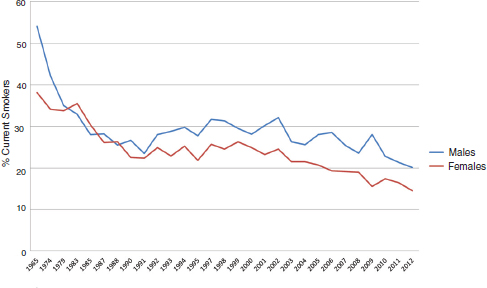
FIGURE 3-4 Smoking among U.S. adults aged 18-24, by gender, 1965-2012. Estimates are for current cigarette smoking.
SOURCE: Based on data from the National Health Interview Survey, see http://www.cdc.gov/nchs/hus/healthrisk.htm [July 2015].
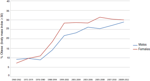
FIGURE 3-5 Obesity among U.S. adults aged 20-34, by gender, 1960-2012. Body mass index (BMI) equals weight in kilograms divided by height in meters squared. Obesity equals BMI greater than or equal to 30.
SOURCE: Based on data from the National Health Interview Survey, see http://www.cdc.gov/nchs/hus/healthrisk.htm [July 2015].
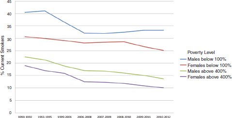
FIGURE 3-6 Smoking among adults aged 18 years and older, by gender and poverty level, in the United States, 1990-2012. Estimates are for current cigarette smoking, age-adjusted to the year 2000 standard population using five age groups: 18-24 years, 25-34 years, 35-44 years, 45-64 years, and 65 years and older. Poverty-level data are percentages of the estimated poverty thresholds set by the U.S. Census Bureau and based on family income and family size and composition.
SOURCE: Based on data from the National Health Interview Survey, see http://www.cdc.gov/nchs/hus/healthrisk.htm [July 2015].
aged 20 and older who were in the low end of income, 37 percent were obese, compared to 31 percent of their high-income counterparts. Interestingly, the narrowing gap in recent years between the two groups is due to a relatively higher rise in obesity among the rich compared to the poor.
Thus the expectation is that the gains in life expectancy that previous cohorts enjoyed could be somewhat curtailed by prevailing smoking and obesity patterns. One study (Preston et al., 2014) makes projections for 2010 to 2040 using data for the cohorts that were age 25 in 1988 to 2006. As expected, the prediction is that changes in smoking and obesity will have large counteracting effects on the mortality of older U.S. adults. For males, the combined effect will be 0.83 years of gain in life expectancy by 2040, but for females the gain will be much smaller, 0.09 years by 2040.
What is harder to predict is the impact of medical advances and other relevant changes on future health outcomes and life expectancy. It is certainly possible that with advances in oncology and other fields, life expectancy at older ages may rise substantially in the future.
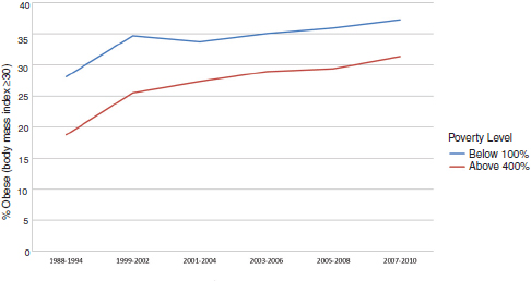
FIGURE 3-7 Obesity among adults aged 20 years and older, by poverty level, in the United States, 1988-2010. Body mass index (BMI) equals weight in kilograms divided by height in meters squared. Obesity equals BMI greater than or equal to 30. Percentage of poverty level is calculated by dividing family income by the U.S. Department of Health and Human Services’ poverty guideline specific to family size, appropriate year, and state. Percentages are of the estimated poverty threshold.
SOURCE: Based on data from the National Health Interview Survey, see http://www.cdc.gov/nchs/hus/healthrisk.htm [July 2015].
Even if innovation increases life expectancy in the future, it may widen inequality in life expectancy. Access to innovative health technology (e.g., new treatment for a major chronic disease) has been historically unequal because of the nature of new discoveries, which tend to be relatively costly to implement at first. Thus the groups in the high end of the income distribution are likely to benefit from new medical technology first, producing and exacerbating health disparities. A similar conclusion is reached by researchers who document a wider gap in disparities by education groups when new medical technologies that require sophistication are introduced (Goldman and Lakdawalla, 2005). Because new technologies are expected to continue to propagate and be adopted differently by groups within the population, significant health disparities from this source are expected to prevail in the foreseeable future (Rogers et al., 2013).
Unequal ability to manage diseases by ill persons in the high end of the income distribution compared to those at the lower end has been proposed as a persisting source of the health gradient. There is evidence that the health gradient across educational groups of the U.S. population is in part
due to disparities in adherence to treatment. Goldman and Smith (2002) use diabetes and HIV as cases to illustrate this contribution to the health gradient.
Another important influence on future patterns of mortality differentials will be the impact of ongoing health care reforms in the United States. By providing increased access to health care to groups that lacked access previously, will these reforms produce narrowing gaps in risks of dying across socioeconomic groups? Research conducted to assess the consequences of not having health insurance concludes that the benefits of insurance are significant for the population in good health. In addition, a report from the Institute of Medicine (2009) found evidence of a secondary effect operating through the supply of health care services in the community. If communities are heavily uninsured, then the supply of services tends to be relatively low or of lower quality, thus affecting negatively even the health care of the insured groups living in the same community. If these arguments are applied to an increase in health insurance coverage due to health care reforms, then the past evidence would suggest that increased access to health care could result in higher use of preventive services, reducing premature death. Similarly, earlier detection of cancers and diminished risk of cardiovascular diseases, stroke, and injuries would be expected. However, evidence on the effects of recent reforms is not yet available.
Thus, uncertainty remains about whether mortality disparities will widen or narrow in the future. The committee’s analysis does not assess the various causes of mortality and its disparities; it is instead a reduced-form extrapolation of previous trends. In the absence of clear evidence from a cause-based analysis, however, we view the trend extrapolation as an acceptable approach to a central estimate for the future.
ADDITIONAL CAVEATS TO THE MORTALITY ANALYSIS IN THIS REPORT
The discussion in this chapter has highlighted several caveats that apply to the chapter analysis and by extension to other parts of the report. By way of summary, the committee notes that although there is broad agreement among researchers that the dispersion of mortality by SES has widened in the United States in recent decades, there is uncertainty about the speed, extent, and differences by gender. We have used the HRS as our primary dataset for analysis of mortality as well as for other purposes, and both its sample size and the range of years it covers are smaller than one would like.
To be relevant for current policy choices, the committee has simulated outcomes for the generation born in 1960, but the HRS does not contain mortality data for this generation because it does not reach the age of 50 (at which primary eligibility for the HRS begins) until 2010, and the latest
HRS administration used for this report was in 2008. Therefore, we had to simulate or project the mortality of this generation. The committee did have data for at least a few years for generations born up to 1953, but we had to extrapolate for at least 7 years on the assumption that earlier observed trends continue. Furthermore, as discussed earlier, the analysis observes the mortality of more recent generations only when they are in their 50s, whereas it observes the mortality of earlier born generations at older ages such as in their 70s. Fortunately, Waldron (2007, 2013), using the larger Social Security dataset, confirms that differentials are widening even when all generations are observed at the same younger ages.
We have avoided any causal interpretation of the widening trends we observe because our calculations do not require one. The simple association is sufficient to calculate the consequences for the progressivity of various public programs. Although it would be useful to know whether the widening distribution in earnings is a cause of the widening distribution of mortality and life expectancy, the committee’s analysis does not address this issue. There are many other points that similarly are not addressed—for example, the relative roles, if any, of education, smoking, and obesity. These topics deserve study in their own right.
The measurement of lifetime earnings used by the committee follows other recent literature, but it is a compromise forced on us by the history of Social Security coverage and benefits. We, like others, have used the average of earnings during years when earnings were positive, for a span of 10 years near typically peak earnings. The whole earnings history cannot be used because many workers in earlier cohorts joined Social Security well after they began working, so Social Security earnings histories miss a segment of their earlier earnings.
In light of its deliberations on the data and the literature, the committee believes that policy makers and researchers alike should pay more attention to the distribution of life expectancy—and not just to changes in average life expectancy—because it appears that something of importance is occurring that has received too little attention. We acknowledge, however, that this report has significant limitations with respect to the available data and the necessary analytical assumptions described in this chapter. The committee therefore hopes that the report will spur further research and discussion of trends in life expectancy inequality, much as the literature on income inequality has expanded over the past two decades.


