Assessing the Use of Agent-Based Models for Tobacco Regulation (2015)

Appendix B

Agent-Based Models for Policy Analysis

Lawrence Blume¹

WHAT IS AN AGENT-BASED MODEL?

An agent-based model (ABM) is a computational simulation model of a many-agent system that captures the behaviors of the system’s autonomous agents and their interactions with each other. An ABM is a computational instantiation of a complex adaptive system (CAS). A CAS is a dynamic model that represents individual agents and their collective behavior.² In social science applications, agents are usually people. CASs, however, have applications in many different systems, in which agency has many different interpretations. Generally speaking, an agent is a persistent entity that is described by states and behaviors, which are consequences of the agent’s state. The agent’s state is modified by its interactions with other agents. The agent population is usually not modeled as a “gas” of randomly interacting particles.³ Instead there will typically be some structure to agents’ interactions: The set of others with whom any agent can interact is circumscribed. This structure is usually described by a social network; agents interact only with their neighbors.

______________

¹Cornell University, IHS Vienna, and Santa Fe Institute.

²The study of CASs, both theoretically and through computer simulations, was central to the research program of the Santa Fe Institute in the 1980s and 1990s and was stimulated, in particular, by John Holland’s work on genetic algorithms and classifier systems. His 1975 book (Holland, 1975) was certainly influential at SFI.

³In models describing social phenomena at higher levels of aggregation, the “gas” assumption is common. See the discussion of the SIS model below.

The states of individual agents may behave erratically. Nonetheless, some aggregates of agent behavior may exhibit stable regularities. These regularities are referred to as emergent behaviors. The equations describing a CAS are descriptions of behavioral rules for the autonomous agents and descriptions of how they interact. The driving equations of the system are typically at the level of the individual agent, and describe action at temporal scales appropriate to the agent. An emergent property is a regularity in the output of the CAS that appears robustly on a temporal or spatial scale different from those of the driving equations. Emergent properties, the behaviors of the whole, are the objects of interest in a CAS.

An ABM is a computer program that implements a CAS by simulating its behavior. The CAS describes a probability distribution on outcomes for every vector of inputs x and equation parameters p, and the ABM simulates the probability distribution. Each run of the program yields a random draw from the CAS’s outcome distribution, and so the empirical distribution of many draws approximates the CAS’s outcome distribution.

At the risk of being either too mathematical or too redundant, I will finish this section by recasting a familiar epidemiologic model as a CAS and compare the CAS representation with more familiar representations. The annex contains a more formal mathematical description of CASs.

The SIS model is a textbook model of the spread of a disease. At any moment, the individuals are of two types, or states: susceptible (S) and infected (I). The infected individuals can transmit the disease to the susceptibles. The numbers of people of each type at time t in a fixed population of size N are denoted S(t) and I(t), respectively. The point of the model is to track the path of the population through these states over time. A continuous-time SIS model might presume that the population contains a continuum of agents of mass 1. The population aggregates evolve according to the following differential equation system:

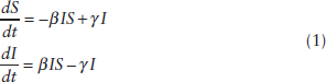
The SIS model is an aggregate-level model of an epidemic with the happy feature that no one dies from the disease. It could also serve as a model of the spread of a rumor (although the well-known SIR epidemiological model would be a better metaphor). The parameter b is the transmission rate, and g is the recovery rate. A solution to the deterministic model is a function that describes the evolution of S(t) and, by implication, I(t) through time. The SIS model is a “gas model” in that key to its deriva-

tion is the assumption that the population contains many individuals and in any unit of time each individual is equally likely to interact with any other individual.

Equation system 1 is meant to model the aggregate behavior of a gas model of individuals—individuals bump into each other randomly. If a susceptible individual and an infected individual collide, the susceptible individual becomes infected with probability b. Furthermore, an infected individual becomes cured with probability g. The hope is that the differential equations provide a good approximation of a large-population version of the gas model.

The aggregate behavior of the stochastic gas model is often described as a birth–death process. This is a Markov process on the number i of infectives. The time interval h of a single period is so small that at most a single transition takes place in each time interval. That is, if I(t) = i in period t, then I(t + 1) can have only the values i + 1 (a “birth,” or infection), i, or i 1 (a “death,” or recovery). The probabilities of births and deaths when I(t) = i are denoted by p_i and q_i, respectively, and they have the values

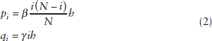
The equations (2) describe a stochastic process, a joint probability distribution of the collection of random variables {S(t)}^∞_t=1. A single draw from that distribution is a sample path of the number of susceptibles. A textbook theorem says that the solution to the differential equation approximates the path of the stochastic process uniformly well over any finite time horizon if h is small enough and N large enough. That justifies the use of the differential equation, but only up to a degree, because the asymptotic behavior of the differential equation does not in general approximate the asymptotic behavior of the stochastic process.

A CAS model of the same process describes the circumstance of each individual in the population. Thus, a state, or configuration, of the CAS is a vector of length N in which the nth component describes the state of individual n, S (susceptible) or I (infected). The CAS has a list of rules that describe how each individual responds to interactions with others and to exogenous random events. For the illustrative SIS CAS, all individuals have the same rule, which is described in Figure B-1. On every date, one of three things can happen to a susceptible individual: they can be matched with a healthy individual, event h; with an infected individual, event i; or with no one, event 0. The same three events can happen to an infected individual,

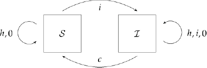
FIGURE B-1 Individual state transitions.

and in addition he or she can be cured, event c. The boxes represent their possible states, susceptible, S, and infected, I. The arcs represent the transitions that each event causes: For instance, if a susceptible individual is matched to another susceptible individual, their state remains unchanged.

To complete the description of the CAS, the interaction process and the exogenous event process must be described. There are N(N – 1)/2 possible unordered pairs that can form, and there are I possible cures. There is also the possibility that nothing will happen. Thus, in any state of the system that has I infecteds, there are N(N – 1)/2 + I + 1 possible events. In each period, taken to be of very short duration h, one and only one of those events will be drawn. Suppose that the probability that any particular pair will form is βh/N, that a cure for a particular infected individual has probability γh/N, and that nothing will happen with the complementary probability. Because h is small, the pair formation and recovery numbers and 1 minus their sum are nonnegative, so they describe a probability distribution on the set that consists of the pairing events, the recovery events, and the event that nothing happens. Then the stochastic process of the number of susceptibles in the CAS is exactly the birth–death process described by equation 2.

Emergent properties of the CAS have to do with the behavior of aggregates, such as the number of susceptibles. This CAS is a Markov process that has a single absorbing state in which no one is infected; that is, the disease has died out. The distribution of the extinction time, which describes the behavior of the amount of time it takes to reach that state, is another emergent property.

An ABM would implement this CAS in a computer program by iterating the following scheme: Starting with an initial configuration, use a random-number generator to choose a feasible event according to the probabilities described above. If the event is a match, every individual other than the matched pair receives input 0, and each individual in the pair receives the state of their partner. If the event is a cure, the input to the cured individual is the event c, and all other individuals receive a 0. The state of

each individual is then updated according to the rule of Figure B-1, and the result is a new configuration.

If we are interested only in the aggregates, there is no advantage to constructing the CAS; there are easier ways to simulate the SIS process than by building an ABM. But now make the model more complex. Suppose that individuals are differently susceptible to the disease; that is, b is now individual-specific. Aggregate behavior can still be modeled with a Markov process, in this case a multitype birth–death process, with one type for each level of susceptibility. But such processes are more difficult to analyze, and if every individual has a different susceptibility to the disease, the resulting multitype birth–death process in a population of size N is essentially the CAS. Even more interesting is to suppose that the population has a spatial structure and individuals either meet only neighbors or meet neighbors more frequently than others. Now one needs the CAS to keep track of things. The network becomes a parameter of the CAS, and with an ABM one can ask how, for given b and g (and h), the shape of the network matters. The CAS can be still more complex. A given set of individuals could be designated as “health care workers” who have higher probabilities of interacting with infected individuals, and so on.

The aggregate behavior of the simple CAS can be usefully approximated for large N and small h over finite time horizons by the differential equation system 1, and a similar system approximates the multitype version when there are many more people than types. If the social structure of the networked model is something regular, like a lattice, it is possible to approximate the system with a partial differential equation if the large-N question is posed the right way. Such approximations are known as mean-field approximations. For more realistic social networks, it is not clear how to pose the large-N question.

CASs force a bottom-up approach to modeling systems. The modeling exercise requires a description of the set of individuals, their behavioral rules, and a description of how they interact. That is in contrast with top-down descriptions, such as equation system 1. One virtue of bottom-up modeling is that the derived aggregate system is guaranteed to be consistent with some actual social process. A further advantage, as this example illustrates, is that bottom-up models support a degree of complexity that is not available in aggregate models. In particular, heterogeneity in agent behaviors and heterogeneity in the variety of interactions available to agents in different roles need more complex descriptions than top-down models can provide.

THE USES OF AGENT-BASED MODELS

ABMs, like other mathematical models, serve three purposes: demonstration, description, and prediction. In the 1980s and 1990s, the primary

use of ABMs was to “show off” the kinds of emergent behavior that a system could produce. A good example of that is Schelling’s segregation model (Schelling, 1971). It is described by a small number of parameters whose purpose is to show that an emergent property—completely segregated neighborhoods—is a consequence of individual decision rules that exhibit a very small “taste” for similar neighbors. Schelling describes his 1971 paper as “an abstract study of the interactive dynamics of discriminatory individual choice” (p. 143). Many demonstrations are just theoretical exercises in models that cannot (yet) be accessed analytically. I put yet in parentheses because analytic technique does advance. Schelling’s model could not have been addressed with tools that were available in the late 1960s, but developments in so-called particle systems have made the formal analysis of his model straightforward.⁴ Generally speaking, models like Schelling’s generate useful theoretical conjectures that can be explored with a variety of methods.

The Hoffer et al. (2009) model of a local heroin street market in Denver is a more sophisticated use of an ABM. The authors use ethnographic data collected by the principal author, an anthropologist, to calibrate an ABM. The ethnographic research concentrated on individual behaviors and interactions of the different actors in the market. The authors make it clear that “the model described in this manuscript is not intended as a forecasting tool” (p. 273). The purpose of the ABM was to uncover emergent properties of market behavior that could not be observed at the scale of ethnographic research. As far as I can tell (the paper is not entirely clear on its methods), the model is calibrated to ethnographic data. Simulations are then run at a market scale to observe the emergent properties of the market system. The model is complex. It contains six types of agents, each with its own rules of interaction and repertoire of behaviors: customers, brokers, sellers, private dealers, police, and homeless people. The customer agent in particular has complex demand behavior that reflects known facts about heroin use. The large-scale properties of the heroin market are likely to be measurable only with great difficulty, so using a simulation model that is based on more easily observed individual behavior patterns is a clever idea. One’s confidence in the model’s macro-level predictions depends on one’s confidence in the internal validity of the model, that is, how well it matches the ethnographic data and how well the ethnographic data capture the fine details of the agent interactions on which the model most sensitively depends. Ideal research design would require dialogue between ethnographers and modelers about the research strategy and the modeling activity. That was impossible in this case because the modeling took place

_____________________

⁴See Young (2001).

nearly 15 years after the ethnographic research was carried out.⁵ The ABM generated some interesting hypotheses about the large-scale behavior of the street market. One interesting experiment is the simulation of a one-night police crackdown. The model showed a short-term effect on all market agents and a sharp decline in transactions. But sales through other channels, particularly private dealers, led to a rebound in transaction volume, and the simulation showed that the police crackdowns had no long-term effect. This detailed model, tightly coupled to a particular market, suggests interesting hypotheses about the effects of policing strategies. The authors are circumspect about the generalizability of their analysis, however, noting both data lapses and peculiarities of the particular market that they studied.

A more ambitious research program is reported in Eubank et al. (2004) and Toroczkai and Eubank (2005). The subtitle of the work by Toroczkai and Eubank (2005) describes a policy problem: “How to halt a smallpox epidemic.” An ABM of the spread of smallpox through a city is calibrated on pre-existing data, and then the effects of several different vaccination regimens are simulated. No U.S. city has experienced a smallpox epidemic in recent times, so the data on which the model is calibrated come from a world in which smallpox is absent. The model is then used to simulate counterfactual worlds in which smallpox is spreading (a consequence, presumably, of some biowarfare or terrorist event) and different vaccination strategies are deployed. The model has three components: an urban transportation component, a detailed epidemiological model of smallpox transmission, and a model of disease detection.

The urban transportation simulation model is used to simulate the daily movements of individuals across locations. From this, contacts between individuals are captured and a contact graph is constructed. The urban transportation component is quite complex. It is an ABM of urban transportation designed to describe Portland, Oregon. A synthetic population is constructed whose distribution of demographic and other characteristics matches that observed in Portland census data. Survey data are used to construct activity patterns for households. Activity location is estimated from land-use and transportation-cost data. From this, routes and travel times for each individual are forecast. From this modeling exercise it can be determined that individuals i and j are in the same location at such-and-such a time. In this manner, a representative contact graph is constructed—who met with whom on a representative day.

The model of smallpox spread from an initial population of infectives is deployed on the contact graph. This too is quite complex, displaying a great deal of biological specificity that I will not describe. The third com-

_____________________

⁵This comment is not meant as a criticism of an exploratory methodology paper whose purpose was to demonstrate the utility of modeling tools in the ethnographic community.

ponent links actual (simulated) disease spread with the observations that drive these policies.

Four modeling exercises are carried out: A baseline simulation with no treatment, mass vaccination of 100 percent of the population over four days, targeted vaccination and quarantine with “unlimited resources,” and a limited resource targeted vaccination and quarantine policy. The conclusion is that targeted response can be effective if detection is sufficiently fast. Mass vaccination is not necessary.

The qualitative result, that policies alternative to mass vaccination could conceivably work, is perhaps interesting. The quantitative results of the simulation exercise, and the conclusion that a targeted vaccination scheme would be as effective as mass vaccination in the Portland of today, are not reliable due to assumptions implicit in the way the model is constructed. For example, we might imagine that knowledge of a spread of smallpox cases would cause people to alter their daily routines. The “representative contact graph” derived from the urban transportation model calibrated to data from a smallpox-free Portland might look very different from a graph of social contacts in a Portland where smallpox is rampant. I will argue below that ABMs that are complex enough to demonstrate or describe possible policy effects in interesting environments will almost certainly fail to measure causal effects to the satisfaction of at least some social science communities.

CAUSATION AND STRUCTURAL MODELS

Empiricists today nearly universally accept Hume’s idea that necessary—that is, causal—connections cannot themselves be perceived, that only recurring associations can be observed, and that the fundamental problem of empirical science is to distinguish the causal relationships among all the associations that appear in data. Hume offered two definitions of cause, the second of which has been influential in statistics and the sciences: “We may define a cause to be an object followed by another, . . . where, if the first object had not been, the second never had existed.”⁶ The contemporary instantiations of that idea are counterfactual theories of causation.⁷ Those theories consider a number of possible or hypothetical worlds. In a world in which X = x and Y = y, the claim that X causes Y is considered by examining nearby worlds in which X ≠ x. The claim is established if, in worlds that differ only in the assignment of the X value, Y ≠ y.

__________________

⁶Hume (1777) sec. 7, part 2. Italics in the original.

⁷Proponents of this view include the late David Lewis (1973) and Nancy Cartwright (1979, 1989). A recent expression of this theory is Judea Pearl’s book (2009). A formal description of some of Pearl’s ideas has been developed in Halpern and Pearl (2005a,b).

That loose description of possible-worlds semantics is made rigorous through the use of structural models. For our purposes, a structural model contains a system of equations that describes a set of hypotheticals or possible worlds. The possible worlds are ones that satisfy some rules that are meant to be descriptive of the phenomena that the model addresses. For example, in a social-science model, these would include assumptions about how individuals interact and rules for their behavior. The SIS CAS is a structural model. Its equations describe how individuals meet and transmit a disease and how they are cured—a combination of social and biologic rules. The equation system of a structural model contains functional forms, variables, and parameters. Each specification of parameters defines a structure, a possible world, and a specific set of relationships among the variables. The variables themselves are partitioned into exogenous and endogenous variables: those determined outside the model and those determined within the model.⁸

The set of possible worlds to consider in adjudicating causal claims is described by the model. Hume’s counterfactual definition of causation leads to a deep point about the nature of causal claims:

Without a theory, there can be no causal claims. And if all causal claims are relative to particular theories, we are freed from the obligation to find the one true model, the root causes, and can instead look for models that

_____________________

⁸Equation systems are somewhat arbitrary. An equation y = ax + u can be rewritten as x = βy + υ where β = 1/α and υ = u/β. But the causal arrow in the first equation points in the opposite direction from the arrow in the second. The geneticist Sewall Wright (1921, 1925) and later the economist Jan Tinbergen (1968) supplemented their equation systems with a diagram, later called a “path diagram,” a graph with nodes that represented variables and directed edges pointing in the direction of causal effects. In his work on causality, Pearl (2009) takes the diagram to be the primitive causal model. Another approach to the problem was taken by the researchers at the Cowles Commission for Research in Economics for the case of linear-equation systems (Hood and Koopmans, 1953). They used transformations of equation systems to determine classes of equivalent systems, all members of which expressed the same causal relationships.

are consistent with the data and address just those questions that we want to ask.

Policy analysis is concerned with three kinds of questions. The first kind asks for the effect of policy X on outcome Y in a given environment E; this is the classic treatment-effects problem. The second is to infer from the effect of X on Y in E the effect of X on Y in a different environment E′. The third is to infer from the effect of X on Y in E the effect of a different policy X′ on outcome Y (or even a different outcome Y′) in a different environment E′. The last two questions, requiring extrapolation, are fundamentally different from the first in that they require us to use the laws uncovered in the analysis of X and Y in environment E to make predictions about a different environment and perhaps a different policy. For example, in the SIS CAS model, the parameter β is the product of two parameters: β₁, the probability that two individuals meet, and β₂, the probability that the disease is transmitted at a meeting. Suppose that β₁ is a policy variable that can be controlled by, say, a policy of identifying and isolating infected individuals. By estimating β₂ and g, we can estimate the distribution of the time to extinction of the disease for a given policy β₁. Suppose now that we expect a new variant of the infective agent to sweep through the population with a lower recovery rate γ ′. With knowledge of the structural parameter β₂ learned in the initial environment, we can forecast the extinction-time distribution for other policies β′₂ in the new environment γ ′.

Unlike the treatment-effects question, these questions require uncovering the parameters of the model, that is, uncovering behavioral laws that remain valid in environments other than E, and in particular environment E′, that we want to study. The more “fundamental” or “deeper” the behavior relationships in the model, the larger its domain of applicability, that is, the richer the sets of environments and policies that it can address. For the purposes of policy analysis, the analyst considers a set of possible policies and environments. The model is required to be sufficiently “fundamental” that its relationships are valid for all policies and environments under consideration. I will refer to that as Marschak’s stability requirement because Jacob Marschak (1974) was the first to pose it explicitly in a discussion of what makes a good structural model. In contemporary macroeconomics, the phrase Lucas critique, in honor of Robert Lucas (1976), is often applied to claims that the behavioral equations of some models are not invariant under alternative macroeconomic policies, that is, that they fail Marschak’s stability requirement.

ABMs are structural models. They describe agents’ rules for processing information and making choices and for how agents interact. They are useful for demonstrating potential policy outcomes; in particular, they may alert us to emergent consequences of policies that those who design policy, thinking at the behavioral level, may miss. They also allow us to test the

reasonableness—the plausibility—of our behavioral assumptions. Nonetheless, they have only limited uses in the statistical analysis of causation and for the extrapolative exercise required for counterfactual policy analysis.⁹

STATISTICAL ISSUES RELATED TO AGENT-BASED MODELS

The purpose of ABMs is to simulate the microbehavior and macrobehavior of CASs, particularly those whose descriptions are too complex to be studied with analytic methods. The necessary complexity of these models makes them large: the smallpox-epidemic ABM (Eubank et al., 2004; Toroczkai and Eubank, 2005), for instance, has over 30 parameters. Those parameters describe different parts of the model, including the course of the disease in a given host (for several variants of the disease), the transmission model (including shedding of an individual’s viral load to the environment and uptake by an individual from the environment), the effects of vaccination, and the traffic-simulation tool, which is used to provide a fine-grained description of how the population mixes over a period of weeks.¹⁰

Using this model to simulate the effects of different vaccination policies requires knowledge of all the parameters. ABM practitioners use such terms as validation and calibration (inconsistently) to describe methods for choosing parameter values. Tesfatsion (2015) describes three approaches to validation. Input validation attempts to use parameter values that come from external knowledge of microbehavior, such as information about the course of smallpox in a single individual; this is the principal validation tool for the disease parts of the smallpox ABM because we have no episodes of smallpox epidemics in recent U.S. history. Descriptive output validation matches computationally generated output with preexisting data on the process being modeled; for example, one might fit the SIS ABM to data on chickenpox by choosing parameter values to match data on the time path of chickenpox incidence in a given location and year. Finally, predictive output validation matches model outputs to subsequently observed datasets. It

_____________________

⁹Approaches to causal inference vary across the disciplines in the social sciences. The approaches can be divided into two groups. One group believes causal claims cannot be established without some kind of counterfactual analysis. A more permissive group is comfortable with causal inference from observational data without an implicit or explicit experiment in the background. I stand with the first group. This group itself is divided into those who require a well-motivated model to make causal inferences and those who are willing to infer causation from randomized trials or so-called natural experiments. Although both groups have a lot to argue about, they would certainly agree that is hard to imagine the natural experiment that would identify the effects of alternative vaccination strategies on a smallpox outbreak in a moderate-sized American city. Put more technically, the stable unit treatment value assumption is unlikely to be met for treatment effects one would want to analyze with an ABM.

¹⁰More recent information about subsequent development of the epidemic simulation modeling tool can be found at http://www.lanl.gov/programs/nisac/episims.shtml.

seems that, generally speaking, two general procedures are used to choose parameter values: choosing them from preexisting studies and choosing them to match statistics of actual and simulated datasets.

The smallpox ABM illustrates a problem that I believe is common in computational models that have many parameters and which makes use of “input validation,” that is, choosing parameter values on the basis of out-of-simulation considerations. One would not expect many of the parameters affecting people’s travel behavior and contacts to be invariant to the onset of a smallpox outbreak. The failure of parameter invariance to counterfactual initial conditions under consideration, and through a typical run of the model, means that the behavioral relations driving the model are not stable under the counterfactual scenarios that we want the model to examine, so the ABM fails the Marschak criterion. Input validation alone is reasonable for demonstration purposes but not for proof of concept.¹¹ The problem of parameter stability is often discussed in the context of estimating structural models, but it is even more critical for models that have externally validated, “input-validated” parameters.

Before turning to issues of ABM parameter estimation, I want to mention a fundamental question about the choice of parameter values for policy evaluation: What does it mean to have good parameter estimates? The purpose of ABMs is to study emergent behavior of a system. An empirically successful ABM will get the microbehaviors right, so the agents in the model approximate in some useful way the behaviors of agents in the world. The ABM will also accurately describe the macrobehaviors, the emergent properties. That is an enormous undertaking for any large-scale computational model. A similar problem arises in the currently popular Dynamic Stochastic General Equilibrium (DSGE) computational macroeconomic models. Instead of having many agents, these models attempt to capture individual behaviors with a small number of representative types. Their goal is nonetheless to capture emergent behavior, in this case that of macroeconomic time-series of interest, such as gross domestic product, inflation, and unemployment. DSGE practitioners use the same calibration and validation techniques that are used in ABMs. Early DSGE practitioners uncovered a dilemma: If they calibrated the parameters of the representative agents to values found to be reasonable in microeconomic studies, they would incorrectly forecast the macroeconomic data. On the other hand, calibrating to the macroeconomic data required microeconomically implau-

_____________________

¹¹I chose this model because the subject matter is a typical ABM application and exhibits the complexity that one often sees in ABMs and because publication in Nature and evidence of successful grant applications suggest that it is not regarded as a horrible exemplar of an ABM put to the purpose of counterfactual analysis. I did not cherry-pick the model, and I do not believe it to be different in kind from many other ABMs that have been studied.

sible parameter values. Validation poses a tension between different ways of “getting it right.” In principle, one would get right both the microbehavior and the macro-level behavior, but this may be impossible. If so, the modeler has to make a choice. DSGE macroeconomists chose to sacrifice behavioral realism to make the macro-level behavior most closely match the data.¹² But doing so makes the whole exercise nothing more than elaborate curve-fitting. Although ABMs may be satisfactory for demonstration purposes, this problem makes them bad policy analysis tools, for two reasons: First, many things that we might wish to calculate, such as the agents’ economic welfare or utility, depend on the microparameters, and calculations with the wrong microparameters are likely not to remain stable in counterfactual scenarios—Marschak’s stability requirement again.

IDENTIFICATION

It would seem, putting aside the calibration and validation problems raised in the preceding paragraph, that ABMs are useful for predicting the effects of novel policies in complex environments. Ironically, however, the virtues of ABMs—their expressiveness, their ability to capture fine-grained details of the workings of the system under study, and their ability to display emergent properties of the system—make them difficult to use for policy analysis.

ABMs describe a recursive system. At the end of each period, the system has a current state and a current behavior for each individual. Those determine, perhaps probabilistically, the next period’s state. The new state and each individual’s behavior determine a new behavior, and so on. The annex contains a formal description of the system. The model is described by an initial (distribution of) state(s) and an initial (distribution of) behavior(s) for each individual. Statisticians observe a run of the system, or perhaps some particular statistics, functions of the history of states and behaviors. We refer to what they see as an “observable.” The model generates a distribution of observables.¹³

The value of a structural model is in its extrapolative abilities. Suppose that it is known with high confidence, after observing data from one

_____________________

¹²For instance, when the capital/output ratio in an economy increases, the return to capital decreases. The share of capital in national output increases or decreases depending on the product of the two terms. Whether that share increases or decreases depends on whether a parameter of production processes, the elasticity of substitution, is above or below 1. This parameter measures how easily capital can be substituted for labor in production. Microeconomic studies typically find the number to be less than 0.75, but matching the macroeconomic data requires it to exceed 1. DSGE modelers choose descriptive output validation over input validation; this has implications for the predicted distribution of income.

¹³The derivation is described formally in the annex to this appendix.

environment, that p* is the correct vector of parameter values. In any other environment for which we believe that the model still holds—Marschak’s (1974) stability criterion—the parameter values p* can be used to simulate the behavior of different policies, including policies that were not tried in the original environment if it is believed that the parameter values still apply.

The first problem that one confronts in using structural models is identification. Simply put, the identification question asks, Can one infer the parameter values from the observables distribution? Formally speaking, it asks whether the map from parameter values to the distribution of observables is one-to-one. That is an important question because policies will have different effects depending on the parameter values that describe an environment, and therefore one’s ranking of policies is parameter dependent. At a minimum, one would like to divide the parameter space into regions that favor different policies and then determine which region best describes the world. Simple ABMs pose no unusual identification problems. For example, in the simple SIS model, up to a change in time scale, the stochastic behavior of the model is completely described by the ratio β/γ, and things that we might measure, such as the number of susceptibles or infecteds at a given time t, are stochastically increasing or decreasing, respectively, in this parameter. In complex ABMs like those created by Hoffer et al. (2009) and Eubank et al. (2004) and Toroczkai and Eubank (2005), in contrast, the parameter-identification problem is often formally unsolvable, and the most that one can learn about identification through simulation exercises is “so far, so good.”

ABMs are nonlinear models; highly nonlinear is the usual term. Deterministic nonlinear models have three characteristics that make them difficult to use statistically:

• Sensitive dependence on initial conditions: A map exhibits sensitive dependence on initial conditions at x₀ if there is some distance d > 0 such that no matter how close to x₀ another initial point x′₀ is chosen, x_t and x′_t will eventually be at least distance d apart.
• Complicated limit dynamics: The limit behavior of typical linear dynamic systems is simple: Either the system converges to a steady state from any initial conditions, or they blow up, diverging to infinity. Nonlinear dynamical systems have much more complicated dynamics, including stable limit cycles of various periodicities, strange attractors, and chaotic behavior.
• Sensitive dependence on parameters: Small changes in parameter values can lead to abrupt changes in the qualitative character of system dynamics.

These properties are characteristic of deterministic systems but adding randomness does not make things simpler. The complexity of ABM dynamics can make identification difficult. In a truly complex model, one would have to simulate with the ABM across the entire parameter space to trace out the different observables distributions, and this is often not practical.

PSEUDOCOMPLEXITY

There is often less to ABMs than meets the eye. ABMs are often lauded for their ability to encode more realistic models of human behavior than do analytic social-science models, but this is a canard. Often, the agents of an ABM are described by a few possible states, and they can interact in only a few ways. For some purposes, that is a virtue. In his short story “On Exactitude in Science,” Borges (1998) illustrates the problems of models as complicated as the world that they represent and the ultimate fate of such models. The moral of the story is that too much complexity is not good, and that alternatively, reductionism, an epithet often thrown at modelers by scholars of a more descriptive bent, is good. Furthermore, the goal of many scientists who develop ABMs is to demonstrate that a small number of universality classes collectively describe the behavior of (nearly) all complex systems. They see this simplicity as a virtue. Compared with conventional economic models (both analytic and computational), ABMs make individuals simpler and their interactions more complex; again, focusing on the interactions is the goal of many ABM developers.

Another way in which ABMs can be insufficiently complex is that in focusing on the details of a single system, they are too closed. For example, the heroin model of Hoffer et al. (2009) studied the workings of only one spatially contiguous heroin street market. One presumes that there are other places to buy heroin in Denver and that buyers can make choices about where to shop. That does not affect the utility of the model for studying the behavior of a single market. Movement in and out of the market is captured in a reduced-form way. But a model designed for policy analysis would have to consider the alternative venues and perhaps also the spontaneous emergence of new venues. Scaling the model up will be conceptually more accurate but will magnify all the difficulties already discussed.

PSEUDOSIMPLICITY

The point of an ABM is often to demonstrate that complicated emergent behavior is a consequence of simply described systems. Tracking emergent behaviors, however, imposes the costs of less efficient estimation and of decreased model credibility. Imagine a more complicated version of the SIS ABM, something like the models of Eubank et al. (2004) and

Toroczkai and Eubank (2005). With the right parameter values, the right structure, this model can describe the stochastic process of disease in great detail, but for policy purposes we may be interested only in the joint distribution of duration time and the total number of infections. The extra detail is unnecessary and wastes inferential power. “Knowledge,” begins Marschak (1974, p. 293), “is useful if it helps to make the best decisions.” ABMs have the power to deliver much useless information. Furthermore, mismatching the data in some dimensions makes the forecasts less credible in our eyes even when those dimensions are irrelevant to the policy-analysis exercise at hand.

ESTIMATION

There seem to be two general approaches to estimating parameters of ABMs. Following conventional method-of-moments techniques, one can search across the parameter space with the goal of minimizing the distance (measured according to a prespecified metric) between moments or other statistics of the simulated observables distribution and those of the empirical distribution from the data. More recently, various statistical learning and data-mining techniques have been suggested. No technique, however, has a guaranteed recipe for fitting a model on multiple time and spatial scales. The complex behavior of ABMs that makes them so useful for uncovering hidden possibilities in system dynamics stands in the way of their use for the kind of structural estimation necessary for comparing the performance of alternative policy choices.

Suppose, however, that one is confident that the data are sufficiently rich and the model sufficiently expressive to get a good fit on the multiple scales of interest in an ABM, say, by some minimum-distance estimation technique. Suppose, too, that parameters are identified and that the estimated parameter values are consistent with one’s knowledge of the microbehavioral processes. Would one then have confidence in the estimates? A basic criterion for estimator quality is the property of consistency: As the dataset grows large, estimates converge in probability to the parameter values that actually describe the data-generating process. Two consistency questions arise in models with social networks. First, consider the study of a phenomenon among unconnected communities, each with its own social network. Although the behaviors of individuals within a given community are not independent of one another, behaviors of individuals in different communities are. In such models, consistency has to do with the behavior of estimates as the number of communities becomes large; the unit of analysis is the community, and independence among communities allows for the application of standard laws of large numbers. Second, consider the study that involves ever-larger samples from a single social network. One

must look to laws of large numbers for dependent random variables to address consistency, and the answers will depend on how the network grows. There are simple examples of social-interaction models in which, when the network gets large in particular ways, behavioral parameters cannot be consistently estimated.

The statistics literature does not have many consistency results for models in which the data-generating process varies discontinuously with the parameter values, but discontinuities are to be expected with ABMs for two reasons. First, the aforementioned sensitivities of long-run behavior to initial conditions and parameter shifts appear as discontinuities of, for example, stationary distributions with respect to parameters. Second, many ABMs designed to model social systems have discontinuities built in. Agents, for example, are modeled with threshold effects. Even in models in which discontinuity appears only in the large-numbers limit, as is commonly the case in models that make use of random graphs, the behavior of the model with respect to parameter changes for large but finite N can be so fragile as to make inference from parameter estimates suspect. One can often prove that parameter estimates are consistent in models that have discontinuities, but such proofs rely on other properties, such as monotonicity, that may not be present. There are few general principles to apply, and any asymptotic analysis of a given ABM may depend on fine details of the model’s structure that are not readily accessible in the computational algorithm.

OTHER PATHS

My theme, in summary, is that the very complexity that makes ABMs useful for exploratory analysis creates difficulties when the task is to pin down the nature of the actual environment sufficiently to determine good policies. Are there better ways to go? Under what circumstances would a simpler model perform better? It would be hard to lay down criteria for model choices. Data availability is not a reliable guide. Some say that ABMs serve well when there is a paucity of data, but every parameter value that must be assumed rather than estimated reduces the plausibility of the model’s output. Others say that ABMs serve well when there is a great deal of data, but models that are capable of generating complex output patterns may focus attention on irrelevant patterns in the data to the detriment of patterns important for the policy decision.

Although there is no rule for choosing the best model, the adage by Marschak (1974) about useful knowledge is a guide to model construction.¹⁴ Rather than starting with a description of the data, the modeler

_____________________

¹⁴Putnam (1974) turns this idea into a normative principle of model construction. Good models are not necessarily accurate or correct or survivors of falsification attempts; they are useful.

should start with what needs to be known and work backward to the data needs or to how the available data can be optimally deployed.

Decision theory is a guide to model construction. The decision-theory paradigm requires the planner to identify a set of feasible policies and a welfare function for evaluating them. The planner knows or forecasts the welfare that will be achieved by every feasible policy and thus can choose the best. When knowledge is incomplete, information in the planner’s possession will guide them in forecasting returns, so the planner’s choice will be determined by the observed information. Finally, the decision problem itself can help in identifying any needed estimation procedures inasmuch as inefficient use of data will lead to suboptimal policy recommendations. Savage’s (1954) famous Foundations of Statistics was, in the end, the application of decision theory to determine optimal statistical procedures; the development of expected utility was but a means to an end.

Decision theory is the economist’s lever. For example, the traditional economic model is expected welfare maximization, which makes use of probabilistic forecasts generated by the structural model and accounts for parameter uncertainty by positing an a priori subjective probability distribution on the set of parameters, which can be revised in light of new information. Bayesian expected utility principles are not the only way to make use of a decision-theoretic model.¹⁵ Manski (2010) is a good place to see how decision theory is used in practice. He discusses a decision-theoretic approach to optimal policy choice without committing to subjective probability judgments about parameter values.¹⁶

How one deploys decision-theoretic techniques for policy analysis is a topic for another paper. The point I wish to conclude on is that a good modeling strategy strives for minimality—as simple a model as one can get away with. ABMs celebrate complexity. They are good at demonstrating what is possible but bad at pointing out what is probable. Decision theory is a guide to useful model construction because it provides a set of tools to determine how much simplicity researchers can get away with. Optimally tuning simplicity is the key to building good models for policy analysis.

__________________

¹⁵Milnor (1954) discusses an entire zoo of decision rules and characterizes them in terms of their different properties. A modern take on this is Stoye (2012).

¹⁶See also Manski (2011).

Appendix B Annex

FORMAL DESCRIPTIONS OF COMPLEX ADAPTIVE SYSTEMS

Formally, a CAS is just a mathematical function that assigns to inputs probability distributions on outcomes. The function also depends on parameters; by varying the parameters, the modeler can change some of the details of how the CAS works. We are used to thinking of parameters as scalars that indicate rates, bounds, means, variance, and so forth, but they need not be. For example, different behavioral rules that could be assigned to agents in a CAS or different rules for agent interaction are parameters of the model. The behavior of a CAS’s observables can be thought of as a function whose domain is a set X of deterministic inputs, whose output is a probability distribution on a set O of outcomes, and that can be “tuned” by varying some parameters whose possible values are contained in a set P. A CAS can be described in mathematical notation this way:

That is, F is a function that maps a set X of deterministic inputs and a set P of parameters into the set O of probability distributions on a set O of outputs. Note that the unobservables of the system, such as the states of individual agents, do not appear directly in this description. They generate the randomness that is captured in the probability distributions that F produces; if everything is observable, the probability distributions will be trivial—the system is deterministic.

Of course, not all possible functions qualify as CASs. CASs (and the ABMs that implement them) are more specific than that. At the greatest level of generality, they are examples of random dynamical systems with complete connections.¹⁷ The randomness comes from hidden state variables, labeled S in Figure B-2. Figure B-2 describes the general structure of a typical CAS. Wavy lines represent stochastic dependence, and solid lines represent deterministic functional dependence. Thus, o_{t + 1} is a function of o_t, and s_{t + 1} is a random variable whose distribution is determined by o_t and s_t. The symbol π stands for the conditional probability of s_t given o_{t − 1} and s_{t − 1}, and f is a function that maps each o_{t − 1} and s_t into o_t. The parameters p describe π and f. Even that is too general. In the ABMs that I am familiar with, the diagonal wavy lines are gone; each s_t depends only on s_{t − 1} and not on o_{t − 1}. Such structures are known as hidden Markov

__________________

¹⁷This mathematical construct has been important for the general analysis of adaptive learning models. See Iosifescu and Grigorescu (1990) and Norman (1972).

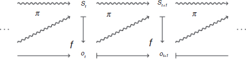
FIGURE B-2 A random dynamical system with complete connections.

models. In many cases, the hidden states are just independent random variables. It should be apparent—and this is the point of the figure and the preceding jargon—that at a formal level, an ABM is just another statistical model. Whatever is good or bad about ABMs lies in the details of their specification and implementation. Just to touch base with the high-level description, the inputs are o₀ and s₀ (which will itself be drawn from a given probability distribution), and the outcome is a probability distribution on the set of possible sequences (o₁, o₂, . . . , o_T), which is generated as described above. The parameters determine the probability distribution on outcome sequences through their effects on π and f. The o_t are high-dimensional objects that describe the current action or state of each agent. Emergent properties have to do with aggregates, such as the population mean and variance of behavior, and other less obvious functions of the observables. For example, in the SIS CAS, the extinction time is an emergent property.

REFERENCES

Borges, J. L. 1998. On exactitude in science. In Collected fictions. A. Hurley (Trans.). New York: Penguin Books. P. 325.

Cartwright, N. 1979. Causal laws and effective strategies. NOÛS 13:419–437.

———. 1989. Nature’s capacities and their measurement. Oxford, UK: Oxford University Press.

Eubank, S., H. Guclu, V. S. A. Kumar, M. V. Marathe, A. Srinivasan, Z. Toroczkai, and N. Wang. 2004. Modelling disease outbreaks in realistic urban social networks. Nature 429(6988):180–184.

Halpern, J. Y., and J. Pearl. 2005a. Causes and explanations: A structural-model approach. Part I: Causes. The British Journal for the Philosophy of Science 56(4):843–887.

———. 2005b. Causes and explanations: A structural-model approach. Part II: Explanations. The British Journal for the Philosophy of Science 56(4):889–911.

Heckman, J. J. 2000. Causal parameters and policy analysis in economics: A twentieth century retrospective. The Quarterly Journal of Economics 115(1):45–97.

Hoffer, L. D., G. Bobashev, and R. J. Morris. 2009. Researching a local heroin market as a complex adaptive system. American Journal of Community Psychology 44(3-4):273–286.

Holland, J. 1975. Adaptation in natural and artificial systems: An introductory analysis with applications to biology, control and artificial intelligence. 2nd ed. (1992). Cambridge, MA: MIT Press.

Hood, W. C. and T. C. Koopmans (Eds.). 1953. Studies in Econometric Method. Cowles Commission Monograph 14. New York: Wiley.

Hume, D. 1777. Enquiries concerning the human understanding, and concerning the principles of morals. Edited by L. A. Selby-Bigge. 2nd ed. (1902), Oxford, UK: Clarendon Press.

Iosifescu, M., and S. Grigorescu. 1990. Dependence with complete connections and its applications. Cambridge, UK: Cambridge University Press.

Lewis, D. 1973. Causation. The Journal of Philosophy 70(17):556–567.

Lucas, R. 1976. Econometric policy evaluation: A critique. In The Phillips Curve and labor markets, edited by K. Brunner and A. H. Meltzer. Amsterdam, Netherlands: North-Holland Publishing Company. Pp. 19–46.

Manski, C. F. 2010. Vaccination with partial knowledge of external effectiveness. Proceedings of the National Academy of Sciences of the United States of America 107(9):3953–3960.

———. 2011. Choosing treatment policies under ambiguity. Annual Review of Economics 3:25–49.

Marschak, J. 1974. Economic measurements for policy and prediction. In Economic information, decision, and prediction, Vol. 7–3. Netherlands: Springer. Pp. 293–322.

Milnor, J. 1954. Games against nature. In Decision processes, edited by R. M. Thrall, C. H. Coombs, and R. L. Davis. New York: Wiley. Pp. 49–60.

Norman, M. F. 1972. Markov processes and learning models. New York: Academic Press. http://public.eblib.com/choice/publicfullrecord.aspx?p=453098 (accessed November 17, 2014).

Pearl, J. 2009. Causality: Models, reasoning, and inference. 2nd ed. Cambridge, UK: Cambridge University Press.

Putnam, H. 1974. The “corroboration” of theories. In The philosophy of Karl Popper, edited by P. A. Schilpp. La Salle, IL: Open Court. Pp. 221–240.

Savage, L. 1954. The foundations of statistics. New York: Wiley.

Schelling, T. C. 1971. Dynamic models of segregation. Journal of Mathematical Sociology 1(2):143–186.

Simon, H. A. 1953. Causal ordering and identifiability. In Studies in econometric method, edited by W. C. Hood and T. C. Koopmans. New York: Wiley. Pp. 49–74.

Stoye, J. 2012. New perspectives on statistical decisions under ambiguity. Annual Review of Economics 4(1):257–282.

Tesfatsion, L. 2015. Verification and empirical validation of agent-based computational models. http://www2.econ.iastate.edu/tesfatsi/empvalid.htm (accessed November 17, 2014).

Tinbergen, J. 1968. Statistical testing of business-cycle theories. New York: Agathon Press.

Toroczkai, Z., and S. Eubank. 2005. Agent-based modeling as a decision-making tool: How to halt a smallpox epidemic. The Bridge 35(4):21–27.

Wright, S. 1921. Correlation and causation. Journal of Agricultural Research 20(7):557–585.

———. 1925. Corn and hog correlations. U.S. Department of Agriculture Department Bulletin 1300:1–60.

Young, H. P. 2001. Individual strategy and social structure: An evolutionary theory of institutions. Princeton, NJ: Princeton University Press.

This page intentionally left blank.