
This chapter reviews the hydrologic modeling used to support the Edwards Aquifer Habitat Conservation Plan (HCP). There are two primary objectives for these modeling efforts. The first objective is to create a model that can reproduce known spring flows, since habitat protection is dependent in part on adequate spring flow. Second, once a model has been developed that meets criteria for suitability, it can be used as a predictive tool. There are two types of predictions needed to support the HCP: (1) predicting the effects of future hydrologic conditions (such as climate change and droughts) on spring flow, and (2) predicting how management actions (like conservation measures) will affect water levels and spring flows. This chapter discusses the appropriateness of the hydrologic modeling strategies used for the Edwards Aquifer and it suggests additional analyses to quantify and, if possible, reduce uncertainty and improve defensibility.
Often information necessary for planning, operations, and design of water resources systems are either inadequate or unavailable at locations of interest. It is generally not feasible or cost-effective to perform field experiments to determine the response of the water resources systems to a range of proposed management actions. Thus, practitioners have turned to modeling as a way of predicting the future behavior of an existing or an altered hydrologic system (Loucks, 1990). Groundwater modeling in particular has become an important tool for planning and decision making
associated with groundwater management, which entails the efficient utilization of groundwater resources in response to current and future demands while protecting the integrity of the resource to sustain environmental needs (EPA, 1988).
Hydrologic simulation models entail the mathematical description of the components and the response of the hydrologic system to a series of events during a desired time period. All models are simplified representations of the system being modeled. The extent to which system complexity is incorporated depends on the skill of the modeler, the time and money available, and perhaps most importantly the modeler’s understanding of the real system (Loucks, 1990).
Modeling typically proceeds in phases. First a conceptual model is developed that, for a fractured rock system like the Edwards Aquifer, should include (a) identification of the most important boundary conditions and features of heterogeneity in the system; (b) identification and orientation of the most important conduit flow paths and fractures in the rock mass (which may indicate anisotropy); and (c) determination of how much water such features conduct. The conceptual model along with field observations and measurements are essential to selecting the best code for the model, which is the second major phase. The code should meet the requirements of the problem and should be verified to test that the code is functioning properly. Verification involves comparison of the model output to a known (analytical) solution; it is needed to ensure that the code performs as expected with minimal errors. Third, once data are collected for input into the model, model runs can be performed and the results should be compared to measured data, a phase called calibration. During calibration, the modeler selects parameters to adjust and determines the range of parameter values to test. Fourth, once a satisfactory calibration is achieved, the model should be run without adjusting the calibration parameters, and the output should be compared with a new data set not used during the calibration—a phase called validation.
The Committee recognizes the controversy over validating groundwater models of complex systems (see Anderson and Woessner, 1992; Konikow and Bredehoeft, 1992), much of which stems from the inherent difficulty of the task as well as from the inconsistent or unclear use of the term “validation.” To help alleviate some of the confusion, Beven and Young (2013) have recommended the term “conditional validation,” which implies that the conditions under which the model is being validated are made explicit and they may change in the future. According to these authors, models that have been conditionally validated “have immediate practical utility in simulating within the range of the calibration and evaluation data, while allowing for their updating in the light of future research and development.” This report uses the term “validation” to refer to testing of
the model’s predictive abilities against data that were not used during the calibration phase. Such testing is just one of many procedures that can be used to improve confidence in the model output, as discussed in the section on uncertainty analysis.
It should be noted that the Edwards Aquifer Authority (EAA) has sometimes used the term “verification” in several of their reports and presentations to the committee when describing model runs that started with existing parameters but allowed for changing parameters to update the model. This is not a typical use of the term verification, nor does it describe the process of validation, and it may confuse those who intend to use the models. Instead, these efforts are more accurately described as additional calibration runs. This distinction becomes important later in the chapter as we review the updates made to the MODFLOW model of the Edwards Aquifer.
GROUNDWATER FLOW MODELS OF THE EDWARDS AQUIFER
Modeling of flow and transport in systems with conduit flow such as the Edwards Aquifer requires the use of complex models in order to account for its unique hydrogeology, which is characterized by significant heterogeneity in both porosity and permeability (see Box 2-1). The modeling of any system requires the development of, and revisions to, a conceptual model that constitutes a hypothesis describing the main features of geology, hydrological setting, and site-specific relationships between geological structure and patterns of fluid flow.
Over the years, there have been several efforts to characterize the hydrostatigraphy of the Edwards Aquifer with a goal of developing a conceptual model (Maclay, 1995; Hovorka et al., 2004; Lindgren et al., 2004; Worthington, 2004). Lindgren and others (2004) offer a comprehensive literature review of hydrogeology, hydrogeochemistry and karst evolution of the Edwards Aquifer, including characterization of flow; spatial distributions of hydraulic conductivity, storage, and porosity; and delineation of aquifer boundaries. Multiple data sources were used to develop the 3D framework and characterize 3D properties of the Edwards Aquifer (e.g., Hovorka et al., 1995; Small et al., 1996; Collins, 2000; Mace, 2000), including surface geologic mapping, log analysis, aquifer testing and structural interpretations.
Most models of the Edwards Aquifer are based on the popular MODFLOW code (McDonald and Harbaugh, 1988; and subsequent versions such as Niswonger et al., 2011), developed by the U.S. Geological Survey (USGS). MODFLOW provides estimates of water levels and fluxes (such as spring flow) given inputs that include hydraulic conductivity, recharge, and pumping. It can be used for 2D or 3D flow and under transient
Box 2-1
Challenges of Modeling the Complex Hydrogeology in the Edwards Aquifer
The hydrostatigraphy of the Edwards Aquifer is extremely complex primarily due to the presence of the Balcones Fault Zone and karst system where soluble host rocks have dissolved preferentially to form large interconnected conduits (see Figure 2-1). A “conduit” is defined as a karst-aquifer feature that is similar to a pipe (>1 ft diameter) through which groundwater flows much more quickly than in the smaller pores and fractures of the surrounding rock. Conduits form by the dissolution of soluble rocks, such as limestone. A “conduit zone” is defined as set of parallel conduits in a group that together perform the same function as one larger conduit. Some models simulate conduits as pipe-flow features, where equations for fluid flow in pipes are used, as opposed to Darcian flow in a uniform porous matrix.
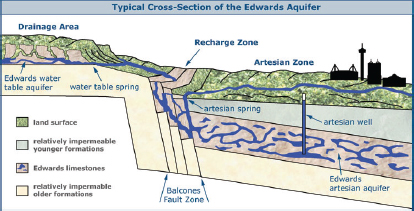
FIGURE 2-1 A simplified representation of a typical cross-section of the Edwards Aquifer.
SOURCE: http://www.edwardsaquifer.net/intro.html.
A fault is a fracture or fracture zone along which there has been displacement of two blocks of the earth’s crust or a geological formation. The effect of the fault zone on groundwater flow can be diverse; some faults enhance groundwater flow along the fault plane (and hence are preferential pathways), whereas others impede the flow of groundwater crossing the fault (and therefore are called barrier faults).
The extensive fault network in the Edwards Aquifer presents a modeling challenge. While numerous hydrologic studies involving conduit mapping and dye tracing have characterized the system, the nature and extent of spatial porosity and other properties is broadly interpreted in some areas. Hovorka et al. (2004) and Worthington (2004), for example, interpret potentiometric troughs to hypothesize a regional conduit flow system. Lindgren et al. (2004) also note “If flow feeding Comal Springs is dominated by a few large conduits, the few available aquifer tests do not characterize those conduits.” Further, Longley (1981) reports blind
catfish in a well at 1500 ft below land surface approximately 15 miles away from the recharge zone, suggesting rapid transport through large conduits.
A variety of classification systems exists for mathematical models of fractured aquifers with conduit flow (NRC, 1996; Cook, 2003; Schmelling and Ross, 2004; Bordas, 2005). They generally fall into one of two broad classes: (a) equivalent continuum models; and (b) discrete feature models (see Figure 2-2). In case of the equivalent continuum models, the heterogeneity in the fractured system is simulated using a limited number of regions, each approximated to be an equivalent porous medium (EPM) assuming uniform properties. Discrete network models, commonly known as discrete fracture network (DFN), characterize these features explicitly using such properties as aperture, orientation and length. The main motivation for DFN models is that, at every scale, flow is dominated by a limited number of discrete pathways formed by fractures or conduits (Dershowitz et al., 2004). The extensive data required for DFN models limit their use to sites with a relatively small number of well-defined structures (EPA, 1989). In many cases, the features controlling flow are not known at the scales necessary for modeling. In such instances the stochastic modeling approach in which the physical parameters are described as a random field characterized by a probability distribution may be used (Cook, 2003).
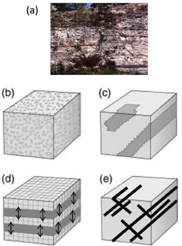
FIGURE 2-2 Different modeling approaches for fractured rock aquifers. These approaches are analogous in karst, and the figure has been modified to show karst approaches. (a) Photograph of an actual karst network; (b) Equivalent porous media model, using uniform aquifer parameters; (c) Equivalent porous media model in which highly fractured zones such as shown in (e) are represented by regions of higher hydraulic conductivity; (d) Dual continuum model in which the matrix and hypothetical high permeability layer or boundary interact through an exchange term (arrows); (e) Discrete fracture or pipe model, in which the major conduits are explicitly modeled; for karst, these discrete features would be pipe-like.
SOURCE: Adapted from Cook (2003).
conditions (e.g., to evaluate changes in recharge or pumping over time). Most of the Edwards Aquifer models developed so far have used an equivalent porous media (EPM) approach in which aquifer regions are assumed to have uniform aquifer parameters, rather than incorporating karst features. Table 2-1 lists the various numerical models of the Edwards Aquifer, noting how they dealt with karst features. Lindgren et al. (2004) modeled conduits using high permeability zones. Painter et al. (2007) along with Sun et al. (2005) used a version of MODFLOW with a conduit package.
Improvements in model design to facilitate the implementation of the Habitat Conservation Plan (HCP) have led to the last three modeling efforts listed in Table 2-1. The improvements include simulated transient water levels, better aquifer characterization and boundary conditions, new methods for determining recharge and water budgets, and more accurate calibration to springs. The first major modeling activity is that the EAA has added calibration data to develop a 2014 version of the MODFLOW model and used it to test management strategies that are major components of the HCP (discussed further below). Second, the HCP requires a new model of the Edwards Aquifer to be developed and ready for use by December 31, 2014, and expects it to be a finite element (FE) model. To satisfy the second requirement, the EAA contracted with the Southwest Research Institute (SwRI) to develop a new FE groundwater model of the Edwards Aquifer over a 3-year period. The Scope of Work for the FE modeling specified certain requirements including improvements to the conceptual design, boundary conditions, structure of the model (e.g., inclusion of conduits in the groundwater system), and model performances including calibration targets. The model development effort also included a Groundwater Model Review Panel (GMRP) to provide technical assistance and oversight.
The EAA’s 2014 MODFLOW model is a single layer transient flow model to simulate heads and spring flows (HDR, 2011; EAA presentations to the NRC Committee). This version extends from Las Moras Springs near Bracketville in the west to San Marcos Springs in the east. Some versions of the model (Table 2-1) extend east to Barton Springs, but a groundwater divide has been identified between San Marcos and Barton Springs, such that Barton Springs can be considered to be in a separate groundwater basin. The model is bounded on the north by the extent of the Edwards Aquifer outcrop and on the south by the saline zone. Thus, the model area includes the confined and unconfined Edwards Aquifer, but not the contributing area where recharge may enter the Trinity Aquifer and cross over to the Edwards Aquifer (see Figure 2-3).
The EAA’s 2014 MODFLOW model was first calibrated using data
TABLE 2-1 Numerical Groundwater Flow Models of the Edwards Aquifer
| Model Code | Geographical extent | Authors | Comments about model structure and conduits |
| GWSIM | San Antonio segment | Klemt et al. (1979) | EPM |
| GWSIM | San Antonio segment | Thorkildsen and McElhaney, 1992 | Revision of Klemt et al. (1979); EPM |
| MODFLOW | Barton Springs segment | Scanlon et al. (2002) | EPM |
| MODFLOW | San Antonio and Barton Springs segments | Lindgren et al. (2004) | Incorporated lines of EPM cells with high K for conduits |
| MODFLOW | Barton Springs segment | Smith and Hunt (2004) | Revision of Scanlon et al. (2002); EPM |
| MODFLOW | San Antonio and Barton Springs segments | Lindgren (2006) | Revision of Lindgren et al. (2004) with wide zones of EPM cells for conduits |
| MODFLOW-DCM | Barton Springs segment | Painter et al. (2007); Sun et al. (2005) | Dual conductivity model (dual porosity type) |
| EAA 2014 MODFLOW | San Antonio segment | Winterlee 2014a | Revision of Lindgren et al. (2004) that includes zones of cells with high K for conduits in limited areas |
| TRANSIN | Edwards Aquifer | SWRI (ongoing) | Finite-element model using the EPM approach |
| FEFLOW | Edwards Aquifer | SWRI (ongoing) | EPM (as of May 2014) |
NOTE: EPM, equivalent porous media; K, hydraulic conductivity.
from 1941 to 2000, then recently recalibrated using data from 2001 to 2009. The recent efforts took advantage of new pumping data for 2,719 permitted wells. Rather than using the parameters from the previous modeling period, additional adjustments were made to recharge and initial water levels to improve the match for the 2001-2009 calibration. Several different data sets from December 1973 to December 2000 were used for the initial head, and the recharge was also varied using the original and eight different adjustments (see Table 2-2).
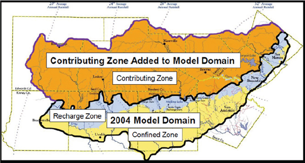
FIGURE 2-3 This map of the Edwards Aquifer region shows the 2004 model domain used in the MODFLOW model as well as the expanded domain used for the finite element model that includes the contributing zone.
SOURCE: Winterlee (2014a).
TABLE 2-2 Modifications to recharge tested during 2014 MODFLOW runs to calibrate to the 2001-2009 data set. Note that although the table refers to “verification run,” these efforts were not “verification” but another calibration.
| Verification Run# | Recharge Data Set | Initial Head Distribution |
| 1 | Adjusted Recharge & Blanco R Recharge Peak Cut | Dec-00 |
| 2 | Adjusted Recharge & Blanco R Recharge Peak Cut | Nov-00 |
| 3 | Adjusted Recharge & Blanco R Recharge Peak Cut | Dec-78 |
| 4 | Adjusted Recharge & Blanco R Recharge Peak Cut | Dec-73 |
| 5 | USGS Estimated Recharge Deliverable (by Puente, 1978) | Dec-78 |
| 5-2 | USGS Estimated Recharge (by Puente, 1978) | Jun-76 |
| 6 | Adjusted Recharge (after Lindgren et al., 2004) | Dec-78 |
| 6-2 | Adjusted Recharge (after Lindgren et al., 2004) | Jun-76 |
| 7 | Adjusted Recharge & Blanco R Recharge Peak Cut | Dec-78 |
| 7-2 | Adjusted Recharge & Blanco R Recharge Peak Cut | Jun-76 |
| 8 | Leona Springs Property Changes with Adjusted Recharge & Blanco R Recharge Peak Cut | Dec-78 |
| 9 | Adjusted Recharge & Blanco Recharge Cut + Barton Springs Segment Elimination | Dec-78 |
| 9-2 | Adjusted Recharge & Blanco Recharge Cut + Barton Springs Segment Elimination | Jun-76 |
| 10 | Adjusted Recharge & Blanco Recharge Cut at Daily Time-step Simulation | Dec-78 |
| 10-2 | Adjusted Recharge & Blanco Recharge Cut at Daily Time-step Simulation | Jun-76 |
| 11 | Adjusted Recharge & Blanco Recharge Cut- Run with Newton-Raphson Solver | Dec-78 |
| 11-2 | Adjusted Recharge & Blanco Recharge Cut- Run with Newton-Raphson Solver | Jun-76 |
SOURCE: Winterlee (2014b).
The model predicts water level to compare with 423 observation wells and spring flow at seven targets distributed from east to west across the aquifer. The well targets are distributed across both the recharge zone and the confined zone of the aquifer, but with higher density in the eastern third of the aquifer. Distributing the calibration targets strengthens the model calibration. Model results were compared to monthly measurements, which is the finest timescale used in this modeling.
Some observations from these calibrations (found in Winterlee, 2014c) illustrate both the strengths and weaknesses of the modeling. Spring flow at Comal Springs tended to have better fits than at San Marcos Springs; Well J-17 was better than Well J-27, and the well water levels had better fits than the spring flows. Linear correlation coefficients (R2) between observed and modeled heads and spring flows varied between 0.5 to 0.9. Modeled spring flows between 1947 and 2000 for San Marcos and Comal Springs were presented for both a diffuse and a conduit model. The residuals between observed and modeled flows varied over the time period but commonly reached 50 to 100 cfs (positive or negative), which is of the order of the minimum springs flow objectives in the HCP. Both the conduit and diffuse models tended to underpredict low flows at San Marcos Springs, although the fit improved in the last decade of the modeling period, from errors of 50 cfs to 10 cfs or less (Figure 2-4). High flows were both under- and over-predicted. At Comal Springs, the conduit model tended to overpredict the low flows by 10 to 20 cfs in the period after 1976 (Figure 2-5). The diffuse model fit low flows better in this time period. For high flows at Comal, both under- and over-prediction were observed and the conduit model tended to have higher flows at the peak than the diffuse model. Conceptually, conduit flow models should provide faster flow of water from west to east and improve short term responses such as peaks and low flows or response to changes in recharge. Further discussion of how conduits and barriers are used in the model is in a following section.
The MODFLOW model was used to test management scenarios under conditions intended to replicate the drought of record (Figure 2-6). The simulations show that the highest level of mitigation was needed to keep the spring flow at Comal Springs above 30 cfs (Figure 2-7). That is, voluntary irrigation suspension (VISPO), municipal water conservation (Conservation), aquifer storage and recovery (San Antonio Water System [SAWS] ASR) and Stage V emergency reductions (Stage V) were all needed, with ASR making the largest contribution to predicted spring flows.
Although the MODFLOW model has provided a valuable tool for improved understanding of the Edwards Aquifer flow system and evaluation of management scenarios, there is uncertainty about the accuracy of the model predictions for a number of reasons. First, uncertainties in recharge and pumping can hamper calibration. For example, the lack of detailed in-
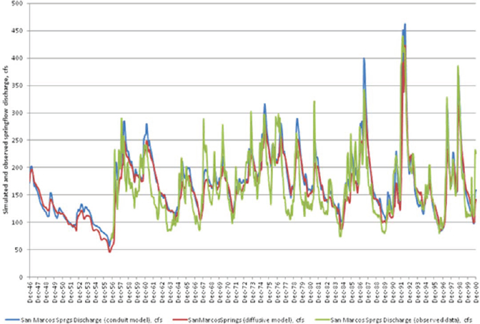
FIGURE 2-4 Actual and predicted San Marcos spring flow, comparing the EAA 2014 MODFLOW model (labeled the conduit model) and the older USGS MODFLOW model of Lindgren (2006) (labeled the diffuse model).
SOURCE: Winterlee (2014c) Slide 64.
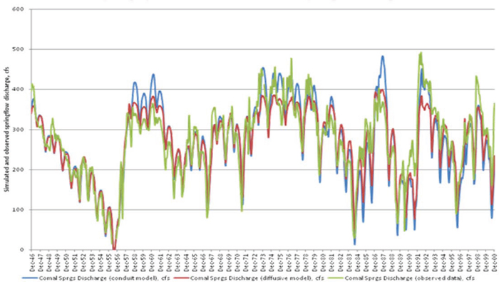
FIGURE 2-5 Actual and predicted Comal spring flow, comparing the EAA 2014 MODFLOW model (labeled the conduit model) and the older USGS MODFLOW model of Lindgren (2006) (labeled the diffuse model).
SOURCE: Winterlee (2014c) Slide 66.
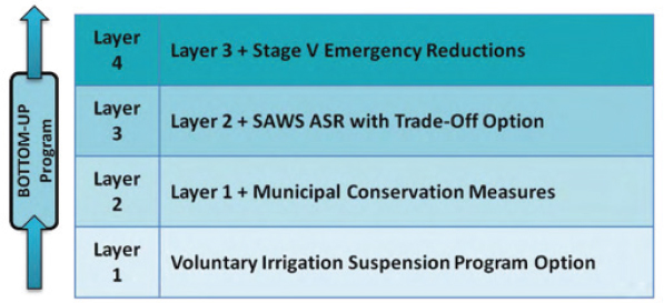
FIGURE 2-6 Spring flow protection measures in the HCP and included in the MODFLOW model. The actual numerical changes made to pumping or additional inputs required to represent the four spring flow protection measures were not provided.
SOURCE: Winterlee (2014a).
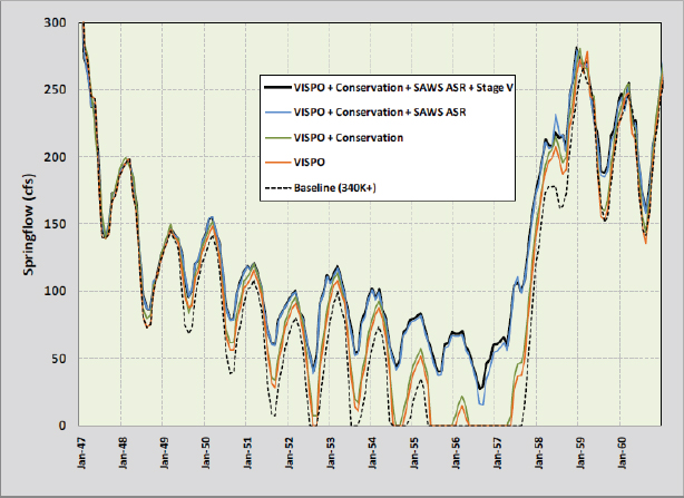
FIGURE 2-7 Modeling runs from the HRD report (Appendix K of the HCP) showing predicted Comal Springs discharge under the different management scenarios shown in Figure 2-6.
SOURCE: Winterlee (2014a) and EARIP (2012).
formation on pumping in the extensive well network of the Edwards region has limited the time-step size for transient modeling to monthly time steps, which in turn may limit the ability of the model to provide daily predictions for the HCP. Second, there is uncertainty in every model about heterogeneity in hydraulic conductivity, but this can be particularly troublesome for karst aquifers. There has been debate among those involved in modeling the Edward Aquifer about how to model karst conduits as well as fault barriers, both of which are important to producing a well-calibrated model. Third, the lack of a validation period for the MODFLOW model limits the confidence in model predictions. Fourth, there has been little documented uncertainty or sensitivity analysis for the MODFLOW model, although many techniques are available and are discussed further below. Finally, the scenario testing has thus far been limited to the drought of record. The model does not need to be limited to this scenario and one of the benefits of modeling is evaluating multiple factors including potentially more severe system stressors.
It is clear that extensive work has been conducted to model the Edwards Aquifer. Given the large scale and complexity of the aquifer, it is likely that data limitations and conceptual model issues will continue to arise. Thus, the MODFLOW modeling effort should be viewed as a work in progress and not a final product.
Finite Element Model Development
At the time of the writing of this report, development of a finite element (FE) model of the Edwards Aquifer is under way using the FEFLOW code. The purpose of developing an alternate groundwater model, according to the HCP, is to reduce uncertainty in the modeling results and increase the reliability and the defensibility of the model projections of aquifer and spring flows. Another reason for developing a second model of the Edwards Aquifer, although this is not stated in the HCP, would be to capitalize on the unique features available in FEFLOW. The finite element model is more appropriate for aquifers with complex hydrostratigraphy because it is not limited by the rectangular model cells typically used in finite difference models such as MODFLOW. In addition, standard MODFLOW models represent the porous medium as having relatively slow laminar flow, whereas the flows in the conduit networks such as those found in the Edwards Aquifer may occur under turbulent conditions. Some of the recent finite element models of groundwater systems allow the users to simulate turbulent flow in conduits, such that the simulation of fate and transport of flow and contaminants in such models are deemed more accurate for systems where both laminar and turbulent flows are present. The treatment of discrete flow features in FEFLOW is quite comprehensive, allowing the user to imple-
ment a variety of geometries, phreatic and non-phreatic conditions, as well as three flow types using Darcy, Hagen-Poiseuille, and Mannings-Strickler equations. Various forms of flow equations used in FEFLOW enables it to simulate flow through porous media, pressure flow through geometries idealized as pipes or parallel plates, and open channel flow in both surface and subsurface features. FEFLOW’s capability for modeling anisotropy and discrete flow features (Diersch, 2014) has been demonstrated in the Florida Aquifer in North Florida (Meyer et al., 2008).
In support of the finite element model, SwRI was also asked to further refine conceptualization of the Edwards Aquifer. Some of the suggested model improvements described in the statement of work include (Green et al., 2014):
- expansion of the model domain to include the contributing zone
- refinement of boundary conditions
- development of a refined hydrostratigraphic framework model, fault and conduit characterization
- correlation analyses to quantify the relationship between recharge events and aquifer response
- characterization and measurement of discharge mechanisms including paleo-stream underflow
- inclusion of both conduit and diffuse flow
These refinements are appropriate goals and could be applied to other Edwards Aquifer models as well. Not all of these refinements had been incorporated into the models as of the May 2014 presentation to the Committee.
The following brief assessment of the FE modeling effort is based primarily on presentations from SWRI as well as progress reports of model development to the EAA (completed in May 2013, November 2013, and February 2014). Suggested improvements to the conceptual model are discussed in a later section on Future Directions, since they are not specific to FEFLOW.
As of May 2014, the FEFLOW model consists of about 50,000 elements. It was originally constructed using the finite element code TRANSIN and was then converted to FEFLOW. The current model uses the same equivalent porous medium (EPM) approach that was applied in the EAA 2014 MODFLOW model; that is, high transmissivity zones are being incorporated to model rapid flow movement in known conduits. The FEFLOW model covers a much larger area, including the Trinity Aquifer to the north, to better account for cross aquifer contributions (see Figure 2-3). [The Trinity Aquifer has a lower permeability than the Edwards, such that most recharge into the Edwards is occurring instead through the outcrop of
the Edwards Aquifer. Nonetheless, some recharge through the Trinity may occur based on water budgets (Mace et al., 2000 reported in Lindgren et al., 2004) and geochemical mixing models (Musgrove and Crowe, 2012).] The FE model has a time step of one month, although there have not been any studies to determine if this is adequate to simulate the rapid transfer of flow from source areas to springs that are of interest. The period of calibration is 2002 to 2011.
Because modeling was still in progress during the review period for this report, the Committee can say little about the results of the modeling efforts. However, it can address the stated purpose of having another groundwater model, which was to make comparisons between the MODFLOW and FEFLOW model results and thereby reduce uncertainty. This purpose cannot be achieved under the current modeling strategy. The two models, developed using two separate codes, will each have their own inherent uncertainty, which cannot be understood by a comparison of the two. Rather, uncertainty should be addressed using a variety of methods that are discussed extensively below. The two models could be used to compare differing recharge strategies, but the same could have been achieved by continuing to use only MODFLOW. Theoretically, the complex and nonlinear features of the fractured system of the Edwards Aquifer can be represented more accurately using a finite element mesh, but no such plans were presented to the Committee, and similar features are available in upgrades to MODFLOW (see MODFLOW-USG discussion below).
Importance of Conduits in Modeling Karst Aquifers
One of the key questions and a topic of extensive discussion is how conduit flow should be represented in Edwards Aquifer models. Differing opinions exist within the public, water-management, and scientific communities about whether there is enough evidence to support the placement of conduits in the model and, if so, how it should be done.
Several lines of evidence suggest the importance of conduits in this system. Localized dye tracings indicate very high water velocities in the subsurface, and additional dye tracing is under way (Johnson et al., 2012). Flashy responses in wells and springs are also evidence of conduit flow. Lindgren et al. (2009) discussed improved model fits at high and low flows when conduits are included.
The current EAA MODFLOW model, originally constructed by the USGS (Lindgren et al., 2004) and later revised by the EAA (HDR, 2011), simulates conduits in selected areas with zones or rows of finite-difference, Darcian-flow cells with anomalously high permeability. This conceptualization is illustrated in Figure 2-2c. The simulated conduits in the model by Lindgren et al. (2004) were 0.25 miles wide, or the width of a model
cell. Although this is much wider than actual conduits in the aquifer, these features were narrow relative to the scale of the model area and were used to simulate the general characteristics of a conduit system rather than the specific physical processes of flow in actual karst dissolution features. Fluid flow in these zoned features was simulated in the same way as in the surrounding cells, except with higher permeability, although not reaching a true conduit velocity.
Several other methods of representing conduits in the models are possible. Pipe or line elements are small features with conduit properties inserted at discrete locations as indicated by Figure 2-2e. These pipes simulate flow on the basis of laminar flow equations with high velocity; also, turbulent flow is now available or in development for certain codes. The pipes simulate open-channel flow when not fully saturated. Within such models, the locations of both high velocity features and contrasting fault barriers are highly uncertain. Another option for representing conduits is to treat their locations as uncertain but just provide dual permeability in representative layers (Panday et al., 2013) as illustrated in Figure 2-2d. The dual permeability model nonetheless requires characterization of each media (the matrix and the higher permeability conduit zone) and an exchange term for communication between the layers. A final option is to use an equivalent porous media (Figure 2-2b) with a slightly higher permeability than rock without conduits and perhaps some anisotropy if there is a preferential flow direction.
The model presentations to the Committee do not make it clear to what extent conduits have been included in the current modeling, and controversy surrounds the choice of method. The use of conduit features that are larger than observed to approximate the behavior of conduits seems unrealistic and raises concern that they might overestimate conduit behavior. The EAA also indicated that the locations of such features are non-unique in model calibration, which makes the model open for criticism (EAA/NRC, 2014). Despite this, the Committee feels that the rapid aquifer response to recharge and management actions will not be adequately simulated without the use of conduit-like features, especially if the modeling effort moves to a shorter time step in the future (see subsequent discussion).
Both the MODFLOW and FEFLOW modeling efforts presented to the Committee have showed a high level of sophistication and considerable effort to capture the complex flow system of the Edwards Aquifer. The Committee has a number of suggestions (1) about changes being made to the conceptual model and (2) to help quantify uncertainty and increase the ability of the models to make predictions.
Continue Improvements in Recharge Estimates
Groundwater recharge from the land surface (hereafter, recharge) is the most sensitive parameter affecting spring flow for normal or above normal precipitation periods (Lindgren et al., 2004). Given the importance of recharge for a groundwater system, improving the accuracy of recharge estimates has the potential to improve the model considerably. Recharge to the Edwards Aquifer occurs through groundwater infiltration of streams that cross the recharge zone and from direct precipitation on the recharge zone (Puente, 1978; Lindgren et al., 2004; EAA, 2013). Additionally, the EAA operates four structures within the Edwards Aquifer recharge zone that capture runoff and induce groundwater recharge as described in EAA (2013).
The original Edwards Aquifer model (Lindgren et al., 2004) and subsequent MODFLOW efforts (EAA, 2013) have all relied on a method for estimating recharge described by Puente (1978). The Puente method uses streamflow measurements upstream and downstream from the recharge zone and estimates tributary inflow to determine stream recharge on a monthly basis; this method also estimates base flow and recharge from direct precipitation. Evapotranspiration is neglected in this method, but this has been deemed acceptable because much of the recharge comes from large storms for which evapotranspiration is negligible (personal communication, Richard Slattery, USGS, 2014). Recharge estimates from the Puente method were applied to a model “testing period” that followed the calibration period, which was an attempt at model validation (Lindgren et al., 2004); however additional parameter adjustments were needed for this testing period, and therefore, the model was not truly validated. This raises questions about the accuracy of the recharge estimates.
Currently, the EAA is developing an improved method to estimate recharge by application of the Hydrological Simulation Program—Fortran (HSPF; http://water.usgs.gov/software/HSPF/; accessed December 5, 2014). HSPF is a watershed streamflow model that simulates continuous streamflow resulting from system inputs of continuous precipitation and other meteorological data. HSPF also simulates soil moisture, overland surface runoff from rainfall, shallow groundwater flow toward streams (interflow), groundwater inflow to streams (base flow), snowpack depth and water content, snowmelt, evapotranspiration, groundwater recharge, stream channel routing, reservoir routing, and water-quality parameters. The Puente method does not account for most of these processes and, therefore, is much simpler than HSPF. If the HSPF model is calibrated to observed streamflow, the component of groundwater recharge simulated by HSPF can be used as an estimate of groundwater recharge for the Edwards Aquifer groundwater-flow models. Also, the HSPF model can be used to estimate
streamflow entering the Edwards Aquifer recharge zone from the north, a function that cannot be performed with the Puente method but would be necessary to estimate recharge for a hypothetical precipitation scenario, such as drought.
It is important that the parameters of the HSPF model be consistent with the intricacies of a karst system (Ford and Williams, 2007). The recharge zone for the Edwards Aquifer consists of karst rocks that allow fast infiltration of precipitation and surface water through fractures and dissolution openings such as caves. Streams flow onto the Edwards Aquifer recharge zone from the north (Edwards Plateau) and sink into the Edwards Aquifer (Puente, 1978). A stream that sinks into the ground indicates that the groundwater table is below the streambed, and, if possible, the parameters of the HSPF model should be set accordingly to allow fast infiltration of surface water. Accurately estimating the temporal changes in recharge is essential for simulating changes in spring flow.
Clear Creek Solutions, Inc. (2012, 2013) has used HSPF to simulate streamflow for selected sub-basins that contribute to the Edwards Aquifer in order to estimate groundwater recharge. Results from this modeling have been compared to use of the Puente method for estimating recharge, as shown in Figure 2-8. Note that there are large differences in the recharge estimates, especially at higher recharge values. The Committee recommends continued development and testing of the HSPF model for estimating recharge. Uncertainty analysis, as discussed in a subsequent section, will provide guidance as to which recharge method to use.
Improve Conduit Representation
As stated previously there are a range of options for representing conduits, from no conduits to discrete pipe flow simulation with high velocity paths (Figure 2-2). Given the evidence that conduits play a role in karst aquifers such as the Edwards, it is suggested that conduits be represented in the model to a greater degree than what was presented to the Committee, despite uncertainty about conduit locations, diameters, lengths, and other properties. Uncertainty is associated with all model features, and can be evaluated using uncertainty analysis (discussed in the following section).
Although the EAA currently does not have an objective to accurately simulate groundwater velocities measured from dye tracing, this capability would enhance the defensibility of a model and thus would be a useful long-term goal—one in which conduits will be necessary. The ability to simulate these flow velocities in future models also would allow the simulation of current or potential transport of contaminants to the springs, such as herbicides, insecticides, and volatile organic compounds frequently detected in Barton Springs (Mahler et al., 2006). Groundwater-age dating and analysis
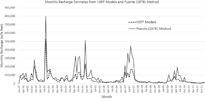
FIGURE 2-8 Comparison of recharge estimates from the Puente method and HSPF.
SOURCE: Winterlee (2014d).
of specific conductance are other possible methods that could help to estimate conduit locations (Long et al., 2008).
A great deal of work has already been conducted to better identify and characterize conduits, both in terms of modeling and field programs such as tracer tests. The Committee reiterates the need to continue attempts to characterize conduits and determine their importance in discharge predictions from hydrologic models of the Edwards Aquifer. This notion was recently reinforced by the Groundwater Modeling Review Panel to the EAA, who recommended adding conduits to the finite element model (Saar, 2014). Conduits will become even more important for simulating daily spring flows with future models that have daily time steps (see later discussion on time steps). Effective communication to the public concerning the importance of conduits despite the uncertainty of conduit locations will be needed.
Uncertainty Analysis
All models have some level of error in their predictions. Quantifying this uncertainty, although a challenging task in many cases, increases the model’s defensibility and can provide a reasonable estimate of model error, which is important information when using a model for management decisions. In none of the presentations to the Committee have the results of the MODFLOW model been presented with errors bars or some other indication of the uncertainty in the predictions. Although EAA staff say that they intend to formally account for uncertainty, no document has been created laying out the methods. Furthermore, given that the calibration errors observed for the MODFLOW model are as large as the minimum required spring flows in the HCP, it is imperative to better understand model and input uncertainties and how they translate into uncertainties in the simulated management actions. Hence, this section describes ways for the EAA to formally consider uncertainty in their hydrologic models, both for MODFLOW and the finite element model.
In the section below, quantitative methods are described that can assess (1) the uncertainty of individual parameters, groups of parameters, or the nonlinear interactions thereof (parametric uncertainty); (2) the uncertainty of model predictions (predictive uncertainty); and (3) the uncertainty associated with how the groundwater system is conceptualized (conceptual model uncertainty). There are other types of uncertainty that are not discussed here, including the uncertainty associated with the accuracy and fidelity of numerical algorithms chosen for the model and the measurement uncertainty associated with the data used to calibrate and validate the numerical models. In the Committee’s opinion, these latter types of uncertainty are likely to be of lower magnitude and less important to improv-
ing the current modeling effort of the Edwards Aquifer. The focus here is on methods that members of the Committee have found useful in similar systems. To be most useful for EAA managers, they are presented in order from easiest-to-implement to most complex: sensitivity analysis, formal model validation, PEST predictive uncertainty analysis, and the ensemble method. Some of these methods can address multiple types of uncertainty, as will be discussed. The section ends by discussing the reduction in predictive uncertainty that could result if new data were collected and what those data should include.
Sensitivity Analysis
Parameter sensitivity analysis is helpful in assessing model uncertainty quantitatively because large parameter sensitivity commonly results in large model uncertainty related to those parameters. If a parameter has large inherent uncertainty but the model is not sensitive to it, then the uncertainty of that parameter might not be critical. An example of this situation is where inflow from another aquifer has large inherent uncertainty but accounts for only a small component of total system inflow. For example, inflow to the Edwards Aquifer from the Trinity Aquifer is estimated to be 12,000 acre-feet per year but with a large uncertainty, ranging from 2,000 to 30,000 acre-feet per year. If this range is equivalent to only about 0.3 to 5 percent of the total aquifer inflow, the model would not be highly sensitive within this range. If, however, a parameter has large inherent uncertainty and also results in large model sensitivity, then that parameter is critical and contributes substantially to model uncertainty.
Although the original MODFLOW model (Lindgren et al., 2004) included a sensitivity analysis, none appears to be associated with either of the current models in progress. According to the EAA’s presentation to the Committee in May 2014, model parameters in the western part of the model and groundwater exchange with other aquifers are thought to account for the largest inherent parameter uncertainty. A well-designed, formalized sensitivity analysis could be used to indicate the model sensitivity to these parameters as varied within the ranges of their inherent uncertainty (e.g., Campbell and Coes, 2010). For example, each parameter or group of parameters could be increased by 1 percent, and the resulting change in spring flow at each spring of interest could be quantified. Parameter categories that should be included in a sensitivity analysis are recharge, horizontal and vertical hydraulic conductivity (Kh and Kv), spring conductance values that influence the rate of spring flow, and those related to fracture flow, conduit flow, and barrier faults, if applicable. A generalized sensitivity analysis might consist of only these parameter categories, where all model values within each category are varied as a group for the entire
model area, and the sensitivity by category is reported. In addition, more detailed approaches might include testing the sensitivity of individual spring conductances and Kh or Kv within subdivided model areas with respect to individual springs, especially for those of particular interest. In addition to varying all parameters equally, a plausible range for particular parameters of interest might be estimated in terms of the inherent uncertainty, as previously described. An interim detailed sensitivity analysis for the current MODFLOW model would provide additional guidance on calibration and how to better focus continued hydrogeologic characterization efforts. SENSAN is a utility that automates the tedious effort that is otherwise required to do sensitivity analysis (Doherty, 2005).
The simple sensitivity analysis discussed above, sometimes referred to as “one factor at a time” (OAT), is a useful general assessment but has the major limitation of neglecting nonlinear parameter interactions. To account for these interactions, and thus provide a better assessment of the relative parameter sensitivities, the Morris method can first be used to identify the most sensitive parameters, which then are evaluated in depth by the FAST method (Morris, 1991; Saltelli, 1999; Muñoz-Carpena et al., 2007; Srivastava et al., 2014). Nonlinear parameter interactions also can be assessed by methods described in Doherty et al. (2010) that, additionally, quantify predictive uncertainty, as discussed below.
Formalizing Model Validation
Validation refers to executing a calibrated model for a period of the data record not used in the calibration and comparing the results to measured data (e.g., groundwater levels and spring flows). The model’s goodness of fit to data for this period provides an estimate of the model’s predictive accuracy for simulation of a stress scenario, such as increases in pumping or drought, for a period of time equal to the validation period. This validation is conditional until future data are collected and tested with the model. If the predictive accuracy determined by validation is considered unacceptable for the EAA’s management purposes, then selected conceptual-model assumptions should be adjusted in the numerical model, which would then require recalibration (e.g., see Long and Mahler, 2013).
The MODFLOW model described by Lindgren et al. (2004) was calibrated to data for 1947 to 1990, and there was an attempt to validate the model to data for 1991 to 2000 (i.e., the “testing period”). Unfortunately, during this exercise additional adjustments to storativity and hydraulic conductivity values were made for areas near recharge zones, such that this was merely additional model calibration, not validation. The EAA’s current MODFLOW model was calibrated to data for 1941 to 2000, and again an attempt was made to validate the model to additional data for 2001 to
2009 (Winterlee, 2014b). However, further adjustments to recharge rates were made for this period to achieve an acceptable model fit, and similarly to Lindgren et al. (2004), this was merely additional model calibration. Having a validated model will allow the EAA to make better predictions of spring flow or groundwater-level responses for future scenarios. Box 2-2 describes how to determine confidence intervals based on validation-period residuals in order to quantify model uncertainty.
Box 2-2
Confidence Intervals Based on Validation-Period Residuals
Information about model uncertainty can be gained by estimating confidence intervals on the model validation, based on validation-period residuals. During validation, the residuals (or differences) between simulated and observed values are evaluated. A variety of metrics have been used for residuals in past Edwards Aquifer modeling efforts. For example, Lindgren et al. (2004) reported the mean absolute difference, mean algebraic difference, and root mean square (RMS) error of these residuals for single water-level measurements and water-level and spring flow time-series data. The EAA reported the correlation coefficient for water-level and spring flow time-series data for the 2001-2009 simulation (Winterlee, 2014b). All of these metrics are useful for a data set of single measurements or for a mixture of single measurements and time-series data; however there are other metrics that are more informative when assessing a simulated time-series record. The Nash-Sutcliffe coefficient of efficiency (E) (Nash and Sutcliffe, 1970; Legates and McCabe, 1999; Long and Mahler, 2013) is a useful measure of the similarity between simulated and observed time-series records. This metric compares the magnitude of residuals to the overall variability in the observed record and, therefore, puts these residuals in a meaningful context.
The validation-period residuals can be used to estimate confidence intervals on the model validation and thus convey information about model uncertainty. The first step is to calculate the standard deviation σ of all the residuals for the validation period. Then, plot the 95% confidence intervals for the validation period, which are at a distance of σ above and below the simulated spring flow. This assumes that the residuals are normally distributed and random. If, however, there is a relation between the magnitudes of residuals and the observation values (i.e., not random), then confidence intervals might be different for high, medium, and low flows, and these three categories could be plotted separately. These calculated confidence intervals can then be placed on simulated spring flow records for stress scenarios to show uncertainty of model predictions. It should be noted that these confidence intervals only apply to climatic, spring flow, and water-level conditions that are within historical ranges. Outside of these ranges the confidence intervals may be larger than those estimated. Also, these confidence intervals would be less certain for a prediction that extends beyond the length of the validation period.
PEST Predictive Uncertainty Analysis
PEST predictive uncertainty analysis, described by Doherty et al. (2010), requires that the inherent parameter uncertainty (i.e., range of each parameter’s potential values) be estimated on the basis of expert knowledge. This parameter uncertainty is then propagated to model predictions, such as changes in spring flow in response to changing climatic conditions or increased groundwater withdrawals, which can provide an estimate of confidence intervals on predictions. The method is based on the assumption that model outputs are linearly related to model-input parameters, although nonlinear relationships can also be handled via null-space Monte Carlo analysis (Tonkin and Doherty, 2009) but are more computationally intense. For example, uncertainty of the average recharge rate might, by expert knowledge, be determined to be within ±10% of that estimated by HPSF modeling. A recharge multiplier could then be applied in the groundwater model to the overall estimated recharge and allowed to vary by ±10% for the PEST predictive uncertainty analysis. Similarly, potential variability ranges could be estimated for all other calibrated parameters, such as hydraulic conductivity, storage coefficient, specific yield, and specified inflows or outflows. In the PEST uncertainty analysis, the potential variabilities of all model parameters are analyzed simultaneously. Plans to incorporate PEST into the current modeling efforts were mentioned by EAA scientists, but no results were available for the Committee to review.
Ensemble Method
Another source of uncertainty is associated with the assumptions in the conceptual model. A comparison of different sets of conceptual-model assumptions in different versions of the same model code (i.e., an ensemble) can be useful in quantifying this uncertainty. The ultimate goal of this exercise is to select from the ensemble the model version that best answers management questions. The ensemble method is similar to the PEST predictive uncertainty analysis previously described, except that conceptual-model assumptions are tested rather than parameter values. Hartmann et al. (2013) and Long and Mahler (2013) describe this method of testing multiple conceptual models of karst aquifers.
One application of the ensemble method useful for the Edwards Aquifer would be to assess the uncertainty associated with the precise locations and characteristics of conduits. Conduits might primarily be large, single features, or they might be smaller features that are grouped into conduit zones. Thus, conduits could be simulated by large, discrete pipe-flow features but also could be represented by wider zones having high Kh values; these two differing assumptions could be tested in different model versions.
Varying a conduit’s location to the right or left (perpendicular to flow) in different model versions could be used to test its optimum location and to indicate the zone within which a simulated conduit can be moved without adversely affecting the goodness of fit. This zone could be shown on a map of the model area, possibly as error bars placed perpendicular to the conduit, to indicate uncertainty of the conduit’s location. Also, the overall conduit network configuration in the model domain could be tested by placing conduits in many different plausible locations or by generating different conduit networks stochastically, as described by Ronayne (2013).
The ensemble method can also be used to assess predictive uncertainty by comparing the model outputs from all plausible model versions to a stress scenario, such as drought. That is, an ensemble plot composed of multiple model outputs would show a range of spring flow responses to the same stress scenario. On the basis of this range of model outputs, error bars could be shown around the spring flow hydrographs that were simulated by the selected or preferred model version. This exercise would not necessarily show the full range of predictive uncertainty, but it would at least quantify a minimum uncertainty range. The higher the number of plausible model versions tested, the more the confidence one could have in the error bars.
Data Collection for Reducing Predictive Uncertainty
The EAA has been involved in a long-term hydrogeologic investigation of the Edwards Aquifer that includes data collection (see Box 2-3), conceptual-model development, and numerical modeling for many years and plans to continue these efforts into the foreseeable future. Large resources are required to plan and collect new data; therefore, it is important to consider what new data would result in the greatest benefit to the reduction of the hydrologic model’s predictive uncertainty.
Both the modeling and the field programs should consider further examination of dynamic responses of the aquifer due to seasonality, climate change, and urbanization. This is needed because if interpretations about connectivity or flow barriers are based on a particular set of hydrologic conditions, the resulting predictions may falter as the stresses to the aquifer change. In addition, modeling could be used to explore sustainability issues such as how long does it take for a change in recharge to propagate to the discharge area? Given the difficulty, time, and expense in collecting data over the frequency and time intervals needed to explore dynamic responses, focusing on a particular location is also important. Examining the dynamics between Comal and San Marcos Springs in more detail is recommended due to the implications for management and previous data that show that connectivity between these two springs changes with flow conditions (EARIP, 2012). Modeling supported by field work including long-term monitoring,
Box 2-3
EAA Groundwater Monitoring Plans
According to the 2012 Hydrologic Data Report (EAA, 2013), monthly water level and spring flow data are collected in addition to precipitation measurements at locations across the aquifer. Recharge is estimated under a joint funding agreement with the USGS using precipitation and streamflow measurements reported across nine zones.
A work plan for hydrologic monitoring was not presented at the Committee’s February 2014 meeting, but reports from the Aquifer Science Program were provided. These reports describe aquifer characterization efforts involving geophysics, tracer tests, potentiometric mapping, and proposed pumping tests.
The geophysical work includes evaluation of deep seismic data when available from oil company exploration, shallow seismic data to map gravel deposits that may lead to water bypassing Leona Springs, and borehole logs for new and existing wells. The borehole logging equipment is owned by EAA and is in use “almost weekly” (Geary Schindel, EAA, personal communication). The borehole logs help identify aquifer boundaries and fault patterns and can be used to conduct some aquifer characterization using borehole dilution tests.
The tracer tests have been used to try to map conduit connections. Noteworthy is that tracer has been observed to move across fault boundaries that originally were believed to be barriers to flow. Where tracer data are available, conduits or high permeability zones have been incorporated into models, although use of conduits in modeling is controversial, as discussed above. Tracer test results have been presented in reports from EAA and the USGS.
Pumping tests are planned to evaluate aquifer properties (transmissivity and
natural tracers, and other efforts discussed in Box 2-3 could greatly improve management response to system stress.
A method that addresses how data collection can reduce uncertainty is described by Fienen et al. (2010), which is based on parameter sensitivities related to a prediction of interest. This method quantifies the reduction in model uncertainty that could be achieved by adding monitoring sites at specific locations. The utility PREDUNC, which is part of the suite of utilities available with PEST, is used to conduct the predictive uncertainty analysis. PREDUNC can be applied to models calibrated with PEST when pilot points, as described by Doherty (2005), are used to parameterize the model; if the model is parameterized by zones of uniform values (e.g., hydraulic conductivity), results of the analysis can be misleading (Fienen et al., 2010). Therefore, this method should not be used with the MODFLOW model unless the model is recalibrated with pilot points.
storativity). These tests can also be located in such a way as to further identify fault behavior if water can be pulled across fault boundaries. Planning is under way to conduct pumping tests.
Another proposed area of study is evaluation of the San Marcos pool to better understand how its recharge is similar to and different from Comal Springs. The two springs do not show the same response to wet and dry periods (see Figure 14 in Appendix B of the HCP). Management of the pools is currently linked, but understanding the similarities and differences might improve strategies. The San Marcos pool report (Appendix B of the HCP) provides estimates that perhaps half of the spring water comes from flow paths that bypass Comal Springs, more in drought conditions. This water moves from west to east. Additional water comes from Hays County and comes from the northwest instead. Flow estimates indicate a significant amount of water comes from local streams recharging the aquifer and ending up in San Marcos (Johnson and Schindel, 2008 as reported in Appendix B of the HCP). However, this estimate is contradicted by geochemical modeling (Musgrove and Crowe, 2012) that used mixing models to estimate contributions from local and regional flow. They estimate that 10 percent of recharge to the San Marcos Springs comes from local streams. These contradictions lead to uncertainty in model conceptualization.
Projects for aquifer characterization are suggested and reviewed by an Aquifer Plan Science Advisory Board convened by the EAA, and many of the projects are directed toward model improvement. However, the work is conducted separately from the HCP. Furthermore, while the results from these studies are provided to the modeling group, it is not clear that modeling studies (e.g., optimization analysis) can or will be used to direct hydrologic studies.
Refining the Time Step and Scale of Modeling
The use of the monthly time step in the hydrologic modeling is problematic for a number of reasons. First, it does not align with the finer time step of the ecological models to be developed in support of the HCP, most of which are daily. According to the HCP, the groundwater models will produce “reliable and defensible” spring flows and the ecological models will be “linked with the groundwater model” (EARIP, 2012; p. 6-5 and 6-7). Using different temporal scales for the two modeling efforts weakens the linkage. [It should be noted that the ad hoc adjustment made to monthly spring flows to estimate a daily average (EARIP, 2012; p. 4-49) is not supported by established method.] Second, although the HCP specifies the minimum required flow rates at the springs mostly in terms of monthly averages, some of the flow-related goals within the HCP are expressed as daily average flows at Comal or San Marcos Springs (e.g., a minimum of 30 cfs at Comal Springs, p. 4-5, EARIP, 2012). Third, when an aquifer
responds rapidly to flow events because of either high transmissivity or conduit flow, a larger time step such as a month may not adequately capture the aquifer response. Some of the tracer data presented to the Committee at the May 2014 meeting show that the “lag time” in some areas could be as little as 15 days. Clearly there is a disconnect between what can currently be predicted with the hydrologic models and the future needs of the HCP.
Mathematical models require an appropriate time step to reduce numerical errors in the solution of the basic equations of flow describing the system (Wang and Anderson, 1982). The Committee is not aware of any formal investigation such as a convergence test with different time steps to ensure adequate performance of the model. This is an essential step in the model verification process. The use of a smaller time step may be required if and when FEFLOW (or another model) is used with discrete flow features and under turbulent flow conditions.
One of the difficulties presented by shortening the time step is that pumping rates for the hundreds of wells in the Edwards Aquifer region are only available on a monthly basis. To be sure, the data collection for all these wells is daunting, although improvements in automatic monitoring are under way. Modeling should be used to help focus the data collection efforts and make this task more manageable (see previous section). For example, an evaluation of model sensitivity for key areas and ranges of rates could identify a subset of wells where the gathering of detailed (i.e., daily) pumping rates would be most valuable.
Telescoping models could be developed in critical areas to address a number of issues identified in this chapter, such as the need for improved spatial resolution near the springs. Telescopic mesh refinement is the use of a refined mesh in an area of interest; it differs from refining a portion of the grid because the telescoped model can be modeled apart from the larger, regional model (Mehl et al., 2006). The alternate strategy of refining a portion of the grid within the larger model can lead to finite-difference meshes with long narrow cells that are numerically difficult or can have complicated finite-element geometries with large computational cost. The telescoped model has interpolated parameters and boundaries from the regional model, so information is exchanged between the two models. Improved linkage between the larger and smaller scale grids has been the subject of recent research (e.g., Dickenson et al., 2007).
Telescoping meshes have been widely used (Mehl and Hill, 2002) to increase accuracy for pumping, heterogeneity, and transport. For example, Ward et al. (1987) developed three meshes for a remediation site in Ohio at scales of 15 km (regional scale), 3 km (local scale), and less than 0.3 km (site scale). They added heterogeneity at the local scale, and provided more detailed remediation at the site scale to improve contaminant transport predictions.
The benefits of telescoping models if developed for the HCP include being able to incorporate detailed pumping rates, which require a finer time step, and better representing subsurface heterogeneity such as conduit pathways. Both of these refinements would be difficult to implement over a large regional model. Furthermore, some of the hypothetical scenarios for future conditions could be tested on a refined model in order to more efficiently evaluate the impact of parameter sensitivity.
The strategy for developing telescoping models would require that boundary conditions be transferred from the regional model to the telescoping model. The current design of the finite element model to calibrate one pool at a time (working from west to east) and determine water transfer between the pools has a similar approach. This transfer could be refined and the focus could be turned to the eastern pools (San Marcos and Comal) where the ecological triggers are located. The model for the regional aquifer could have a monthly time step, and the boundary conditions transferred to the finer mesh would reflect inputs with a longer memory such as recharge. However, the smaller time step of the telescoping model could be used to incorporate stresses that change more abruptly, such as pumping, and to be better aligned with the needs of the ecological modeling. Furthermore, a more refined time step would more accurately implement some of the hypothetical scenarios that need to be tested for predictive modeling of future stresses. A similar refinement can occur for spatial parameters. Even though the exact conduit locations are still problematic, model sensitivity to heterogeneities could be evaluated better in a telescoping grid. In other words, conduits and barriers could be included in a small region and related to site-specific tracer tests or pumping tests at this scale.
Future Code Selection
Currently there are two models with two competing codes running for the Edwards Aquifer. As stated previously, the HCP-stated purpose for developing an alternate groundwater model was to “reduce uncertainty in the modeling results and increase the reliability and the defensibility of the projections of aquifer and spring flows.” Compared to the proven methods for conducting sensitivity and uncertainty analysis discussed above, having two models is not generally useful for quantifying predictive uncertainty. Furthermore, it is not clear why the HCP specifically called for the development of a new finite element model as opposed to further improving the existing MODFLOW model. Usually model selection is driven by features that improve model conceptualization. Theoretically, the complex and nonlinear features of the fractured system of the Edwards Aquifer can be represented more accurately using a finite element mesh. However, new advances in unstructured finite difference grids are now available to users.
Specifically, MODFLOW-USG (Panday et al., 2013) overcomes many of the limitations of previous MODFLOW versions such that it may be considered as an alternative to FEFLOW. For example, MODFLOW-USG models can now be constructed with a variety of grid geometries and are no longer limited to rectangular grids. Nested or telescoping grids are easily added to sections of a larger (regional) model, as well as linear elements (connected linear networks) that can be used for conduit flow. MODFLOW-USG is becoming more widely available with pre- and post-processers and provides an open source platform that has been frequently used for the Edwards Aquifer (Table 2-1).
It is not the Committee’s intention to advocate for a particular code. However, given that both MODFLOW-USG and FEFLOW are available to perform the necessary tasks, there is not sufficient justification for running multiple codes. Focusing on a single model that incorporates all of the necessary features, whether finite element or finite difference, would improve efficiency. Whatever code is chosen, the conceptual model improvements described in the FEFLOW model section should be incorporated.
CONCLUSIONS AND RECOMMENDATIONS
The hydrologic modeling effort has shown continuous improvement in both the use of models and the incorporation of new data. For example, the modelers recognized the need for improved estimates of recharge and explored use of HSPF, which the Committee encourages them to continue for the entire area that contributes streamflow to the recharge zone. The importance of more accurately understanding recharge was also demonstrated during the investigation of the potential recharge through adjacent aquifers. Pumping data are now more frequently collected (expanding from yearly to monthly) to improve model inputs. Connections between pools are being explored in order to construct water budgets that will help understand how one region can affect another. Through calibration, the modelers have simplified the modeling of barrier faults to key locations where hydrologic influence has been identified. These and other improvements to the conceptual model of the Edwards Aquifer are ongoing. Below, the committee identifies areas that merit further attention and makes recommendations for future work that will build upon the EAA’s strong foundation of modeling and data collection efforts.
The EAA could gain efficiency by moving toward a single model that incorporates the best concepts from existing modeling efforts. Continued development of “competing” models is inefficient, unnecessary, and inferior to the methods described above for assessing model uncertainty.
In developing a rationale for which model to use going forward, the
future model should be able to incorporate as much knowledge as possible from past modeling efforts and data collection. Any new model selected should have features that benefit the conceptual model, such as telescoping meshes and linear features for conduits and barriers.
Model uncertainty needs to be quantitatively assessed and presented in formal EAA documents. Quantifying model uncertainty increases a model’s defensibility and can provide a reasonable estimate of model error, which is important information when using a model for management decisions. Uncertainty has been mentioned in some of the EAA’s modeling reports, but is not a standard feature in their documentation of modeling results, including presentations to the Committee. Specific recommendations include conducting more explicit sensitivity analysis; validating the groundwater model by testing its predictive abilities using data from a time period not included in the model calibration; using additional calibration and validation metrics; and having confidence intervals presented with modeling results when practical.
Moving forward, more attention should be paid to the modeling of conduits. While there are a number of methods for incorporating conduits into groundwater models, the most appropriate one for modeling the Edwards Aquifer has not been clearly identified. Both of the models in use (MODFLOW and FEFLOW) offer choices for how to incorporate karst features as well as fault barriers. It seems likely that at some future stage, especially if finer time steps are used, conduits will be needed in order to improve model calibration. Stochastic modeling, tracer tests, and geochemical data in the form of natural tracers can all be used to guide conduit locations in the model.
The hydrologic modeling should move toward making predictions on a daily time scale, e.g., by developing telescoping models of smaller regions. Unlike the monthly time step of the current modeling effort, a daily time step would better (1) address the ecological modeling needs, (2) account for the responsiveness of the aquifer, and (3) incorporate management scenarios that include 10-day running averages. While there are some data limitations and computational limitations to shortening the time step, these issues are not insurmountable and can be addressed using either MODFLOW or FEFLOW.
Telescoping models or grid refinement would be advantageous in the spring areas where the ecological targets are formulated. The finer time step and grid can also be used to incorporate heterogeneities and better evaluate recovery times for scenarios that stress the system. The regional
models provide important boundary conditions, so both modeling efforts are needed and complement each other.
Anderson, M. P., and W. W. Woessner. 1992. The role of the postaudit in model validation. Advances in Water Resources 15(3):167-173.
Beven, K., and P. Young. 2013. A guide to good practice in modeling semantics for authors and referees. Water Resour. Res. 49:5092-5098.
Bordas, J. M. 2005. Modeling Groundwater Flow and Contaminant Transport in Fractured Aquifers. M.S. Thesis, Department of the Air Force, Air Force Institute of Technology, Wright-Patterson Air Force Base, Ohio.
Campbell, B. G., and A. L. Coes, eds. 2010. Groundwater availability in the Atlantic Coastal Plain of North and South Carolina. USGS Professional Paper 1773, 241 pp.
Clear Creek Solutions, Inc. 2012. Edwards Aquifer recharge HSPF subbasins models modifications for Nueces River and tributaries calibration and recharge report. Prepared for U.S. Army Corps of Engineers, Fort Worth, Texas district, Fort Worth, TX, 445 pp.
Clear Creek Solutions, Inc. 2013. HSPF model updates to Nueces and Blanco sub-basins of the Edwards Aquifer for Nueces River and tributaries, Texas feasibility study. Prepared for U.S. Army Corps of Engineers, Fort Worth, Texas district, Fort Worth, TX, 177 pp.
Collins, E. D. 2000. Geologic map of the New Braunfels, Texas 30×60 min quadrangle. Bureau of Economic Geology, University of Texas at Austin, Austin, TX.
Cook, P. G. 2003. A Guide to Regional Groundwater Flow in Fractured Rock Aquifers. CISRO Land and Water, Glen Osmond, SA. Australia.
Dershowitz, W., P. La Pointe, and T. Doe. 2004. Advances in Discrete Fracture Network Modeling. Proceedings of the US EPA/NGWA Fractured Rock Conference, 2004.
Dickinson, J. E., S. C. James, S. Mehl, M. C. Hill, S. A. Leake, G. A. Zyvoloski, C. C. Faunt, and A.-A. Eddebbarh. 2007. A new ghost-node method for linking different models and initial investigations of heterogeneity and nonmatching grids. Advances in Water Resources 30(8):1722-1736.
Diersch, H. 2014. FEFLOW, Finite Element Modeling of Flow, Mass and Heat Transport in Porous and Fractured Media. New York: Springer.
Doherty, J. 2005. PEST—Model-Independent Parameter Estimation, user manual (5th ed.). Watermark Numerical Computing, Brisbane, Australia.
Doherty, J. E., R. J. Hunt, and M. J. Tonkin. 2010. Approaches to highly parameterized inversion: A guide to using PEST for model-parameter and predictive-uncertainty analysis. USGS Scientific Investigations Report 2010–5211, 71 pp.
EAA. 2013. Edwards Aquifer Authority hydrologic data report for 2012, Report No. 13-01. Edwards Aquifer Authority, San Antonio, Texas, 365 pp.
EAA/NRC. 2014. Conference call with Ron Green, Geary Schindel, Jim Winterlee, Beth Fratesi and the NRC committee hydrology group on June 10, 2014.
EARIP. 2012. Habitat Conservation Plan. Edwards Aquifer Recovery Implementation Program. EPA. 1988. Groundwater Modeling: An Overview and Status Report. EPA/600/2-89/028.
EPA. 1989. Contaminant Transport in Fractured Media: Models for Decision Makers Superfund Ground Water Issue. EPA/540/4-89/004.
Fienen, M. N., J. E. Doherty, R. J. Hunt, and H. W. Reeves. 2010. Using prediction uncertainty analysis to design hydrologic monitoring networks: Example applications from the Great Lakes water availability pilot project. USGS Scientific Investigations Report 2010–5159, 44 pp.
Ford, D., and P. Williams. 2007. Karst Hydrogeology and Geomorphology. John Wiley & Sons Ltd., Chichester, West Sussex, England, 562 pp.
Green, R., S. E. Fratesi, J. Carrera, Y. Cabeza, F. P. Bertetti, H. Basagaoglu, L. Gergen, and R. M. McGinnis. 2014. Development of a Refined Conceptual and Numerical Model of the Edwards Aquifer, Texas. Presentation to the NRC Committee, May 12, 2014.
Hartmann, A., T. Wagener, A. Rimmer, J. Lange, H. Brielmann, and M. Weiler. 2013. Testing the realism of model structures to identify karst system processes using water quality and quantity signatures. Water Resources Research 49(6):3345-3358.
HDR. 2011. Evaluation of water management programs and alternatives for springflow protection of endangered species at Comal and San Marcos Springs. EAA Report no. 12-01.
Hovorka, S. D., R. E. Mace, and E. W. Collins. 1995. Regional distribution of permeability in the Edwards Aquifer. Edwards Underground Water District Report 95-02, 128 pp.
Hovorka, S. D., T. Phu, J. P. Nicot, and A. Lindley. 2004. Refining the conceptual model for flow in the Edwards Aquifer—Characterizing the role of fractures and conduits in the Balcones fault zone segment. Contract report to Edwards Aquifer Authority, 53 pp.
Johnson, S. B., and G. M. Schindel. 2008. Evaluation of the option to designate a separate San Marcos pool for critical period management. San Antonio, TX: Edwards Aquifer Authority. Report 08-01, 109 pp.
Johnson, S., G. Schindel, G. Veni, N. Hauwert, B. Hunt, B. Smith, and M. Gary. 2012. Tracing Groundwater Flowpaths in the Vicinity of San Marcos Springs, Texas. San Antonio, TX: Edwards Aquifer Authority.
Klemt, W. B., T. R. Knowles, G. R. Edler, and T. W. Sieh. 1979. Groundwater resources and model applications for the Edwards (Balcones fault zone) Aquifer in the San Antonio region. Texas Water Development Board Report 239, 88 pp.
Konikow, L. F., and J. D. Bredehoeft. 1992. Ground-water models cannot be validated. Advances in Water Resources 15(1):75-83.
Legates, D. R., and G. J. McCabe Jr. 1999. Evaluating the use of “goodness-of-fit” measures in hydrologic and hydroclimatic model validation. Water Resources Research 35:233-241.
Lindgren, R. J. 2006. Diffuse-flow conceptualization and simulation of the Edwards Aquifer, San Antonio region, Texas. USGS Scientific Investigations Report 2006–5319, 47 pp.
Lindgren, R. J., A. R. Dutton, S. D. Hovorka, S. R. H. Worthington, and S. Painter. 2004. Conceptualization and simulation of the Edwards Aquifer, San Antonio region, Texas: USGS Scientific Investigations Report 2004–5277, 143 pp.
Lindgren, R. J., C. J. Taylor, and N. A. Houston. 2009. Description and Evaluation of Numerical Groundwater Flow Models for the Edwards Aquifer, South-Central Texas. USGS Scientific Investigations Report 2009–5183, 25 pp.
Long, A. J., and B. J. Mahler. 2013. Prediction, time variance, and classification of hydraulic response to recharge in two karst aquifers. Hydrol. Earth Syst. Sci. 17:281-294.
Long, A. J., J. F. Sawyer, and L. D. Putnam. 2008. Environmental tracers as indicators of karst conduits in ground water in South Dakota, USA. Hydrogeol. J. 16:263-280.
Longley, G. 1981. The Edwards Aquifer: Earth’s most diverse groundwater ecosystem? International Journal of Speleology 11(1-2):123–128.
Loucks, D. P. 1990. Water Resources Systems Models: Their Role in Planning. Journal of Water Resources Planning and Management 118(3):214-223.
Mace, R. E. 2000. Determination of transmissivity from specific capacity tests in a karst aquifer. Ground Water 35(5):738-742.
Mace, R. E., A. H. Chowdhury, R. Anaya, and S.-C. Way. 2000. Groundwater availability of the Middle Trinity Aquifer, Hill Country area, Texas—Numerical simulations through 2050. Texas Water Development Board, Report 353, 117 pp.
Maclay, R. W. 1995. Geology and hydrology of the Edwards Aquifer in the San Antonio area, Texas. USGS Water-Resources Investigations Report 95–4186, 64 pp.
Mahler, B. J., R. D. Garner, M. Musgrove, A. J. Guilfoyle, and M. V. Rao. 2006. Recent 2003-05) water quality of Barton Springs, Austin, Texas, with empahsis on factors affecting variability. Austin TX: USGS.
McDonald, M. G., and A. W. Harbaugh. 1988. A modular three-dimensional finite-difference ground-water flow model. In Book 6, Chapter A1 - Techniques of Water Resources Investigations of the United States Geological Survey. Reston Virginia: USGS.
Mehl, S., and M. C. Hill. 2002. Development and evaluation of a local grid refinement method for block-centered finite-difference groundwater models using shared nodes. Advances in Water Resources 25(5):497-511.
Mehl, S., M. C. Hill, and S. A. Leake. 2006. Comparison of local grid refinement methods for MODFLOW. Groundwater 44(6):792-796.
Meyer, B. A., T. R. Kincaid, and T. H. Hazlett. 2008. Modeling karstic controls on watershed-scale groundwater flow in the Floridan Aquifer of North Florida. Pp. 351-361 in Sinkholes and the Engineering and Environmental Impacts of Karst. L. B. Yuhr, E. C. Alexander, Jr., and B. F. Beck (eds.). Geotechnical Special Publication No. 183, American Society of Civil Engineers, Reston, VA.
Morris, M. D. 1991. Factorial sampling plans for preliminary computational experiments. Technometrics 33:161–174.
Muñoz-Carpena, R., Z. Zajac, and Y. Kuo. 2007. Global sensitivity and uncertainty analyses of the water quality model VFSMOD-W. Trans. ASABE 50:1719-1732.
Musgrove, M., and C. L. Crow. 2012. Origin and characteristics of discharge at San Marcos Springs based on hydrologic and geochemical data (2008–10), Bexar, Comal, and Hays Counties, Texas. USGS Scientific Investigations Report 2012-5126, 94 pp.
Nash, J. E., and J. V. Sutcliffe. 1970. River flow forecasting through conceptual models part I - A discussion of principles. J. Hydrol. 10:282-290.
National Research Council (NRC). 1996. Rock Fractures and Fluid Flow: Contemporary Understanding and Applications. Washington DC: National Academy Press. 551 pp.
Niswonger, R. G., S. Panday, and M. Ibaraki. 2011. MODFLOW-NWT, A Newton formulation for MODFLOW-2005. USGS Techniques and Methods 6–A37, 44 pp.
Painter, S. L., A. Sun, and R. T. Green. 2007. Enhanced characterization and representation of flow through karst aquifers—Phase II, Revision 1: San Antonio. Southwest Research Institute, final technical report prepared for Southwest Florida Water Management District, Brooksville, Fla., and Edwards Aquifer Authority under SWRI Project 20–11674, 99 p.
Panday, S., C. D. Langevin, R. G. Niswonger, M. Ibaraki, and J. D. Hughes. 2013. MODFLOW–USG version 1: An unstructured grid version of MODFLOW for simulating groundwater flow and tightly coupled processes using a control volume finite-difference formulation. USGS Techniques and Methods 6-A45.
Puente, C. 1978. Method of Estimating Natural Recharge to the Edwards aquifer in the San Antonio area, Texas. USGS Water-Resources Investigations 78-10, 34. http://tx.usgs.gov/projects/aquifer_springs/estimatedrecharge.htm (accessed December 5, 2014).
Ronayne, M. J. 2013. Influence of conduit network geometry on solute transport in karst aquifers with a permeable matrix. Adv. Water Resour. 56:27-34.
Saar, M. 2014. Concerns, suggestions, and recommendations regarding the new Edwards Aquifer Model development as presented during the May 27, 2014, GMRP meeting.
Saltelli, A. 1999. Sensitivity analysis: could better methods be used? J. Geophys. Res.: Atmos. (1984–2012) 104:3789-3793.
Scanlon, B. R., R. E. Mace, B. A. Smith, S. D. Hovorka, A. R. Dutton, and R. C. Reedy. 2002. Groundwater availability of the Barton Springs segment of the Edwards Aquifer, Texas—Numerical simulations through 2050. Austin, University of Texas, Bureau of Economic Geology, final report prepared for Lower Colorado River Authority under contract no. UTA99–0, 36 p.
Schmelling, S. G., and R. R. Ross. 2004. Contaminant Transport in Fractured Media: Models for Decision Makers. U.S. Environmental Protection Agency, Office of Research and Development, EPA/540/04-89/2004.
Small, T. A., J. A. Hanson, and N. M. Hauwert. 1996. Geologic framework and hydrogeologic characteristics of the Edwards Aquifer outcrop (Barton Springs segment), northeastern Hays and southwestern Travis Counties, Texas. USGS Water-Resources Investigations Report 96–4306, 15 pp.
Smith, B. A., and B. B. Hunt. 2004. Evaluation of the sustainable yield of the Barton Springs segment of the Edwards Aquifer, Hays and Travis Counties, central Texas. Austin, Barton Springs/Edwards Aquifer Conservation District, 74 pp.
Srivastava, V., W. Graham, R. Munoz-Carpena, and R. Maxwell. 2014. Insights on geologic and vegetative controls over hydrologic behavior of a large complex basin - Global Sensitivity Analysis of an Integrated Parallel Hydrologic Model. Journal of Hydrology 519(B):2238–2257.
Sun, A. Y., S. L. Painter, and R. T. Green. 2005. Modeling Barton Springs segment of the Edwards Aquifer using MODFLOW-DCM. Geotechnical Special Publication 144:163.
Thorkildsen, D., and P. D. McElhaney. 1992. Model refinement and applications for the Edwards (Balcones fault zone) Aquifer in the San Antonio region, Texas. Texas Water Development Board.
Tonkin, M. J., and J. Doherty. 2009. Calibration-constrained Monte-Carlo analysis of highly parameterized models using subspace techniques. Water Resources Research 45(12) W00B10, doi:10.1029/2007WR006678.
Wang, H. F. and M. P. Anderson. 1982. Introduction to groundwater modeling: Finite-difference and finite-element methods. Academic Press Inc., 237 pp.
Ward, D. S., D. R. Buss, J. W. Mercer, and S. S. Hughes. 1987. Evaluation of a groundwater corrective action at the Chem-Dyne Hazardous Waste Site using a telescopic mesh refinement modeling approach. Water Resources Research 23(4):603-617.
Winterlee, J. 2014a. Presentation to the NRC Committee on the EAA Groundwater Modeling Program. February 13, 2014.
Winterlee, J. 2014b. MODFLOW Verification Analysis pptx file. Sent to the NRC Committee on February 14, 2014.
Winterlee, J. 2014c. MODFLOW Functionality Analysis pptx file. Sent to the NRC Committee on February 14, 2014.
Winterlee, J. 2014d. Presentation to the NRC Committee. May 12, 2014.
Worthington, S. R. H. 2004. Conduits and turbulent flow in the Edwards Aquifer. Worthington Groundwater. Contract report to Edwards Aquifer Authority, San Antonio, Tex., 41 pp.


