
Active sensing encompasses the use of a transmitter and at least one receiver to measure (sense) the transmission or scattering properties of a medium at radio frequencies. In transmission measurements, the transmit and receive antennas usually are pointed towards one another and located on opposite sides of the transmission medium, as shown in Figure 1.1(A). Scattering measurements are performed by a radar operated in either a monostatic (backscatter) mode—wherein the transmit and receive antennas are colocated, as shown in Figure 1.1(B)—or in a bistatic (oblique) mode as shown in Figure 1.1(C). Hence, the term active sensing encompasses both transmission measurements and radar remote sensing. The measurements are intended to discern information about the physical state of the medium of interest. In Earth active sensing, the media of interest include the terrestrial environment, the ocean surface, and the atmosphere (including the ionosphere). Another branch of active sensing is radar astronomy, wherein the targets of interest are extraterrestrial objects.
Figure 1.2 depicts active sensing measurement scenarios relevant to Earth remote sensing. They include upward-looking backscatter measurements made by weather radars; downward-looking backscatter measurements made by satellite-borne radars; upward-looking backscatter measurements of the ionosphere, and bistatic observations of the ocean surface realized by measuring the bistatically scattered illumination due to an orbiting transmitter such as a Global Position-
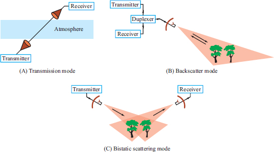
FIGURE 1.1 Active sensing measurement scenarios.
ing System. The receiver may be stationary and located at a coastline or may be onboard an orbiting satellite.
Similarly, astronomical observations may be performed either monostatically or bistatically (see Figure 1.3). A feature common to all active sensing systems is the use of an artificially generated signal radiated by a transmit antenna. This is in contrast to passive sensing, wherein the medium under observation is itself the transmission or emission source; a passive sensor consists of only a receiver configured to measure the naturally generated thermal radiation from the observed medium or reflected radiation from other sources.
The electromagnetic spectrum (Figure 1.4) spans many decades in frequency (or wavelength), with the radio part constituting the frequency range from near 0 Hz to 300 GHz. Some of the applications of the radio spectrum—including communication, navigation, broadcasting, radar, and passive remote sensing—are summarized in Figure 1.5. The radio spectrum is divided into 11 individual bands, the three highest of which (UHF, SHF, and EHF) comprise the microwave band extending between 0.3 GHz and 300 GHz (or, equivalently, between 1 m and 1 mm in wavelength).
The top part of Figure 1.4 provides a spectral plot of atmospheric opacity
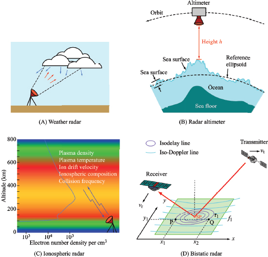
FIGURE 1.2 Active sensing measurement scenarios relevant to Earth remote sensing. SOURCE: (B) and (D) Fawwaz T. Ulaby and David G. Long, Microwave Radar and Radiometric Remote Sensing, University of Michigan Press, Ann Arbor, Mich., 2014. With permission of the authors. (A) and (C) generated by the committee.
under clear-sky conditions. Transmission between Earth’s surface and outer space is limited to frequencies within the electromagnetic atmospheric windows in the visible, infrared, and radio regions of the spectrum. Among these windows, only the radio window allows successful transmission through the atmosphere under cloud-cover conditions.
Atmospheric transmissivity is the inverse of atmospheric opacity. The plot shown in Figure 1.6 displays atmospheric transmissivity as a function of electro-
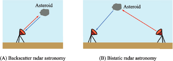
FIGURE 1.3 Radar astronomy uses backscatter and bistatic scattering measurements to extract complementary information about extraterrestrial targets.
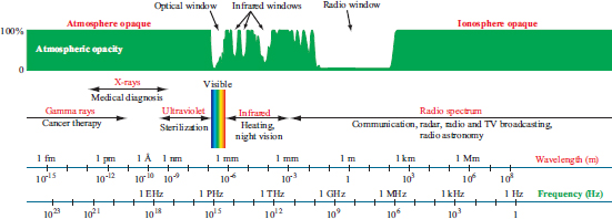
FIGURE 1.4 The electromagnetic spectrum. Atmospheric opacity for Earth is shown along the top. SOURCE: Fawwaz T. Ulaby and David G. Long, Microwave Radar and Radiometric Remote Sensing, University of Michigan Press, Ann Arbor, Mich., 2014. With permission of the authors.
magnetic frequency for the microwave band (300 MHz-300 GHz). The ionosphere is opaque to the transmission of electromagnetic waves at all frequencies below about 15 MHz, depending on ionospheric conditions. Atmospheric transmissivity plays a key role in frequency selection for both active and passive sensing within or through the atmosphere. For example, because of water-vapor absorption near 22 and 183 GHz and oxygen absorption near 58 and 119 GHz, these frequencies are used almost exclusively for passive sensing observations of the atmosphere. In contrast, because at frequencies between about 300 MHz and 20 GHz the atmo-
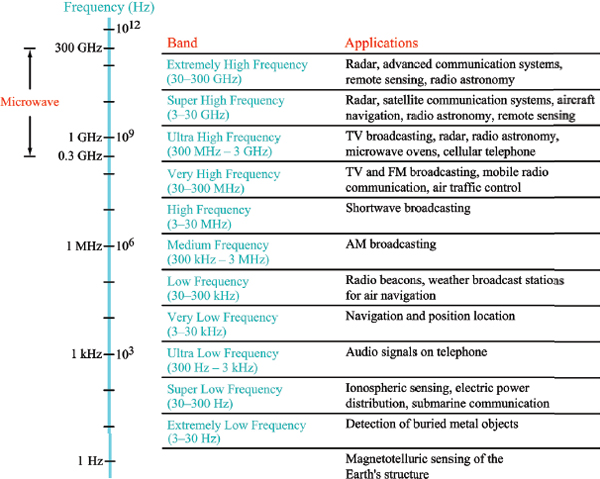
FIGURE 1.5 The radio spectrum and some of its applications. SOURCE: Fawwaz T. Ulaby and David G. Long, Microwave Radar and Radiometric Remote Sensing, University of Michigan Press, Ann Arbor, Mich., 2014. With permission of the authors.
sphere is essentially transparent and signal attenuation is tolerable in atmospheric “windows,” sensors observing Earth’s surface through the atmosphere are operated either at frequencies below 20 GHz or at those within the transmission windows shown in Figure 1.6. Short-range radar applications such as vehicle anticollision radars operate at 77 GHz, where atmospheric attenuation helps minimize interference from distant radars.
Several letter-designation schemes are in common use for sub-bands within
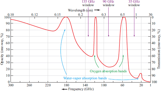
FIGURE 1.6 Percentage transmission through Earth’s atmosphere, along the vertical direction, under clear sky conditions. SOURCE: Fawwaz T. Ulaby and David G. Long, Microwave Radar and Radiometric Remote Sensing, University of Michigan Press, Ann Arbor, Mich., 2014. With permission of the authors.
and adjacent to the microwave band. Two such schemes are described in Table 1.1. The first, an unofficial set used extensively by the microwave remote-sensing community, starts with the P-band (0.225-0.39 GHz) and concludes with the W-band (56-100 GHz). The second set, officially known as the IEEE radar bands, covers the spectral range from 1 GHz to 110 GHz. Because many sensor systems are organized by letter sub-band, it is impractical to entirely exclude the use of such designations in this report. To avoid confusion, however, the associated frequency or frequency interval is always included explicitly.
SCIENTIFIC APPLICATIONS AND SOCIETAL BENEFITS
Chapters 2-4 provide overviews of how active sensing systems are used to extract information about the state of Earth’s atmosphere and its ocean and land surfaces. Separate chapters provide similar information on ionospheric sensing (Chapter 5) and radar astronomy (Chapter 6). A summary of the physical parameters measureable by active sensing is available in Box 1.1. The associated applica-
TABLE 1.1 Common Band Designations
|
|
||
| Band | Remote-Sensing Community Frequency Range | IEEE Radar Frequency Range |
|
|
||
| HF | 3-30 MHz | 3-30 MHz |
| VHF | 30-300 MHz | 30-300 MHz |
| UHF | 0.3-3 GHz | 0.3-3 GHz |
| P | 0.225-0.39 GHz | — |
| L | 0.39-1.55 GHz | 1-2 GHz |
| S | 1.55-4.2 GHz | 2-4 GHz |
| C | 4.2-5.75 GHz | 4-8 GHz |
| X | 5.75-10.9 GHz | 8-12 GHz |
| Ku | 10.9-22 GHz | 12-18 GHz |
| K | — | 18-27 GHz |
| Ka | 22-36 GHz | 27-40 GHz |
| Q | 36-46 GHz | — |
| V | 46-56 GHz | 40-75 GHz |
| W | 56-100 GHz | 75-110 GHz |
|
|
||
NOTE: HF, high frequency; IEEE, Institute of Electrical and Electronics Engineers; UHF, ultrahigh frequency; VHF, very high frequency.
tions extend from the purely scientific, such as the study of the interior structure of planets, to the applications that are essential for health, safety, and commerce.
The radio spectrum is used by many types of services, from radio and TV broadcasting to wireless phone communication; weather, military, and remote sensing radars; and radio and radar astronomy, among many others. The services concerned with scientific uses of the spectrum are listed in Table 1.2. Active sensing, the subject of the present study, encompasses the following:
- Radar remote sensing operates under the Earth Exploration Satellite Service (EESS/active).
- Radar astronomy operates under the Radiolocation Service.
- Weather radar operates under the Radiolocation Service.
- Ionospheric sounding operates under the Meteorological Aids Service.
Regulatory Allocation Process
As discussed in detail in Chapter 7, radio regulations and frequency allocations are developed at both national and international levels. At the international level, regulations are formulated by the Radiocommunication Sector of the International Telecommunications Union (ITU-R). The process is described in some detail in
BOX 1.1
Selected Applications of Active Sensing Systems
Radar Remote Sensing
Geology—tectonics, seismology, volcanism, geodesy, structure, lithology.
Hydrology—soil moisture, watershed mapping, flood mapping, mapping of surface water (ponds, lakes, rivers), snow mapping.
Agriculture—crop mapping, agricultural-practice monitoring, identifying field boundaries, monitoring growth and harvest progress, identifying stress areas, rangeland monitoring, water problems—same as hydrology.
Forests—monitoring cutting, mapping fire damage, identifying stress areas, vegetation density, and biomass.
Cartography—topographic mapping, land-use mapping, monitoring land-use changes, urban development.
Polar regions (cryosphere)—monitoring and mapping sea ice, detecting and tracking icebergs, mapping glacial ice sheets, monitoring glacial changes, including measuring velocity.
Ocean—measuring wave spectra, monitoring oil spills, monitoring ship traffic and fishing fleets, wind speed and direction measurement, rain, clouds, measuring currents, undersea mapping.
Weather Radar
Quantitative precipitation estimation (aka rainfall estimation), flash flood warnings, severe storm warnings, forensic meteorology for the insurance industry, risk mitigation, aviation/transportation safety—wind shear detection, television weather forecasts, mesoscale meteorology, numerical weather prediction via data assimilation, urban meteorology.
Ionospheric Sounding
Ionospheric plasma density structure, plasma dynamics, upper atmospheric heating, storms and substorms, radio propagation, ground-satellite communication impacts, radiation belt impacts on spacecraft, GPS disruptions, ground-induced currents in pipelines and power systems.
Astronomy
Precision orbits for impact assessment and mitigation of potentially hazardous near-Earth asteroids, surface and interior properties of near-Earth asteroids, interior structure of planets and satellites, support for space missions, evolution of the solar system, surface properties of the terrestrial planets and the Moon.
the National Research Council Handbook of Frequency Allocation and Spectrum Protection for Scientific Uses.1
______________
1 National Research Council, Handbook of Frequency Allocation and Spectrum Protection for Scientific Uses, The National Academies Press, Washington, D.C., 2007.
TABLE 1.2 Science Services
|
|
||
| Service | Abbreviation | Description of Service |
|
|
||
| Active Sensing Services | ||
|
Earth Exploration—Satellite Service |
EESS | Remote sensing from orbit, both active and passive, and the data downlinks from these satellites |
|
Meteorological Satellite Service |
MetSat | Weather satellites |
|
Radiolocation Service |
RLS | Radar astronomy, weather radar |
| Support Services | ||
|
International Global Navigation Satellite System (GNSS) Service |
IGS | Accurate position and timing data |
|
Meteorological Aids Service |
MetAids | Radio communications for meteorology, e.g., weather balloons, ionospheric sounding |
|
Space Operations Service |
SOS | Radio communications concerned exclusively with the operation of spacecraft—in particular, space tracking, space telemetry, and space telecommand |
|
Space Research Service |
SRS | Science satellite telemetry and data downlinks, space-based radio astronomy, and other services |
|
|
||
The aforementioned handbook describes the frequency allocation process within the United States as follows:
Non-federal-government use of the spectrum is regulated by the Federal Communications Commission (FCC). Federal government use is regulated by the National Telecommunications and Information Administration (NTIA), which is part of the U.S. Department of Commerce. Most, if not all, spectrum use for scientific research is under shared federal government/non-federal-government jurisdiction. Many federal agencies have spectrum-management offices—for example, the Department of Defense (DOD), National Aeronautics and Space Administration (NASA), and the National Science Foundation (NSF). The Interdepartment Radio Advisory Committee (IRAC) is a standing committee that advises NTIA with respect to the spectrum needs and use by departments and agencies of the U.S. government.
The U.S. administration has set up national-level study groups, working parties, and task groups that mirror those that operate within the ITU-R. For example, U.S. Working Party 7C (U.S. WP7C), part of U.S. Study Group 7, develops U.S. positions and draft documents concerning remote sensing. These documents are reviewed by the United States International Telecommunication Advisory Committee (ITAC) and, if approved, are forwarded by the U.S. Department of State to the ITU-R as input for international meetings.
TABLE 1.3 EESS (Active) Frequency Allocations
| Band Designation | Frequency Band as Allocated in Article 5 of the Radio Regulations | Application Bandwidths | ||||
| Scatterometer | Altimeter | Imager | Precipitation Radar | Cloud Profile Radar | ||
| P-band | 432-438 MHz | 6 MHz | ||||
| L-band | 1,215-1,300 MHz | 5-500 kHz | 20-85 MHz | |||
| S-band | 3,100-3,300 MHz | 200 MHz | 20-200 MHz | |||
| C-band | 5,250-5,570 MHz | 5-500 kHz | 320 MHz | 20-320 MHz | ||
| X-band | 8,550-8,650 MHz | 5-500 kHz | 100 MHz | 20-100 MHz | ||
| X-band | 9,300-9,900 MHz | 5-500 kHz | 300 MHz | 20-600 MHz | ||
| Ku-band | 13.25-13.75 GHz | 5-500 kHz | 500 MHz | 0.6-14 MHz | ||
| Ku-band | 17.2-17.3 GHz | 5-500 kHz | 0.6-14 MHz | |||
| K-band | 24.05-24.25 GHz | 0.6-14 MHz | ||||
| Ka-band | 35.5-36 GHz | 5-500 kHz | 500 MHz | 0.6-14 MHz | ||
| W-band | 78-79 GHz | 0.3-10 MHz | ||||
| W-band | 94-94.1 GHz | 0.3-10 MHz | ||||
| mm-band | 133.5-134 GHz | 0.3-10 MHz | ||||
| mm-band | 237.9-238 GHz | 0.3-10 MHz | ||||
Table 1.3 lists frequency bands and associated bandwidths used for spaceborne active sensors operating in the EESS, per Recommendation ITU-R RS.577-7 of the ITU. Contained in the overall list are the bands commonly used for each of the five types of active sensors on satellite platforms—namely, scatterometers, altimeters, imagers, precipitation radars, and cloud profiling radars. More detail about individual bands is available in Appendix C.
Radars used for astronomical observations use bands allocated to the Radiolocation Service. Table 1.4 lists bands used by current systems as well as those associated with potential new planetary radar systems under consideration for the future. The bands commonly used for radar ionospheric studies are listed in Table 1.5.
Scientific Basis for Frequency Choices
The choice of frequency, or combination of multiple frequencies, for sensing a particular physical parameter in Box 1.1 is dictated by three factors:
- The transmission spectrum of the medium between the radar and the target of interest. As noted earlier in connection with Figure 1.6, the atmosphere is essentially transparent to electromagnetic wave propagation at frequencies between 100 MHz and 20 GHz and partially transparent within the
TABLE 1.4 Radar Astronomy Frequency Bands
| Transmitting Location | Frequency (GHz) | Bandwidth (MHz) | Power | Receive Location |
| A. Current Planetary Radar Systems | ||||
| Arecibo, Puerto Rico | 2.380 | 20 | 1.0 MW average | Arecibo, Puerto Rico GBT, Green Bank, West Virginia VLA, Socorro, New Mexico LRO, Lunar orbit |
| 0.430 | 0.6 | 2.5 MW peak, 150 kW average | Arecibo, Puerto Rico GBT, Green Bank, West Virginia | |
| Goldstone, California, DSS-13 | 7.190 | 80 | 80 kW average | Goldstone, California GBT, Green Bank, West Virginia Arecibo, Puerto Rico |
| Goldstone, California, DSS-14 | 8.560 | 50 | 500 kW average | Goldstone, California GBT, Green Bank, West Virginia Arecibo, Puerto Rico VLA, Socorro, New Mexico 10 VLBA sites |
| B. Potential New Planetary Radar Systems | ||||
| GBT, Green Bank, West Virginia | 8.6 | 100 | 500 kW average | GBT, Green Bank, West Virginia VLA, Socorro, New Mexico Goldstone, California |
| Arecibo, Puerto Rico | 4.6 | 50 | 500 kW average | Arecibo, Puerto Rico GBT, Green Bank, West Virginia |
| Goldstone, California, DSS-14 | 8.60 | 120 | 1.0 MW average | Goldstone, California GBT, Green Bank, West Virginia Arecibo, Puerto Rico |
NOTE: Close asteroid observations require bistatic operation. GBT, Green Bank Telescope; LRO, Lunar Reconnaissance Orbiter; VLA, Very Large Array; VLBA, Very Long Baseline Array.
-
transmission windows centered at 35, 90, and 135 GHz. Hence, microwave satellite sensors used to observe Earth’s surface are limited to frequencies within these bands. The specific choice of frequency within an atmospheric transmission window is usually dictated by factor (b), namely the physical mechanism responsible for the process that is remotely observed.
- Scattering mechanism. Water droplets in a nonprecipitating cloud are much smaller than those in rain. Consequently, different frequencies are best suited for measuring the water content of a water cloud as opposed to the rainfall rate of a precipitating cloud. In the frequency allocations list of Table 1.3, the frequencies associated with precipitation radar extend between 13.25 GHz and 36 GHz, whereas those associated with cloud profiles extend between 78 GHz and 238 GHz.
TABLE 1.5 Ionospheric Radar Frequency Bands
| Radar | Location | Frequency/Bandwidth | Power | License |
| SuperDARN | Global | 8-20 MHz instantaneous BW 60 kHz | 10 kW | Within the United States—FCC experimental noninterference |
| Digisonde | Global | 2-30 MHz | 500 W | |
| Arecibo ISR | Arecibo, Puerto Rico | 430 MHz, 500 kHz BW | 2.5 MW | NTIA |
| Millstone Hill ISR | Westford, Massachusetts | 440.0, 440.2, 440.4 MHz, 1.7 MHz BW | 2.5 MW | NTIA noninterference |
| PFISR | Poker Flat, Alaska | 449.5 MHz, 1 MHz BW | 2 MW | NTIA Primary |
| RISR | Resolute Bay, Nunavut, Canada | 442.9 MHz, 4 MHz BW | 2 MW | Industry Canada |
| Sondrestron | Kangerlussuaq, Greenland | 1287-1293 MHz, 1 MHz BW | 3.5 MW | |
| Homer VHF | Homer, Alaska | 29.795 MHz, 100 kHz BW | 15 kW | FCC experimental noninterference |
| Jicamarca ISR | Jicamarca, Peru | 49.92 MHz, 1 MHz BW | 6 MW | Peruvian |
| HAARP | Gakona, Arkansas | 2.6-9.995 MHz instantaneous BW 200 kHz | 3.6 MW CW | NTIA |
NOTE: BW, bandwidth; CW, continuous wave; FCC, Federal Communications Commission; HAARP, High Frequency Active Auroral Research Program; ISR, Ionosondes and Incoherent-Scatter Radar; NTIA, National Telecommunications and Information Administration; PFISR, Poker Flat, Alaska, Incoherent-Scatter Radar; RISR, Resolute Incoherent Scatter Radar; VHF, very high frequency.
-
Similar arguments apply to the choice of frequencies for radar measurements of other physical parameters (Figure 1.7). From a radar perspective, a vegetation canopy is a “cloud” of branches and leaves whose sizes and dielectric properties dictate the nature of the scattering within the vegetation volume, and consequently, the optimum choice of frequencies for measuring biomass or for penetrating the canopy to sense the moisture content of the soil surface beneath it. Ocean scattering depends on the spatial spectrum of waves on the ocean surface relative to λ. Radar scattering by the ionosphere is strongly dependent on the plasma density, the strength of the ambient magnetic field, and the frequency and polarization direction of the incident radar wave. In radar astronomy, the degree of scattering by the surface of a planet or satellite is related to the scale of roughness of the surface relative to λ.
- Hardware, cost, and operational constraints. The cost and feasibility of a radar design often are constrained by two critical system parameters: the operating
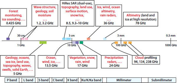
FIGURE 1.7 The choice of frequencies for satellite active sensing is dictated by the physics of the relevant scattering mechanism.
frequency and the average transmit power. Increasing the frequency from 10 GHz, for example, to 100 GHz (while keeping antenna size and all other specifications the same), leads to a substantial increase in cost because transmitter and receiver technology is much better developed at 10 GHz than at 100 GHz. By the same token, because of technology improvements over the past two decades, some systems that were considered unfeasible for satellite operation in the 1990s are now under consideration for future missions.
Transmitter power is a critically important factor for radar astronomy. Because of the long distance between Earth-based radars and their intended targets, it is necessary to transmit signals with powers on the order of megawatts, which requires the use of special types of klystrons. Advances in klystron technology leading to successful operation at higher frequencies and/or higher power has led to proposed upgrades of current radar astronomy facilities as noted in Table 1.4. Higher average power allows for wider bandwidths, which provide for better spatial resolution.
RADIO-FREQUENCY INTERFERENCE AND MITIGATION OPPORTUNITIES
Radio-frequency interference (RFI) refers to the unintended reception of a signal transmitted by an auxiliary source. Active sensors use transmitters and receivers,
so an active sensor may act as the source of interference to a communication system, a passive sensing system, or another radar system, or the receiver of the active sensor may be the recipient of an unintended signal radiated by an external source. Chapter 8 provides a review of the available information on documented occurrences of RFI, organized by frequency band, starting with the HF band (3-30 MHz) and concluding with the W-band (56-100 GHz). One of the conclusions deduced from the review is that while there is evidence that RFI occurs fairly frequently at the C-band and lower frequencies, its occurrence is rare at higher frequencies. Moreover, the preliminary evidence suggests that active sensing instruments do not normally cause RFI to other users but that other users have negatively impacted the performance of active sensing instruments.
Another topic alluded to in Chapter 8 is RFI mitigation and the degree to which mitigation techniques have been applied successfully. This is followed in Chapter 9 with a detailed examination of the various tools available for avoiding or mitigating RFI, and the limitations thereof.


