
Overall Assessment of CAFE Program Methodology and Design
The reformed Corporate Average Fuel Economy (CAFE) standards adopted into final regulations in 2010 for model year (MY) 2012-2016 vehicles and then in 2012 for MY 2017-2021 are quite different from the earlier CAFE standards in a number of important ways. The most significant changes have been mentioned already in this report and include harmonizing the fuel economy and greenhouse gas (GHG) standards and increasing the stringency of the standards in each successive year from MY 2012 to MY 2021. The GHG standards are final to 2025, and the CAFE standards are final to 2021 and “augural” for MY 2022 to 2025.1 Standards had to be set in each year at “maximum feasible” levels through 2030, considering “technological feasibility, economic practicability, the effect of other motor vehicle standards of the Government on fuel economy, and the need of the United States to conserve energy” (49 U.S.C. 32902 (f)). This chapter discusses the legislative mandates calling for standards, their enforcement via test cycles, design of the standards and possible societal costs and benefits. Key design changes for the 2017-2025 CAFE and GHG standards are highlighted. Regulation of fuel economy by vehicle footprint and credit banking and trading, as well as by the special provisions for alternative technology vehicles (ATVs) and alternative fuel vehicles (AFVs) are all discussed.
CHOICE OF VEHICLE ATTRIBUTES IN THE DESIGN OF CURRENT REGULATIONS
The Energy Independence and Security Act (EISA) legislation in 2007 required that new fuel economy standards be based on vehicle attributes—that is, they would vary in some way by vehicle mass, size, or other relevant characteristics. The relevant fuel economy or GHG target for a vehicle would be calculated based on a mathematical formula that related the attribute to the target. The attribute-based standards began in MY 2009 for light trucks2 and MY 2012 for passenger cars. Compliance with the standards is assessed at the manufacturer level, so a sales-weighted average of a manufacturer’s fleet must meet the sales-weighted attributed-based standard. Vehicle footprint, determined by multiplying the vehicle’s wheelbase by the vehicle’s average track width, was chosen as the attribute upon which to base the standards (EPA/NHTSA 2012a, 62639). The National Highway Traffic Safety Administration (NHTSA), the Environmental Protection Agency (EPA), and others argue that the footprint standard encourages more technology for improved fuel economy across all vehicle sizes, with less incentive to either upweight, as could be the case with a mass-based standard, or to downsize if the standard was the same for all vehicles. In fact, NHTSA appears to be most concerned with the potential safety implications of downsizing. The issue of how the standards and vehicle safety interact is complex and is discussed in more detail below.
Several possible attributes were considered in setting the standards before the footprint standard was chosen. European, Japanese, and Chinese standards depend on vehicle weight, with heavier vehicles allowed to have more lenient standards. However, one argument for the footprint standard over the weight standard is that the former would provide incentives for manufacturers to improve fuel economy by weight reduction, rather than size reduction, thus mitigating any adverse safety impacts. A weight-based standard would not provide the same incentive, since lighter vehicles would face a tighter standard (German and Lutsey 2010). There is also concern that weight-based standards may incentivize manufacturers to make vehicles heavier, to reach a lower standard, thereby undermining some of the fuel sav-
_____________
1 NHSTA describes the “augural” MYs 2022-2025 standards as not final and “as representative of what levels of stringency the agency currently believes would be appropriate in those model years, based on the information before us today.”
2 CAFE standards for light trucks for MY 2008-2011 included a reform to the structure for CAFE standards for light trucks and gave manufacturers the option for MY 2008-2010 to comply with the reformed standard or to comply with the unreformed standard. The reformed standard was based on the vehicle footprint. The unreformed standard for 2008 was set to be 22.5 mpg.
ings and CO2 emissions reductions. A recent study by Ito and Sallee (2013) of the weight-based regulations in Japan suggests that vehicle weight may have increased as a result of the standards there.
Relative to a weight-based standard, incentives to increase vehicle size under a footprint standard are less clear because some argue that moving to a larger footprint requires a significant redesign of the vehicle (German and Lutsey 2010). Incentives to increase size are still theoretically possible and will depend on the cost of meeting the standard for vehicles of different sizes and consumer willingness to pay higher prices for vehicles of different sizes.
A strong motivation for a footprint-based standard is that its cost tends to fall more evenly on all manufacturers, allowing the domestic companies who produce a larger-sized fleet to meet a less-stringent fleetwide average standard than, for example, the Asian companies. The Asian manufacturers tend to advocate a more uniform standard since they build smaller, lighter vehicles. However, the footprint standard does not give any advantages to the European manufacturers, who tend to build vehicles with higher horsepower for their size.
The committee turns next to more discussion of the effects of the footprint standards on vehicle size mix and on vehicle safety. Vehicle safety from a mass reduction standpoint is also discussed in Chapter 6.
Effects of the Footprint Standard on Vehicle Size and Size Mix in the Fleet
There is some concern that the footprint standard may create the unintended incentive for manufacturers to increase the size of any given vehicle so as to lower the applicable standard. As discussed above, many argue that this type of perverse incentive is less likely compared to a weight-based standard, but it may still be an issue and should be carefully considered. In fact, the earlier CAFE standards were also attribute-based—vehicle class in that case—with one standard for passenger cars and a less stringent one for light trucks. The lower standard for trucks may have helped to accelerate the dramatic growth in CUVs, SUVs, and minivans (most of which are classified as light trucks) in the late 1980s and 1990s, when light truck sales went from 20 percent of the light-duty fleet in 1980 to over 50 percent of the fleet in 2000. The less stringent standard for light trucks was not the only reason for this change, but some of the class shifting that occurred may have been an unintended consequence of the regulations.
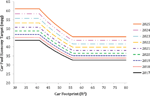
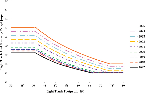
The footprint curves for cars and trucks in MY 2017-2025 are shown in Figure 10.1. The curves indicate the standard a vehicle of a given footprint must meet, with a new, more stringent curve for each model year. There is one set of curves for cars and another for light trucks, with the light truck curve being less stringent for any given footprint and also with a different slope and cutpoints than for cars.
The Agencies carried out extensive analyses about how to set the slope and cutpoints of the car and truck footprint curves. To try to prevent incentives to shift the size of vehicles, the Agencies developed an empirical relationship between footprint and fuel use based on sales-weighted 2008 fuel economy and footprint data, and used this relationship to set the slope of the curve. This is a reasonable attempt to reflect a general trade-off between footprint and energy use, but it does not ensure that there are no incentives to upsize or downsize created by the regulations. The incentives will depend, for example, on the costs of increasing a vehicle’s footprint compared to the savings in meeting a lower fuel economy level. This will differ across vehicles. It will also depend on the profitability of vehicles of different sizes and the ability to pass higher costs on in the marketplace (elasticities of demand for vehicles of different sizes and types).
Possible Outcomes of a Footprint-Based Standard
Three outcomes related to the size of vehicles in the fleet are possible due to the regulations: Manufacturers could change the size of individual vehicles, they could change the mix of vehicle sizes in their portfolio (i.e., more large cars relative to small cars), or they could change the mix of cars and light trucks. The questions are these: What, if any, incentives are created by the footprint standard? How important are the resulting sales outcomes for the goals of the policy, including safety, fuel consumption, and GHG emissions?
The current assumptions in the societal cost-benefit analysis of the rule are that there will be no change in vehicle size or in vehicle size mix from the reference case (no regulation) as a result of the regulation. However, size mix is assumed to change to a slightly smaller vehicle fleet between 2017 and 2025, regardless of the regulation (EIA 2014).
Shifts in the Car/Light Truck Mix
Separate car and light-truck standards might incentivize a shift to light trucks from cars. The light truck standards are less strict and do not rise with size as fast for light trucks as they do for cars. This is especially true for large light trucks. The Agencies give a number of reasons why this is the case, including the fact that many large trucks tend to have low weight relative to their size (e.g., flat beds in pickups) and have greater need for towing capabilities. Several auto companies argued that the standards favor companies with a relatively large number of trucks in their fleets, implying there may be incentives to make larger, less fuel-efficient vehicles. However, factors such as added weight and four-wheel drive (as opposed to two-wheel drive) make it more expensive to shift a vehicle from a car to a truck, by definition. The committee heard arguments that there should be a single footprint curve for all vehicles instead of separate ones for cars and for trucks. As the standards become more stringent each year,
relative costs may also change over time. In the 2017-2025 National Program, credit trading between car and truck fleets will be allowed, as discussed in more detail in this chapter. This creates a new set of incentives, depending on the cost of meeting the rules on the different types of vehicles. For example, if higher fuel economy for trucks is more costly or less profitable than for cars, the manufacturers could comply by exceeding the standards for cars, while being below the standard for trucks.
Changes in Vehicle Model Footprint
Individual vehicle footprints could also change over time. The footprint of a specific vehicle model could be increased because the cost is less than the higher cost of compliance with the standard at the lower footprint, or decreased if cost savings are greater if size is reduced. Alternatively, a specific vehicle model configuration could be dropped and another adopted because of incentives created by the rules. NHTSA and EPA have considered the issue of size shifting in setting the footprint standard and in the Regulatory Impact Assessment (RIA). The EPA RIA references the study by Whitefoot and Skerlos (2011), which uses an economic–engineering model of the vehicle fleet and changes in the fleet over time and finds that there could be some increase in vehicle size overall as a result of the footprint-based regulations, based on data available at the time of the study. As a first approach to determining if there are particular trends emerging as a result of the rules, changes in such vehicle nameplates and footprints can be monitored over time, although it is difficult to distinguish between changes occurring in the fleet due to the rule versus those that are occurring for other reasons.
Changes in Vehicle Fleet Mix
An economic behavioral model would be useful for predicting the effects of the standards on the fleet. For example, as the fuel economy standards are made more stringent over time, what is the relative shift in the marginal costs for vehicles of different sizes and how would those changes affect purchase decisions across the fleet? Are the proportionate changes in small car costs greater than large car costs, as might be expected? What is known about the elasticities of demand for vehicles of different sizes and market segments? This last question is relevant for predicting how difficult it will be to pass costs forward in different model segments. There are some estimates from the industry and from the economics literature on elasticities, but it is unclear how reliable these are. Estimates tend to show that the vehicle size/types with the lowest own-price elasticities of demand are for both large and small SUVs and large pickup trucks. If the costs of compliance are relatively lower for larger vehicles and these costs can more readily be passed on in the form of higher prices, then there could be some shift toward larger vehicles. An estimate of these impacts could help assess whether the standards create incentives that adversely affect fuel consumption, safety, and environmental outcomes.
Some recent papers have tried to incorporate these effects into models that integrate the engineering data with economic behavior of manufacturers and consumers over time. These models are potentially useful for looking at the full effects of the regulations over time, including producer and consumer responses to costs and price changes in different vehicle segments. They can also provide insight about the full costs and benefits of the regulations. The Whitefoot and Skerlos (2011) analysis is one such model, and there have been others, including one by Jacobsen (2013a) and one by Gramlich (2010). All of these models find some tendency for the size of the fleet to increase with the current footprint standards, with larger effects in the market for trucks. In particular, because of the shape of the footprint curves, the greatest incentives are for small and medium-sized trucks to get larger. Vehicle mix may also be affected by shifts from the light-duty to the medium-duty market, such as from Class 2a trucks to Class 2b trucks if the trade-off in costs is favorable. Another potential effect of the rule is to influence old vehicle scrappage rates as the price of both new and used vehicles changes over time (e.g., Jacobsen and van Benthem 2015). More attention to issues related to the overall effect of the regulations on the fleet composition is warranted. Discussion of the impact of the standards on vehicle size mix from a consumer perspective can be found in Chapter 9. The mix of vehicles needs to be tracked over time, as the Agencies are starting to do, but economic models are also important for forecasting how the mix will change.
Effect of the Footprint Standard on Vehicle Safety
The effect of attribute-based standards on vehicle safety is a complex question for a number of reasons. The mass disparity between the vehicles involved in a crash seems to be a key factor in assessing safety, with the risks for those in the lighter vehicle increasing along with the mass of the heavier vehicle (Evans 1991; NHTSA 2012a; LBNL 2012a). This implies that the greater the size disparity in the fleet, the more fatalities there are likely to be. In the past, size and mass have been highly correlated, but that has become less true recently, and the footprint standards will tend to reduce mass while attempting to keep the footprint relatively constant.
Figures 10.2a and 10.2b show the trends in distribution of vehicle weight in the fleet by car and truck from 1975 to 2007. The figures show a good deal of variation in weight for both cars and trucks, with light trucks substantially heavier than cars. Since 1991, there has been a trend toward greater weight for both cars and trucks. This likely reflects in part preferences for larger cars that consumers perceive to be safer. Figures 10.2a and 10.2b also indicate that cars have been getting heavier except for the largest passenger cars, which became much less common between 1975 and 1991, with the shift from cars to trucks. Small trucks (less than
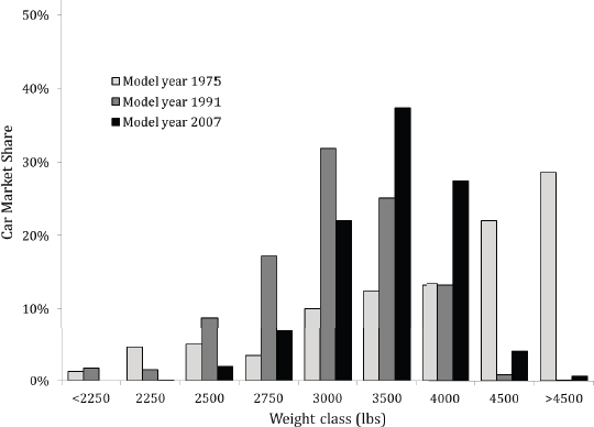
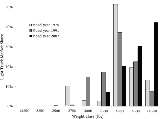
3,000 lb) largely disappeared from the market, and there was a large increase in trucks greater than 4,000 lb between 1991 and 2007.
NHTSA favors the footprint-based standard in part because the Agency is concerned that any CAFE regulation that results in a downsizing of new vehicles will result in more fatalities, at least in the short term, compared to a regulation that tends to add new vehicles with the current footprint size distribution. NHTSA argues that alternative CAFE rules such as a more uniform standard would tend to result in some downsizing. There is concern that downsizing the fleet at this time will have adverse effects on safety. Much of the recent statistical evidence on safety suggests, among other things, that maintaining vehicle footprint while reducing vehicle mass may have better safety outcomes than a policy that reduces both the mass and size of the vehicles in the fleet. These studies, which are summarized in Chapter 6, attempt to isolate the effects of vehicle footprint from mass on fatalities in vehicle crashes. This is a major reason for NHTSA’s implementation of the footprint standard in the recent CAFE revisions.
The Agencies may want to consider the impact on overall fleet mix and associated safety due to individual choices. When some consumers buy larger vehicles because they believe they will afford them more safety in a crash, they are not accounting for the external costs of their decision. These consumers are likely more concerned with their own safety and may not consider the societal impacts of their decision. From a social welfare perspective, this leads to a vehicle fleet that is on average heavier than is optimal and may result in more fatalities (Li 2012) than would a lighter fleet. In one study of vehicle safety, Anderson and Auffhammer (2013) attempt to estimate the magnitude of this accident-related externality and find that it is quite large.
The estimated effects of reducing mass or footprint are small compared to other vehicle attributes, driver characteristics, and crash circumstances (Figures 2.5 to 2.10 of Wenzel 2012). While, on average, mass reduction in lighter-than-average cars is associated with a small increase in fatality risk, there is a large range in risk for cars of the same mass, even after accounting for differences in vehicles, drivers, and crash circumstances (Section 4 of Wenzel 2012). It is important to note that the data used for the statistical analyses rely on historical data from recent vehicle designs and that the mass and size distribution of the fleet, and designs of vehicles, are likely to change by the time the standards become effective in MY 2017 to 2025.
NHTSA argues that alternative CAFE rules such as a more uniform standard would tend to result in some downsizing of the fleet in terms of both size and weight and that this would have an adverse effect on safety. One interesting study from the economics literature finds that this may not be the case, however. Jacobsen (2013a) analyzed different regulatory approaches for CAFE using a model of accidents that accounts for different vehicle size and safety attributes and driver behavior. His analysis suggests one standard or set of standards for vehicles, and not a separate one for cars and trucks. Though there may be some downsizing from this approach, there may also be a shift away from trucks, which makes the fleet more uniform in size. He finds that the changes in these risks offset each other.
In any case, the credit trading discussed later in this chapter should equalize the net marginal cost of fuel economy improvements across all vehicle types and manufacturers, in theory, limiting concerns about multiple standards.
Overall, evidence from available data suggests that the effect of the fuel economy rules on vehicle safety is likely to be relatively small. The selection of footprint as the attribute on which the standards are based provides a reasonable approach to a safety-neutral standard based on the information currently available. However, there should be continued study of the relationship between vehicle size, weight, and safety, and the effects of overall fleet size and mix on societal risk.
An important aspect of the 2017-2025 MY CAFE/GHG standard is flexibility in the means and timing of compliance offered via new opportunities in banking, borrowing, transferring, and trading “credits.” Vehicle manufacturers have always had some flexibility in meeting CAFE standards, such as averaging across models in their fleet, banking credits, and paying civil penalties to comply. In the CAFE/GHG standards, credits can be earned for vehicles that have lower fuel use or GHG emissions than the target for that footprint, and can be used to offset higher fuel use or emissions of vehicles that are above the footprint-based target. Auto manufacturers have additional opportunities to earn credits, such as by producing certain AFVs or implementing technologies with off-cycle benefits (e.g., improved air conditioner efficiency). These technology-based credits are described in this chapter and in Chapter 6. The principle under fully tradable fuel economy and emissions credits is that there is a target total amount of fuel consumption and greenhouse gas emissions reductions over a period of time, but when those reductions occur and which vehicles and companies implement them are flexible. This allows the targets to be met at a lower cost.
The 2017-2025 CAFE/GHG standards allow greater flexibilities for credit trading over time, between car and truck fleets and across manufacturers. Opportunities for a manufacturer to bank and borrow credits over time will allow that manufacturer to better match product redesign cycles that are usually between 3 and 5 years, with the standard increasing in stringency every year. In addition, trading credits across companies can allow cost savings because some companies have a much greater difficulty meeting the standards than others due to differences in product types and range of vehicles offered. This increased flexibility in meeting standards is likely to be important for manufacturer compliance with
the regulations. Credit trading is just beginning under the new rules, and it will be important to assess and possibly revise the provisions of the trading rules over the next few years. A key element of this assessment is whether the credit provisions of the two Agencies allow similar flexibility or whether one set of rules is more binding.
Manufacturer Averaging of Fuel Use and Emissions Across Models in Their Fleet
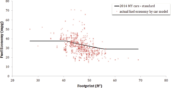
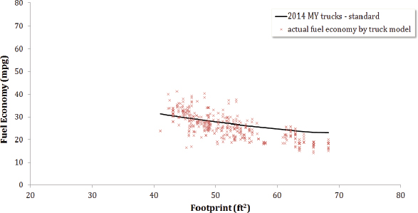
Each manufacturer is in compliance with the national program standards if the footprint-based, sales-weighted fleet average of fuel economy and GHG emissions is at least equivalent to the fleet-average, footprint-based standard given the actual size mix of vehicle sizes sold by the firm. A manufacturer faces two standards under both the CAFE and GHG regulations, one for cars and a more lenient one for trucks.3 Manufacturers can average fuel consumption or emissions across all vehicles in a class (cars or light trucks), allowing substantial variation in individual model emissions and fuel consumption, even for vehicles of the same footprint. Figures 10.3 and 10.4 show the variation in fuel consumption by footprint across the entire fleet for cars and for trucks. Figure 10.3 shows the actual fuel economy for each of about 1,100 car makes and models (in red) relative to the fuel economy standard of each car based on its footprint for model year 2014. Certification fuel economy vs. vehicle footprint data for each manufacturer also shows a range of actual fuel economies relative to the standards for individual vehicle manufacturer car fleets (not shown). Figure 10.4 shows footprint and fuel economy for all trucks for the 2014 model year along with the truck standard in 2014.
It is clear from these graphs that there are a range of vehicles on the market with different fuel economies and other characteristics, even with similar footprints. Averaging within the vehicle classes (and across vehicle types and manufacturers, as we discuss below) allows manufacturers to offer a range of vehicle types and characteristics, including fuel economy. Consumers will continue to have choices about fuel economy relative to other characteristics, so the issue of how they value fuel economy remains critically important to the impact of the standards.
Defining Fuel Economy and GHG Credits
Both NHTSA and EPA allow companies to use credit surpluses or deficits in meeting the standards, but the two Agencies define credits differently, due to different regulatory mandates. This may have important consequences for automakers in meeting both standards. Because the 2017-2025 standards depend on the footprint of each vehicle, under both rules, the relevant car and light truck standards for each manufacturer will be different from those of other manufacturers and will depend on the mix of sizes of vehicles the firm sells. For EPA, the greenhouse gas standards are in terms of grams of CO2 equivalent per mile, or in total grams of CO2 equivalent over the lifetime of the vehicle. A manufacturer earns credits when it produces vehicles with less CO2 per mile than its production-weighted footprint standard. Deficits are the opposite—they occur when the manufacturer’s actual fleet GHG emissions exceed its production-weighted footprint standard. Credits or deficits are converted into total grams of CO2 under or over the standard over the life of the vehicles, using an estimated car or truck lifetime vehicle miles traveled (VMT). Cars and trucks are assumed to have different lifetime VMTs, estimated by NHTSA at 195,264 miles for passenger cars and 225,865 miles for light trucks.
Under CAFE rules, a manufacturer earns credits when the vehicles it produces use less fuel per mile than the production-weighted footprint standard requires and faces credit deficits when it produces vehicles that on average have fuel use greater than the standard. A credit or deficit is earned for each 0.1 mpg difference between the standard and the actual mpg for each vehicle. Total credits earned by a manufacturer are the sum of these differences across all vehicles produced in a given year. Credits must be traded in terms of fuel consumption rather than fuel economy and so are adjusted for a vehicle’s fuel consumption over the life of the vehicle.
The ability of manufacturers to earn credits is also impacted by other provisions of the NHTSA and EPA rule. For example, in the EPA program, credits are earned for the production of alternative fuel vehicles, for off-cycle emissions reductions, and for air conditioning adjustments. Many of these additional ways of earning credits are described in detail in Chapter 6. The following sections address how credits may be traded, the role they have in compliance, and whether robust markets in credits are likely to develop.
Transferring Credits Between Cars and Trucks
One new provision of the rules that went into effect starting in model year 2012 is that each manufacturer can trade credits between its own car and light truck lines for both fuel use and GHG emissions. This is referred to by the Agencies as transferring credits. So, for example, if a manufacturer’s light truck fleet does not meet the light truck standard, that manufacturer can overcomply on the cars it produces and transfer the credits to the light truck fleet to make up the shortfall.
The preliminary evidence is that in the first few years of the EPA GHG program, 2012 and 2013, most of the auto companies earned many more GHG emissions credits for cars than they earned for trucks (EPA 2014a). In addition, in
_____________
3 Since the inception of the CAFE standards, manufacturers have been allowed to average fuel economy across models within their own car and light truck fleets. An exception to this is that each manufacturer must meet a specific minimal standard for domestically produced vehicles. The domestically produced standard cannot be met with more efficient imported vehicles.
reporting to the EPA, about half of the roughly 20 manufacturers reported earning credits for overcompliance of their car fleets, and the other half were in deficit due to under-compliance. For trucks, only three of the companies earned credits in 2012, and overall, the industry was in a deficit with respect to the truck standards (EPA 2014a, 16). The data are not yet available from NHTSA on credits earned by cars and trucks by manufacturer, but it is likely to be similar.
This suggests that it may be more costly for manufacturers to comply with the early standards by reducing fuel use or emissions from light trucks than cars. The issue also appears to be driven by the fact that the large car market shrunk during the 1990s and was replaced by SUVs and CUVs classified as light trucks, making it easier for manufacturers to meet their car standards. It must be noted that some of the manufacturers reporting deficits in their light truck fleets used previously accumulated credits from earlier years to offset those deficits. Because credits can be banked and used in later years, drawing conclusions for any one year is difficult. It will be interesting to see if the tendency for lower compliance on the truck side persists.
Allowing manufacturers to transfer credits between its car and truck fleets will allow the automakers to meet the standards in the most profitable and cost-effective ways.
This flexibility will become increasingly important as the standards become stricter over time.
Banking Credits
Both NHTSA and EPA allow credits to be traded backward and forward over time, called banking. They allow firms to carry credits up to 5 years into the future and back in time for up to 3 years. For example, if a company cannot comply with its average standard for cars this year, it can borrow forward from its future fleets in one or more of the next 3 years, effectively making the standards they must meet more stringent in at least one of those years.
In a system with banking of credits, it is important to determine when to allow the companies to start banking. Both EPA and NHTSA allowed companies to bank credits for 3 years before the first year of the new rules (NHTSA has always allowed banking). This means companies were allowed to bank in 2009, 2010, and 2011. Not all companies overcomplied with the rules in those years and earned credits, but many did. The standards through 2011 did not depend on vehicle footprint, and the early credit accumulation will tend to favor smaller, lighter vehicle manufacturers. The number of credits earned by manufacturers in those years is quite uneven. Three companies at the end of the period in 2011 held 90 percent of all credits earned, and those companies continued to add to their credits in MY 2012. The ratio of banked GHG credits to annual production volumes in 2012 varies across the manufacturers, from about 35 down to about 5 banked credits per vehicle produced (EPA 2014a). NHTSA also reports credit holdings. A concern for vehicle manufacturers is the uncertainty about the cost and feasibility of compliance in the later years of the CAFE program, after 2016. Certain companies are in a much better position going into the 2017 regulatory phase than others.
Trading Credits Between Manufacturers
Trading between companies is now allowed under the CAFE and GHG rules and should help to address the issue of the different situations of the auto companies. Companies that have high costs or the greatest difficulties in complying can purchase credits from other companies. EPA and NHTSA both have a mechanism for companies to report trades. There have been a handful of trades between companies since trading was allowed in the beginning of 2010. For example, the EPA reports (2014a) that Mercedes, Ferrari, and Chrysler bought GHG credits, while Nissan, Tesla, and Honda sold credits in 2012. NHTSA reports credit holdings but not trades. Little is known about the prices of the transactions, as the prices are not reported, but it is likely that the prices have been lower than the fine that can be paid to comply, which is $5.50 per 0.1 mpg per vehicle shortfall (or $55/mpg/vehicle) under NHTSA’s rules. A robust market for trading is more likely to develop if there is transparency about prices.
Differences Between NHTSA and EPA Credit Programs
There are a number of differences between NHTSA and EPA rules about credits and credit trading, illustrated in Table 10.1. In effect, two separate standards and two separate credit markets can be used to help meet those standards. Manufacturers are likely to hold, buy, or sell credits in both markets. The two credit programs are not entirely harmonized at this point. Table 10.1 shows some of these differences (Leard and McConnell 2015). First, credits are defined differently, as described above. Credits under NHTSA’s rules are defined as 0.1 mpg. This means that to transfer credits over time to vehicles of different efficiencies or across vehicle classes (cars to light trucks or vice versa), an adjustment must be made to ensure that gallons of fuel used are not increased by the trade. Credits under EPA’s program are in grams of CO2e so they are more directly transferable. Both Agencies attempt to account for emissions or fuel used over the life of the vehicles, and they assume the VMT of cars is lower than that for light trucks. However, each Agency had different assumptions about the average number of lifetime miles of cars and of light trucks in the 2012 to 2016 rule, though VMT assumptions are now apparently the same for the 2017-2025 rule.
One of the most important differences in the two programs is that under NHTSA rules, companies can pay a fine to comply: $5.50 per 0.1 mpg for each vehicle over the standard.4 This is like a “safety valve” on the costs of the regulations. If the rules turn out to be more expensive than anticipated, or fall more heavily on some firms than others, then the fine sets a ceiling on the cost of additional reductions. A number of automakers have complied in this manner in the past, paying fines ranging from tens of thousands to millions of dollars per year. However, under the Clean Air Act, EPA cannot allow the auto companies to pay a fine to comply with the CO2 standard. Instead, auto companies will be out of compliance with the Clean Air Act if they cannot demonstrate compliance by producing lower emitting vehicles, by using credits generated internally, or through trading with other manufacturers. They will have to stop offering for sale noncompliant vehicles and need to pay potentially large penalties for noncompliance, up to $37,500 per vehicle (EPA 2009). This is likely to make the EPA rules much more binding, especially for some companies. It may also create a stronger demand for EPA credits. Credit prices could increase to high levels, depending on how difficult the standards are to meet in the later years. Some other credit markets initiated by EPA, such as in the SO2 market, have used a safety valve mechanism to limit the increase in credit prices: Credits can be sold by the Agency at an established price and time.
Another difference in the Agencies’ rules is that NHTSA puts limits on how many credits can be transferred by a
_____________
4 Fines for compliance as described here differ from fines levied for noncompliance, such as those paid recently by automakers for incorrect testing procedures that resulted in fuel economy values too high for certain models.
TABLE 10.1 Comparison of Credit Programs under NHTSA and EPA
| Provisions Related to Credits under the New Regulations | |
| NHTSA (fuel consumption under ECPA) | EPA (GHG emissions under the Clean Air Act) |
| Definition of a Credit | |
| 1/10th mpg below the vehicle manufacturer’s footprint-based standard | 1 gram per mile CO2 equivalent below the manufacturer’s required grams per mile standard (also framed as megagrams CO2 over life of vehicles) |
| FFVs accounted for as specified under EISA, assumed to have low gasoline consumption relative to other ICEs. | FFVs earn credits according to EISA provisions; but special treatment for FFVs ends in 2015. |
| Banking and Borrowing Credits | |
| Carry forward | |
| 5 years | 5 years, and credits earned between 2010 and 2016 can be carried forward through 2021 |
| Carry back | |
| 3 years | 3 years |
| Transferring Credits between Car and Truck Categories | |
| Limits on credits that can be transferred: | No limits on transfers |
| MY 2011- 2013, 1 mpg | |
| MY 2014 -2017, 1.5 mpg | |
| MY 2018 on, 2.0 mpg | |
| Transfers from car to truck or vice versa must be converted from mpg to gallons of fuel. | Credits are in grams of CO2, so grams can be traded directly between cars and trucks, and across manufacturers |
| Other Restrictions on Using Credits | |
| Credits cannot be used to meet the domestic minimum fuel economy standard (Congress established a separate minimum standard for vehicle produced in the U.S.) | No differences for vehicle produced domestically or in other countries |
| Exemptions | |
| No exemptions for manufacturers with limited product lines; fines can be paid. | Temporary Lead-time Alternative Allowance Standards (TLAAS) for manufacturers with limited product lines; also exemptions for operationally independent manufacturers |
| Non-compliance Penalties | |
| $5.50/tenth mpg over standard, per vehicle, as a fine delineated in 49 USC 32912(b), adjusted for inflation | No payment of fine to comply with the Clean Air Act. Auto manufacturers who cannot demonstrate compliance with their own fleet and accrued or acquired credits will be out of compliance with the Clean Air Act and will have to stop selling non-compliant vehicles and pay potentially large penalties, up to $37,500 per vehicle. |
SOURCE: Leard and McConnell (2015).
manufacturer between its car and light truck fleets. Table 10.1 shows these limits. It is not clear why there are limits to the number of trades that can be made. EPA has no limits. Also, NHTSA does not allow credit trading from the overall car fleet to the domestic fleet for meeting the minimum domestic fleet standard.
NHTSA and EPA have differing provisions for calculating compliance fuel economy or GHG emissions and hence credits earned for production of flex-fuel vehicles (FFVs). Currently, FFVs are treated in a similar way by the two Agencies. They are allowed to be counted as having very low CO2 emissions (discussed in more detail later in the chapter). This favorable treatment for FFVs is currently set to expire at the end 2015 under the EPA rules, but it will not expire for the CAFE rules until MY 2020, which was what the automakers agreed to when they supported the original MY 2012-2016 GHG and CAFE program. There are a handful of manufacturers that earn substantial credits by producing these vehicles. These manufacturers will be bound by EPA’s more stringent FFV credit system after 2015. Described in more detail later in the chapter, beginning in 2016, the compliance GHG emissions of FFVs will assume they operate on 100 percent gasoline unless automakers choose to use national averages of E85 use, currently estimated as 14 perecnt of all fuel used in FFVs, or petition to use manufacturer-specific data on FFV fuel use (EPA 2014d). Also, no extra incentive for the alternative fuel portion of FFV compliance fuel economy, the 0.15 factor, will be used in the EPA program.
Expected changes to the EPA credit program are likely to affect the ability of some manufacturers to earn credits in the future. The EPA’s Temporary Lead-Time Alternative Allowance Standards (TLAAS) for manufacturers with limited product lines is only in place through the 2015 MY. Under these provisions, manufacturers with sales of less than 400,000 in the United States in 2009 are allowed to meet a lower standard for MY 2012 to 2015. Manufacturers such as Mercedes and Porsche are eligible for this exception and have complied with a more lenient standard. When this provision expires in 2016, compliance may be difficult for many of these automakers. They have frequently paid fines to comply with CAFE standards in the past but will not be able to pay fines under the EPA rules.
Overall Assessment of Credit Provisions
Credit use within firms and across vehicle classes and trading across firms will become increasingly important for keeping costs of compliance down as the CAFE and GHG standards tighten over time. There are a number of restrictions that limit the use of credits. Some of these limits seem unnecessary, such as the NHTSA restriction on the number of credits that can be transferred between cars and light trucks. With the banking provisions, and increasingly strict standards, the committee expects that many firms will overcomply in the early years, so that they can exceed the standards in later years. It is likely to be cost effective to spread the costs of complying over time (this happened in the SO2 trading market in the 1990s). Also, the value of a credit, whether it is transferred or traded to another company, is expected to rise over time as the standards get stricter. The use of credits conveys key information about the ease or difficulty of meeting standards, and the price of credits should reflect the cost of additional controls for meeting the standards. Both EPA and NHTSA are monitoring manufacturers’ compliance with the rules. Collecting this information and making it available is key for a smoothly functioning credit program and credit market.
It is clear that manufacturers are facing very different situations today, in terms of their credit positions, due to different vehicles and the different fuel economies of vehicles in the market. Some firms have no credits or very few, and others have a great many credits already accumulated. Because of such different positions, firms would likely benefit from being able to trade with each other. Some firms appear to have very high costs per vehicle for meeting standards and some much lower costs; otherwise, they would not find it advantageous to trade credits. It is important that a robust market be allowed to develop to ensure the regulations are successful. Uncertainty about technological progress and consumer acceptance of new technologies may make firms reluctant to trade credits. The midterm review is an appropriate time to consider what the credit market barriers might be as the standards tighten over the next few years. Finally, whether the NHTSA and EPA credit markets should be more harmonized should be explored. If they are not harmonized, what are the implications for how manufacturers comply with the rules?
ASSESSING ADEQUACY OF THE CERTIFICATION TEST CYCLES
Why Is the Test Cycle Important?
Compliance with the CAFE standards is determined by testing vehicles on dynamometers in a laboratory over carefully defined test cycles under controlled conditions. This is necessary to ensure consistency of measurements across vehicles and manufacturers, and over time. Most of the testing is done by the manufacturers, who certify to the EPA that the testing has been done correctly. The EPA tests a smaller number of vehicles to monitor compliance. Certification is based on a weighted average of two test cycles.
The fuel economy tests used to certify vehicles’ compliance with the CAFE standards tend to overestimate the average fuel economy motorists will typically achieve in actual driving (EPA/NHTSA 2012a, 62988). This is reflected in the systematically-adjusted lower fuel economy values the government reports on new vehicle window stickers, via the website www.fueleconomy.gov, and in the Fuel Economy Guide. The Agencies also adjust the certification fuel economy values downward when evaluating the future impacts of the fuel economy and GHG standards, using a 20 percent fuel economy shortfall for vehicles operating on liquid fuels and a 30 percent shortfall for hybrid vehicles (EPA/NHTSA 2012a, 62989). The difference is in part due to the greater opportunities hybrids offer to “engineer to the test.” The relationship between the test values and fuel economy performance in the real world is of great importance because the primary benefits of the CAFE standards depend entirely on the in-use improvements achieved: (1) reduced petroleum consumption, (2) reduced GHG emissions, and (3) fuel cost savings to consumers. Investments in vehicle technology and design changes that do not produce real-world fuel economy or GHG benefits are wasted. However, as long as the ratio of real-world to test-cycle fuel economy remains constant as test-cycle fuel economy improves, the expected benefits will be realized. On the other hand, if the ratio decreases over time and the gap between real-world and test-cycle fuel economy grows, the benefits of the standards will be smaller than expected and the standards’ cost/benefit ratio will likely increase.
The Energy Policy and Conservation Act of 1975 (EPCA) that established the CAFE standards limited EPA’s ability to modify the certification test procedures. In particular, the EPCA stipulated that “the Administrator shall use the same procedures for passenger automobiles the Administrator used for model year 1975. . . or procedures that give comparable results” (49 U.S.C. 32904(c)). This requirement has prohib-
ited EPA from changing the fuel economy test procedures in any way that meaningfully changes the resulting miles per gallon estimates. In the 2012 Final Rule, the EPA argued that it should be allowed to change the fuel economy test cycles in ways that do not replicate the 1975 test results. The Agency’s rationale is that a new interpretation of the restriction is warranted, given the need to harmonize the CAFE standards with new GHG regulations that are not bound by the EPCA’s 1975 limitation. If this interpretation is validated in court, it may create an opportunity to modify the existing two-cycle test.
Adequacy of the Two-Cycle Certification Test Procedure
EPA recognizes that the two drive cycles currently used to certify vehicles for fuel economy compliance—the FTP, or “city,” cycle and the HWFET, or “highway,” cycle—are not adequate representations of real-world driving behavior (EPA 2011b; Rosca n.d.). Both cycles were originally developed to measure pollutant emissions and were subsequently adopted for measuring fuel economy in 1975. Early evidence that the test cycles overestimated average real-world fuel economy led to the development and implementation of correction factors in 1984 by the EPA used to inform the public (Hellman and Murrell 1984). The correction factors discounted the city fuel economy estimates by 10 percent and the highway estimates by 22 percent (EPA 2012, A-11). Compliance with the CAFE standards remained based on the unadjusted two-cycle tests.
Although the EPCA limits EPA’s authority to change the fuel economy test procedures, the Agency has latitude under the Clean Air Act to modify the emissions tests. The three additional test procedures were adopted by EPA in 1996 to better reflect criteria pollutant emissions of automobiles during real-world operating conditions (EPA/NHTSA 2012a, 62803). The Agency noted that pollutant emissions from vehicles were often substantially higher when the vehicles were operated at speeds, acceleration rates, and under other conditions not present in the two-cycle tests. Data collected in actual traffic confirmed that higher speeds and acceleration were commonplace, as was air conditioner use in warm weather. A new high-speed cycle was added to include speeds up to 80 mph and maximum acceleration rates more than 2.5 times those of the city and highway test cycles (Table 10.2). An air conditioner test was added to estimate the impacts of AC use in hot weather. Finally, a cold temperature test was added that repeats the city cycle test in an ambient temperature of 20°F.
In 2008, the adjustment factors for fuel economy labels were revised once again, adding further downward adjustments, this time based on the five different test cycles. Two of these are the FTP and HWFET cycles (on which CAFE compliance is based), while the other three reflect more aggressive and higher speed driving (US06), use of air conditioners (SC03), and a “cold temperature” version of the FTP cycle (EPA 2012, A-9). Relative to the previously adjusted city and highway numbers, the new adjusted numbers were approximately 11 percent lower for the city cycle and 8 percent lower for the highway cycle, although the degree of adjustment is higher the higher a vehicle’s fuel economy numbers, suggesting an expectation that the test vs. real-world gap will increase with increasing miles per gallon. For example, the current gap in fuel economy between the certification two-cycle test and the adjusted label five-cycle fuel economy values is approximately 20 percent
TABLE 10.2 Comparison of EPA Test Cycles
| Driving Schedule Attributes | Test Schedule | ||||||||||||||||||
| City | Highway | High Speed | AC | Cold Temp | |||||||||||||||
| Trip Type | Low speeds in stop- and-go urban traffic | Free-flow traffic at highway speeds | Higher speeds; harder acceleration & braking | AC use under hot ambient conditions | City test w/colder outside temperature | ||||||||||||||
| Top Speed | 56.7 mph | 60 mph | 80 mph | 54.8 mph | 56.7 mph | ||||||||||||||
| Average Speed | 21.2 mph | 48.3 mph | 48.4 mph | 21.2 mph | 21.2 mph | ||||||||||||||
| Max. Acceleration | 3.3 mph/sec | 3.2 mph/sec | 8.46 mph/sec | 5.1 mph/sec | 3.3 mph/sec | ||||||||||||||
| Simulated Distance | 11 mi. | 10.3 mi. | 8 mi. | 3.6 mi. | 11 mi. | ||||||||||||||
| Time | 31.2 min. | 12.75 min. | 9.9 min. | 9.9 min. | 31.2 min. | ||||||||||||||
| Stops | 23 | None | 4 | 5 | 23 | ||||||||||||||
| Idling Time | 18% of time | None | 7% of time | 19% of time | 18% of time | ||||||||||||||
| Engine Startup | Cold | Warm | Warm | Warm | Cold | ||||||||||||||
| Lab Temperature | 68–86°F | 68–86°F | 68–86°F | 95°F | 20°F | ||||||||||||||
| Vehicle Air Conditioning | Off | Off | Off | On | Off | ||||||||||||||
NOTE: Though the FTP test is run over 11.1 miles, the first cold transient portion and last hot transient portion of 3.6 mi are weighted at 0.43 and 0.57, respectively, with the middle cold stabilized portion of 3.9 mi weighted at 1.0. See CFR 40 chapter I subchapter U part 1066 Subpart 1 §1066.820.
SOURCE: DOE (2014).
for conventional vehicles and 30 percent for hybrid electric vehicles (HEVs).
An additional problem with the certification test procedures is the method currently used by EPA in setting vehicle weight for chassis dynamometer testing. For fuel economy certification tests, a loaded vehicle weight is determined from the vehicle weight plus 300 lb (two passengers). In the current test procedure, the dynamometer inertial load is not set to the actual loaded vehicle weight, but instead bins loaded vehicle weight into predetermined ranges, called equivalent test weight classes (ETWCs). ETWC ranges are narrower (125 lb) for lighter vehicles and broader for heavier vehicles (250 lb up to 500 lb if the 250 lb ETWC setting is not available). Broad ranges mean that weight reduction does not reduce the vehicle’s test weight until the reduction is sufficient to move it into the next lower weight class. This limits the CAFE/GHG compliance benefits of weight reduction to automakers using the current certification procedures. Using actual vehicle weight plus 300 lb to set the chassis dynamometer would allow automakers to more fully realize the compliance benefits of implemented weight reductions. The Worldwide harmonized Light vehicles Test Procedure, adopted in Europe, will use actual vehicle weight for testing, with benefits discussed by the International Council on Clean Transportation (ICCT) (Mock 2011). One complication of using actual loaded vehicle weight rather than ETWC is that manufacturers can currently group several series of a vehicle line into a single test, reducing their compliance burden. This complication might be addressed by continuation of the practice of permitting several series of a vehicle line to be grouped within the sales-weighted, average vehicle test weight.
Need for Real-World Fuel Economy Data
The value of the test cycle estimates as predictors of real-world fuel economy can only be determined by comparing them to real-world fuel economy data. As estimates of real-world fuel economy, the test cycle and adjusted miles per gallon estimates should be evaluated on the basis of bias and accuracy. Bias measures the degree to which the estimates consistently over- or understate the mean, or average, fuel economy experienced by all drivers in actual driving. Accuracy measures the degree to which the fuel economy estimates deviate from the individual fuel economies achieved by individual drivers in actual driving. For the purposes of ensuring that the fuel economy standards achieve the goals of reducing light-duty vehicle petroleum consumption, GHG emissions, and fuel costs, unbiasedness is sufficient. For public information purposes, however, accuracy is also important.
While it is obvious that measuring outcomes in the real world is necessary to determine the real-world performance of the standards, scientifically valid real-world fuel economy data has not been collected in the United States for almost 20 years. The 1984 adjustment factors were based on an extensive statistical analysis of real-world driving data collected by the EPA from diverse sources (Hellman and Murrell 1984). The 2008 adjustments were based largely on engineering analysis and judgment, with more limited statistical analysis of real-world driving data (EPA 2006). Unfortunately, there is no current scientific survey of real-world fuel economy in the United States.
It is now possible to collect real-world fuel economy data using vehicles’ On-Board Diagnostic systems (OBDII). Statistics Canada (2014) has been collecting data on vehicle use and fuel consumption via engine data loggers connected to vehicles’ OBDII systems since 2013. The data loggers automatically record data on a vehicle’s operation when its engine is on, as frequently as every second. In the Canadian survey, about 150 vehicles are active at any given time and a vehicle remains in the sample for three weeks. Data are collected on approximately 7,000 to 8,000 vehicles a year. There are still issues to be resolved in estimating fuel consumption from OBDII data (Posada and German 2013). The ICCT conducted a feasibility and scoping study to estimate the cost of designing and implementing a U.S. survey (ERG, Inc. 2013).
Modern information technology may also enable the estimation of more accurate, individualized fuel economy numbers. No single test cycle can represent the range of differences in driving behavior, traffic, and environmental conditions that exist in the real world. For this reason, fuel economy labels have always cautioned motorists that “your mileage may vary.” To be of greatest value to car buyers, fuel economy information should be accurate for the individual driver. Developing more accurate, individualized fuel economy estimates may now be possible thanks to vehicles’ computer systems, GPS, and advances in vehicle simulation modeling. By continuously recording data from a vehicle’s OBDII system, it should be possible to create an individualized driving pattern specific to a driver’s actual driving conditions and driving behavior that could then be used to predict a driver’s individual fuel economy. Innovators have already begun to develop applications for analyzing such data to predict how changing behavior might improve fuel economy or to create individual fuel economy estimates for vehicles the consumer has never driven (see Fleetcarma 2014; Fiat 2014).
A valid understanding of the relationship between test-cycle and real-world fuel economy based on in-use data could fill three important information gaps for regulators and consumers:
- Unbiased estimates necessary for quantifying the benefits of the fuel economy and GHG standards;
- Assurance that time and money spent to increase fuel economy on the test cycles would result in real benefits to motorists and society; and
- Improved methods of estimating individual fuel economy that would increase the value of fuel economy information and perhaps reduce the tendency of consumers to undervalue future fuel savings.
The evidence to date is mixed and limited by the lack of statistically valid in-use fuel economy data. Canada may be the only country to have continued measuring on-road fuel economy through the 1990s until today. A 1999 study by Natural Resources Canada (ECMT 2005) concluded that fuel consumption of passenger cars was 23 percent higher than combined city/highway test estimates and that the comparable number for light trucks was 27.9 percent. Analyzing U.S. data, Mintz et al. (1993) found an average miles per gallon shortfall of 18.6 percent for passenger cars and 20.0 percent for light trucks in the early 1990s. Since this exceeded the approximately 15 percent adjustment adopted earlier by the EPA (Hellman and Murrell 1984), Mintz et al. concluded that the mpg gap was widening over time. However, as ECMT (2005) observed, the findings of Mintz et al. are actually consistent with estimates made earlier by McNutt et al. (1982). McNutt et al. (1982) also concluded that the mpg shortfall increased with increasing mpg. In the Final Rule (EPA/NHTSA 2012a, 62988), NHTSA calculated that actual fuel economy for passenger cars was 21-23 percent lower than the test-cycle numbers but only 16-18 percent lower for light trucks, based on a comparison with Federal Highway Administration estimates. The Federal Highway Administration estimates average national fuel economy by estimating aggregate VMT and then dividing by aggregate fuel consumption. The Agencies noted that the gap between compliance and in-use fuel economy may increase in response to the Final Rule and promised to monitor real-world fuel economy performance and improve and update their estimates of the on-road gap, as appropriate (EPA/NHTSA 2012b).
Mock et al. (2013, 2014) found that EU certification fuel consumption estimates fell short of real-world estimates by about 8 percent in 2001, increasing to 21 percent by 2011 and 38 percent by 2013. That study was based on a number of data sources, including approximately 6,000 records per year self-reported to the German website www.spritmonitor.de, and 1,200 vehicles tested by the EU auto club ADAC. The authors attributed the growing gap to increasing use of tolerances and loopholes in test settings, the inability of the test cycle to represent real-world driving conditions, and an increasing market share of vehicles equipped with air conditioning.
U.S. studies relying on 20,000 vehicle records self-reported by users of the website www.fueleconomy.gov found that the 1984 adjusted EPA estimates were almost perfectly unbiased estimators of real-world fuel economy for vehicles with spark-ignition internal combustion engines (ICEs) (Lin and Greene 2011; Greene et al. 2007). The study also found that the adjusted EPA estimates slightly underpredicted diesel vehicle fuel economy and substantially overpredicted hybrid vehicle fuel economy. The variance of the reported hybrid fuel economy numbers was also considerably greater than that of ICE-only vehicles. Neither the 1984 adjusted nor the 2008 adjusted estimates were accurate for a specific vehicle: a two-standard deviation confidence interval was estimated to be +/− 7 miles per gallon.
Whether the gap between the two-cycle certification tests and real-world fuel economy will increase in the future is important to estimating the costs and benefits of the fuel economy standards. Deviation of real-world fuel economy from EPA window sticker value, as well as from the CAFE compliance values, is expected to increase as some additional fuel economy technologies are applied to vehicles. When a vehicle is driven more aggressively, such as at higher speeds and higher acceleration rates than specified by the FTP75 and HWFET drive cycles used for CAFE compliance, more fuel will be consumed. If the vehicle has a conventional, naturally aspirated engine, the fuel consumption outside the CAFE drive cycles differs from on-cycle fuel consumption due to the gradual changes in BSFC values on the fuel consumption map of the engine and the increased power requirements at the higher speeds or acceleration rates.
For a turbocharged, downsized engine, changes in the BSFC values on the fuel consumption map outside the CAFE drive cycles can be greater than with a naturally aspirated engine. For example, with a highly turbocharged and downsized engine, higher speeds may require enrichment to limit exhaust temperature to protect the turbocharger and catalyst. This enrichment would increase fuel consumption beyond what would be experienced with a naturally aspired engine. A similar effect would occur at higher acceleration rates.
The available evidence suggests that there may be a tendency for the miles per gallon shortfall to increase over time as fuel economy increases and advanced technologies like hybrid vehicles and turbocharged, downsized engines increase their market share. This is noted in Chapters 2 and 4. However, the evidence is not conclusive. A definitive answer will likely require an effort to collect statistically representative in-use fuel economy data.
THE TREATMENT OF “ALTERNATIVE” TECHNOLOGIES IN THE CAFE/GHG PROGRAM
This section provides a review of the regulatory structure for CAFE and GHG compliance of AFVs and ATVs and assesses how the methods might align with program goals and actual performance.
CAFE Program
The goal of the CAFE program, as established by the Energy Policy and Conservation Act of 1975 (EPCA, P.L. 94-163), is to reduce U.S. dependence on oil primarily by raising the fuel efficiency of cars and trucks. In 1988, Congress modified provisions of the CAFE program through the Alternative Motor Fuels Act of 1988 (AMFA, Pub. L. 100 94). The goal of AMFA was to increase energy security and improve air quality by promoting the widespread use of alternative fuels. For ethanol, methanol, and natural gas,
AMFA is very specific on how the Agencies should provide CAFE credits. For electric vehicles, AMFA did not specify the credit but authorized the Department of Transportation (DOT) to provide additional incentives if it found it necessary to stimulate production. AMFA also limited the extent to which a manufacturer can use flex-fuel and dual-fuel vehicle credits to increase average fuel economy. For model years 1993 through 2004, the maximum increase was 1.2 mpg for each category of automobiles (domestic and imported passenger car fleets and light truck fleets). AMFA allowed the incentive program to be extended on the approval of the Secretary of Transportation for up to 4 years beyond MY 2004, but at a ceiling reduced from 1.2 mpg to 0.9 mpg. In 2004, DOT set the limit at 0.9 mpg for MY 2005-2008.
The Energy Independence and Security Act of 2007 (EISA) extended the fuel economy credits for flexible-fuel vehicles (FFVs) and dual-fuel AFVs through MY 2019 (P. L. 110-140) but phased out these credits by MY 2020. The maximum increase that may result from FFVs and dual-fuel AFVs was capped at 1.2 mpg through 2014, after which it declines in 0.2 mpg increments to 0.2 mpg by 2019 and then expires in 2020. EISA did not phase out the fuel economy credits for dedicated AFVs.
In May 2009, the Obama administration announced a new harmonized national policy for GHG emission and CAFE standards. EPA’s GHG program phases out FFV and dual-fuel credits by MY 2016 for GHG compliance purposes, 4 years earlier than EISA phases them out for CAFE compliance purposes. EPA also developed new methodologies for GHG ratings for AFVs based on well-to-wheels GHG emissions and better estimates of actual alternative fuel usage. Starting with MY 2020, EPA and NHSTA will use the same methodology for FFVs and dual-fueled AFVs, which will be based on estimates on or actual data from the fraction of miles that such vehicles operate on the alternative fuel. Dedicated AFVs will continue to use the same methodology in current law for CAFE compliance and the full well-to-wheels methodology for GHG compliance purposes.
Dedicated Alternative Fuel Vehicles
For dedicated liquid alternative fuel vehicles (including methanol or ethanol high-blend fuels), 49 U.S.C. 32905, as originally specified by AMFA, requires the certification fuel economy for CAFE compliance purposes to be based on the fuel economy when tested on the alternative fuel (such as M85 or E85) adjusted by a “fuel content” factor of 15 percent by volume of petroleum-derived fuel (either gasoline or diesel).5 The general formula is as follows (Rubin and Leiby 1998):
![]()
For example, if a dedicated E85 vehicle was rated at 25 mpg when tested on E85, the fuel economy would be adjusted by dividing by 0.15 (equivalent to multiplying by 6.67), yielding a fuel economy for compliance purposes of 167 mpg [(1/0.15) × (25) = 167 mpg].
Dedicated natural gas-powered automobiles are treated in a similar manner to dedicated alcohol fuel vehicles. For dedicated natural gas automobiles, 49 U.S.C. 329, as originally specified by AMFA, requires that that the certification fuel economy for CAFE compliance purposes be based on the rated or measured fuel economy when running on natural gas (miles per 100 cubic feet) adjusted by the energy content conversion factor (0.823 gallons per 100 cubic feet) and divided by the same fuel content factor as used for alcohol-fueled vehicles (0.15).6 For example, a dedicated natural gas vehicle that achieves 25 miles per 100 cubic feet of natural gas would have a CAFE value of 203 mpg [(25/100) × (100/0.823)(1/0.15) = 203 mpg]. Unlike with alcohol fuels, there is no physical justification for the 15 percent adjustment factor; the apparent intent of Congress when it adopted AMFA was to provide the identical incentive for natural gas vehicles as for E85 AFVs, a treatment that has been extended to biodiesel (B20) vehicles and electric vehicles, as discussed below.
For battery electric vehicles (BEVs), 49 U.S.C. 329 requires NHTSA to calculate the fuel economy for CAFE compliance purposes using a conversion factor, called the Petroleum Equivalency Factor (PEF), developed by the Department of Energy (DOE).7 The fuel economy for compliance purposes (or the “petroleum-equivalent fuel economy”) is simply the PEF (in Wh/gallon) divided by the rated energy efficiency (in Wh/mile). The PEF for electricity has been set by DOE at 82,049 Wh/gal. The PEF is derived by first calculating a well-to-wheels, gasoline-equivalent energy content of electricity (Eg) and then dividing it by the same 0.15 “fuel content” factor used for alcohol and natural gas-powered vehicles.8 Eg is calculated as follows:9
_____________
5 AMFA defined “alcohol” as a mixture containing 85 percent or more by volume of methanol, ethanol, or any other alcohol. AMFA recognized dedicated AFVs as those that operate exclusively on a 70 percent or greater methanol or ethanol concentration, or only on compressed or liquefied natural gas as “dedicated” AFVs. This treatment has been extended to EVs.
6 The conversion factors for other gaseous alternative fuels (in gallons equivalent per 100 standard cubic feet): LNG = 0.823; LPG (Grade HD-5) = 0.726; hydrogen = 0.259; hythane = 0.741 (Federal Register Vol. 61 No. 64).
7 Note EPA is tasked under EPCA to measure and calculate fuel economy for individual models. 49 U.S.C. 32904(a)(2)(B) expressly requires EPA to calculate the fuel economy of electric vehicles using the PEF developed by DOE, which contains an incentive for electric operation already.
8 The general form of the PEF equation is: PEF = Eg × (1/0.15) × AF × DPF, where AF is the petroleum-fueled accessory factor for EVs with auxiliary petroleum-fueled accessories such as cabin heater/defroster systems and DPF is the driving pattern factor (set to 1.0 assuming capabilities similar to conventional vehicles) (CFR 65, 113). Most PEVs do not use petroleum-fueled accessories.
9 “Electric and Hybrid Vehicle Research, Development, and Demonstration Program; Petroleum-Equivalent Fuel Economy Calculation; Final Rule,” 10 CFR Part 474, 2000-06-12.
Eg = (Tg × Tt × C)/Tp
where:
Tg = U.S. average fossil-fuel electricity generation efficiency = 0.328
Tt = U.S. average electricity transmission efficiency = 0.924
Tp = Petroleum refining and distribution efficiency = 0.830
C = Watt-hours of energy per gallon of gasoline conversion factor = 33,705 Wh/gal
Eg = (0.328 × 0.924 × 33705)/0.830 =12,307 Wh/gal10
For example, a BEV that is rated on the certification test cycle at 230 Wh/mi (roughly equivalent to a Nissan Leaf) is treated as a vehicle with a 357 mpg petroleum-equivalent fuel economy for compliance purposes [82,049 Wh/gal × (1/230 Wh/mi) = 357 mpg]. In contrast, the same vehicle would be rated at 147 mpg-equivalent on a tank-to-wheel basis (33,705 Wh/gal × 1/230 Wh/mi), and 54 mpg-equivalent on a well-to-wheels energy equivalency basis (12,307 Wh/gal × 1/230 Wh/mi).
Flex-Fuel and Dual-Fuel Vehicles
The methodology for the fuel economy of FFVs and dual-fuel vehicles for CAFE compliance purposes through 2019 MY is specified in 49 U.S.C. 32905. The basic calculation is a harmonic average of the fuel economy for the alternative fuel and the conventional fuel (a 50/50 split), regardless of the fraction of each type of fuel actually used. In addition, the fuel economy value for the alternative fuel is significantly increased by dividing by a “fuel content” factor of 0.15 (equivalent to multiplying by 6.67). The general formula is as follows (Rubin and Leiby 1998):
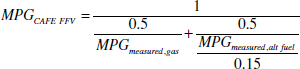
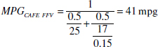
For FFVs, 49 U.S.C. 32905 requires that the fuel economy be calculated similar to dual-fuel vehicles as the harmonic average of the measured fuel economy when running on petroleum fuel and the compliance fuel economy when running on alcohol fuel.11 This is equivalent to assuming that the vehicles would operate 50 percent of the time on petroleum fuel and 50 percent of the time on alcohol fuel, and continues to adjust the alcohol fuel economy by dividing by the fuel content factor, 0.15. For example, for an FFV that is rated at 25 mpg on the petroleum fuel and 17 mpg when operating on an alcohol fuel, the resulting fuel economy for compliance purposes would be 41 mpg:
However, EPA recently finalized an E85 use weighting factor of 0.14 rather than 0.5 for the GHG standard for MY 2016-2018 that manufacturers may use for weighting CO2 emissions, as discussed in Chapter 2. Therefore, the EPA weighting factor for CO2 emissions is more restrictive than the 0.5 weighting factor for CAFE and will limit the application of FFVs.
For dual-fuel natural gas vehicles, 49 U.S.C. 32905, as originally specified by AMFA, requires that the certification fuel economy be calculated as the harmonic average of the tested or measured fuel economy when running on conventional fuel and that when running on natural gas using the same 0.15 volumetric conversion factor as for dedicated alcohol-powered vehicles. The calculation is the same as the FFV. PHEVs are another example of a dual-fuel vehicle. Through 2019, dual-fueled vehicles such as PHEVs are considered to operate 50 percent of the time on gasoline and 50 percent on the alternative fuel. Beginning in 2020, dual-fueled vehicle fuel economy will be weighted by modeled usage of the two types of fuel.
Beginning in MY 2020, EPA has authority under EPCA to develop measurement and fuel economy protocols for the CAFE program (49 U.S.C. 32906) for FFVs and dual-fuel vehicles. Under the MY 2017-2025 Final Rule, EPA finalized its proposal to use the same methodology to weight the alternative and conventional fuel use for both CAFE standards and GHG emissions compliance.12 For ethanol FFVs, manufacturers have the choice of using national average E85 usage data or manufacturer-specific E85 usage data. The default is to use the gasoline fuel economy value for FFVs. For PHEVs and dual-fuel CNG vehicles, the fuel economy weightings will be determined using the Society of Automotive Engineer (SAE) utility factor methodology, SAE J1711. The SAE J1711 utility factor approach is its recommended practice for measuring the exhaust emissions and fuel economy of HEVs.13 The SAE J1711 procedure calculates a utility factor that is based on the vehicles’ electric range and assumes that drivers charge once per day and drive duty cycles similar to the average light-duty passenger vehicle. For example, based on the cycle-specific fleet utility factors, the 2012 Chevrolet Volt PHEV, which has an all-electric range of 38 miles over EPA’s two-cycle certifi-
_____________
10 Dividing Eg by 0.15 yields the PEF = 82,049 Wh/gal.
11 Under EISA, B20 (20% biodiesel and diesel mixture) is also given the same 0.15 fuel content factor as other liquid alternative fuels such as E85 and M85.
12 Note that while the weighting methodology is the same, the CO2 and fuel economy ratings methodologies when operating on an alternative fuel still differ.
13 76 FR 39504-39505 and 40 CFR 600.116-12(b). For more detailed information on the development of this SAE utility factor approach, see http://www.SAE.org, specifically SAE J2841 “Utility Factor Definitions for Plug-In Hybrid Electric Vehicles Using Travel Survey Data,” September 2010.
cation tests, has a combined city/highway cycle utility factor of 0.69, meaning that the average Volt driver is projected to drive about 69 percent of the miles on grid electricity and about 31 percent of the miles on gasoline. The following equations are the J1711 method for petroleum-only fuel economy, the method used for MY 2020 and beyond CAFE fuel economy compliance (Al-Alawi and Bradley 2014):
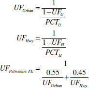
where
UFUrban is the utility factor-weighted fuel economy for the urban drive cycle;
UFU is the urban utility factor, essentially the fraction of urban driving expected to be displaced by an AFV of certain range;
UFHwy is the utility factor-weighted fuel economy for the highway drive cycle;
UFH is the highway utility factor, essentially the fraction of highway driving expected to be displaced by an AFV of certain range;
UFPetroleum FE is the combined city/highway petroleum only fuel economy;
PCTU is the partially charged test fuel economy for the urban drive cycle; and
PCTH is the partially charged test fuel economy for the highway drive cycle.
Using this method, Alawi and Bradley (2014) calculate that a compact car PHEV with 20-mile range (PHEV20) would have a compliance fuel economy of 90 mpg and a compact car PHEV with 60-mile range would have a compliance fuel economy of 226 mpg.
Dual-fueled natural gas vehicles would use the same method as PHEVs to weight the natural gas and petroleum driving portions. EPA provides specific utility factors based on the SAE methodology, which appear identical to the PHEV utility factor (a 50 mi range dedicated natural gas vehicle has a utility factor of 0.689, the same as a PHEV50). A dual-fuel CNG vehicle with a 150-mi two-cycle CNG range would result in a compliance assumption of 92.5 percent operation on CNG and 7.5 percent operation on gasoline. A dual-fuel CNG vehicle with a driving range of less than 30 miles would use a utility factor of 0.50.
CO2 and Fuel Economy Incentives for Advanced Technologies in Full-Size Pickup Trucks
Under the authority of the Clean Air Act and EPCA, EPA provides a per-vehicle CO2 credit in the GHG program and NHTSA provides an equivalent fuel consumption improvement value in the CAFE program for manufacturers that sell significant numbers of large pickup trucks that are mild or strong HEVs or exceed a specific CO2 performance threshold. EPA’s rationale for these incentives is that it believes that the MY 2012-2025 standards will be “challenging for large vehicles, including full-size pickup trucks often used in commercial applications.” EPA’s intent is to pull forward penetration of new technologies, especially hybrids, in the MY 2017-2021 time frame that will help manufacturers meet the more stringent MY 2022-2025 truck standards.
There are four different incentives for advanced technology full-size pickups: two technology-based and two performance-based. The technology-based incentives differ for mild and strong HEV pickup trucks. Mild and strong HEV pickup trucks are defined based on energy flows to the high-voltage battery. The performance-based incentives are for other promising technologies besides hybridization that can provide significant reductions in GHG emissions and fuel consumption, such as lightweight materials. To avoid double-counting, no truck will receive credit under both the HEV and the performance-based approaches.
Mild HEVs are eligible for a per-vehicle CO2 credit of 10 g/mi and an equivalent 0.0011 gal/mi petroleum credit during MYs 2017-2021. To be eligible, at least 20 percent of a company’s full-size pickup production in MY 2017 must be mild HEVs, and that ramps up to at least 80 percent in MY 2021. Strong HEV pickup trucks are eligible for a 20 g/mi credit (0.0023 gal/mi) during MY 2017-2025 if the technology is used on at least 10 percent of a company’s full-size pickups in that model year.
Full-size pickup trucks certified as performing 15 percent better than their applicable CO2 target will receive a 10 g/mi credit (0.0011 gal/mi), and those certified as performing 20 percent better than their target will receive a 20 g/mi credit (0.0023 gal/mi). The 10 g/mi performance-based credit will be available for MY 2017 to 2021 and, once qualifying, a vehicle model will continue to receive the credit through MY 2021, provided its CO2 emissions level does not increase. The 20 g/mi performance-based credit will be provided to a vehicle model for a maximum of 5 years within the 2017 to 2025 MY period provided its CO2 emissions level does not increase. Minimum sales penetration thresholds apply for the performance-based credits, similar to those adopted for HEV credits.
GHG Standard Program Treatment of BEVs, PHEVs and FCEVs
EPA has broader discretionary authority under the Clean Air Act for treatment of AFVs and ATVs, though the basis for the treatment must be grounded in effective reductions in air pollutants. The permanent regulatory treatment for GHG emissions compliance of plug-in hybrid electric vehicles (PHEVs), BEVs, and fuel cell electric vehicles (FCEVs) will use a well-to-wheels analysis (EPA/NHTSA 2012a, 62820). EPA’s GHG standard program has two incentives for BEVs, PHEVs, and FCEVs: zero emission treatment and sales multipliers. For MY 2017-2021, the GHG emission program sets a value of 0 g/mi for the tailpipe CO2 emissions compliance value for BEVs, FCEVs, and PHEVs (based on electricity usage). For MY 2022-2025, the program allows the 0 g/mi treatment for up to a per-company cumulative sales cap tiered as follows: (1) 600,000 BEV/PHEV/FCEVs for companies that sell 300,000 BEV/PHEV/FCEVs in MY 2019-2021; or (2) 200,000 BEV/PHEV/FCEVs for all other manufacturers. Starting with MY 2022, the compliance GHG emissions value for BEVs, FCEVs, and the electric portion of PHEVs in excess of individual automaker cumulative production caps must be based on net upstream accounting of CO2 emissions.
The GHG standard program also provides a sales multiplier that allows a manufacturer to count each BEV/PHEV/FCEV/compressed natural gas (CNG) vehicle as more than one vehicle in the manufacturer’s compliance calculation. EPA’s rationale for providing multipliers is “to provide temporary regulatory incentives to promote advanced vehicle technologies” (EPA/NHTSA 2012a, 62650). EPA provides CNG vehicle multipliers since it believes that the infrastructure and technologies for CNG vehicles could serve as a bridge to use of advanced technologies such as hydrogen fuel cells. BEVs and FCEVs start with a multiplier value of 2.0 in MY 2017 and phase down to a value of 1.5 in MY 2021. PHEVs and CNG vehicles start at a multiplier value of 1.6 in MY 2017 and phase down to a value of 1.3 in MY 2021.
The impact of these zero emission treatment and multipliers is to effectively provide a CO2 credit toward a manufacturer’s fleet average compliance calculation. For every 1 percent of total passenger car production, the zero emission treatment alone is worth 2.1 g/mi starting in MY 2017, declining to 1.4 g/mi in MY 2021. When the 2.0 multiplier in MY 2017 is considered, the credit is worth 4.2 g/mi.
Appropriateness of Credits for Alternative Technologies
Battery Electric Vehicle Incentives
The CAFE incentives for BEVs provide a fuel economy credit toward a manufacturer’s compliance, thereby reducing the average fuel economy required of its conventional vehicle fleet. Based on the fuel economy standards for passenger cars in the MY 2017-2025 Final Rule, the committee estimates that if a manufacturer chose to produce 1 percent BEVs, it could reduce the fuel economy of its conventional fleet by 0.35 mpg in MY 2017 and 0.47 mpg in MY 2025. The incentives effectively create a trade-off: Current petroleum consumption will be higher under the rule with the PEV incentives, in exchange for the potential for greater petroleum reductions in the future due to the deployment of PEVs. The value of the credits may be thousands of dollars per vehicle. This incentive may drive additional deployment of PEVs. But this may not be the most cost-effective way to increase the number of alternative fuel vehicles in the long run.
California’s Zero Emission Vehicle (ZEV) requirements will also influence the rate of adoption of PHEVs, BEVs, and FCEVs by auto manufacturers. Large-volume manufacturers will be required to supply 15.4 percent of the vehicles they sell in California and other participating states as zero emission vehicles (i.e., as either PEV or FCEV by 2025 (CARB 2012)). As of 2014, nine states in addition to California are adopting the ZEV standards, representing a total of about 28 percent of the new vehicle market in the United States (ZEV Program Implementation Task Force 2014). The volumes of PHEVs, BEVs, and FCEVs estimated by the California Air Resources Board to be produced in compliance with the ZEV mandate in California are illustrated in Figure 10.5. The ZEV mandate does not directly impact the CAFE standards but will influence the way these manufacturers meet the federal CAFE/GHG standards. The vehicles that manufacturers sell to comply with the ZEV mandate will form a part of their compliance with the CAFE/GHG standards, meaning that they will need fewer fuel economy improvements from their conventional vehicles than would have been required without the ZEV mandate.
MY 2020 and Beyond Methodology for FFVs and Dual-Fuel Vehicles
The impact of the utility factor approach for PHEVs and dual-fueled CNG and the demonstration of actual usage for FFVs will be to increase the credits for PHEVs and dual-fuel CNG vehicles and decrease the credits for FFVs. The Agencies believe that while weighting to better reflect real-world usage is a major change, this change “orients the calculation procedure more to the real-world impact on petroleum usage, consistent with the statute’s overarching purpose of petroleum conservation” (EPA/NHTSA 2012a, 62829).
Many analysts have pointed out that the current crediting system for FFVs that assumes a 50/50 split of alcohol to petroleum has led to the unintended consequence of increasing petroleum dependency since only a small fraction of FFVs actually uses E85 (DOT et al. 2002; GAO 2007; Liu and Hefland 2009). Tying FFV credits to actual use of an alternative fuel is consistent with DOT et al. (2002) and GAO (2007) recommendations. DOT et al. (2007) recommended “linking the CAFE credit to actual alternative fuel used.” GAO (2007) recommended that the dual-fuel program should
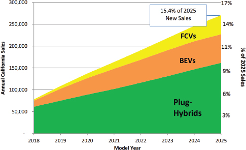
FIGURE 10.5 Annual California sales for MY 2018-2025 expected for ZEV regulation compliance, showing projected PHEV, BEV, and FCEV sales.
SOURCE: CARB (2011).
be “eliminated or revised.” It recommended “lowering the credit to more accurately reflect how often these vehicles are actually run on alternative fuels could be appropriate.”
Adoption of the “utility factor” method to credit PHEVs and dual-fuel CNG vehicles is an improvement over the previous method of assuming a 50/50 split. However, while the utility factors are based on actual survey data of travel behavior, this will not necessarily correlate with alternative fuel refueling behavior in the real world. The Agencies postulate that if a driver spends the extra money on PHEV or CNGV, he/she is more likely to use the alternative fuel. This assumption may hold well for PHEVs that have multiple refueling options (home charging). In fact, early adopters of the Chevrolet Volt, as studied in the EV Project, drive on average 75 percent on electricity, more than the utility factor predicts (ECOtality 2013). The assumption that utility factors accurately predict alternative fuel usage behavior may not be as reasonable for a dual-fuel CNGV if infrastructure is not readily available.
APPROACH AND METHODOLOGY USED TO SET STANDARDS AND EVALUATE COSTS AND BENEFITS
Introduction
The Agencies use a series of models to carry out the quantitative analysis necessary to estimate feasible levels of fuel economy increases and GHG reductions and their costs. Each Agency models plausible technology changes to forecasted future fleets that would result in compliance for each manufacturer. The structure of the analytical methodology is similar for both of the Agencies and is illustrated in Figure 10.6. Data on the performance of vehicle components and systems, including engine maps, aerodynamic drag coefficients, and other information, are inputs to the full vehicle simulation model. The full vehicle simulation model predicts the impacts of advanced fuel economy and GHG technologies on fuel consumption and emissions for seven base vehicles representing seven vehicle classes. These data are used to calibrate a simpler lumped parameter model that can be used to estimate impacts for millions of technology-vehicle combinations. These impacts, together with estimated technology costs, are used by the Agencies’ compliance models (Volpe and OMEGA) to estimate manufacturer-specific compliance with fuel economy and emissions standards.
In the compliance models, technologies are ordered by cost effectiveness subject to engineering and manufacturing constraints. The models iterate, adding technologies to individual makes, models, and engine-drivetrain configurations with the objective of achieving cost-effective reductions in petroleum use and GHG emissions. Through the use of these models, the Agencies developed what the committee termed the EPA/NHTSA compliance demonstration path representing a cost-effective set of technologies that automobile manufacturers could adopt to meet the standards. These compliance demonstration paths are broken down by individual manufacturer and by model year. These are reported as the technology penetrations by manufacturer and year in the Final Rule and in supporting documents. Although the Agencies’ analysis demonstrates a possible technology path to compliance, each OEM will plot its own future course to compliance. Thus, what the
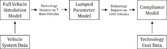
FIGURE 10.6 Simplified diagram illustrating the Agencies’ methodology for setting standards.
Agencies’ analysis shows is a demonstration of possibility, not a forecast of the future.
Baseline and Reference Vehicle Fleets
In addition to establishing the technologies that could be implemented for fuel economy by 2025, the Agencies also evaluated the costs and benefits of the rule. Developing both the technology paths and the costs and benefits used the concepts of the null, baseline, and reference vehicle fleets. The committee developed Figure 10.7 to aid in its understanding of the relationship among the null vehicle, baseline fleet, reference fleet, reference case, and control case.
The Agencies developed the null vehicle package as a reference point against which effectiveness and cost can be consistently measured across compliance models (Olechiw 2014). Chapter 8 defines the null vehicle concept and describes how the baseline fleet is built up from a null vehicle to an estimate of the actual fleet as it existed in either 2008 or 2010. This building up of the null vehicle to the actual fleet is shown Step 2 of Figure 10.7 using grey squares to represent the technologies added to the individual vehicle models. One complexity in building the baseline fleet for the 2017-2025 CAFE/GHG standards is the use of two baseline years. This was done in large part due to the effects of the economic recession on the 2008 sales and sales mix. The recession not only caused a drastic reduction in vehicle sales but altered the distribution of sales and led to the termination of certain vehicle makes. Thus, the Agencies developed a second baseline fleet using 2010 certification data.
Once the baseline fleet for 2008 or 2010 had been defined, technologies were added to the individual vehicle models within an OEM’s lineup until, combined with projected sales volumes for each model, each manufacturer’s car and truck sales met the 2016 CAFE/GHG standards. The OMEGA and Volpe models are used for this purpose. The projected fleet that reached compliance in 2016 defined the reference fleet for 2017. Figure 10.7 represents the technologies added to move from the baseline to reference fleets in Step 3. The varying numbers of technologies and lengths of time between technology additions in Figure 10.7 illustrate that each model may start at a different level of technology and may apply a different number of technologies at different times.
The 2017 reference fleet formed the basis of both the reference case and the control case. To make the reference case, the reference fleet was futured by assuming no technology improvements and no improvements in fuel economy beyond 2016, but allowing for forecasted changes in vehicle sales and class/model mix over time. The 2017 reference fleet was also used to form the control case, in which technologies were added to increase fuel economy and reduce GHG emissions from 2017 to 2025 to meet the 2025 standards. The difference between the control case and the reference case amounted to the Agencies’ assessment of the costs and benefits of the standards.
The Agencies’ use of the two 2008 and 2010 baseline fleets is a step toward acknowledging the uncertainty of future vehicle markets. The large differences between the 2008 and 2010 data (only 2 years apart) is a reminder of the difficulty of forecasting the vehicle market as far as 15 years into the future. Makes and models will come and go, the popularity of vehicle classes will change, new vehicle types will be created, and existing ones will fade away. The committee knows of no methods for accurately predicting the volume, composition, and technology of light-duty vehicle sales 15 years into the future; however, important economic uncertainties should be included as a sensitivity analysis in the reference case. Also, there is potential for economic–engineering models to use forecast data on cost, effectiveness, and demand elasticities to make useful uncertainty analyses of the broad effects of the rule. The price of gasoline, for example, is critically important to the costs and benefits of the rule, and various assumptions about the price of gasoline should be included among the economic uncertainties evaluated. Analyzing the nature and degree of uncertainty over similar time periods in the past may provide useful guidance about the nature and degree of uncertainty that can be expected in the future.
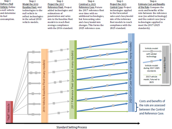
FIGURE 10.7 Schematic illustrating the Agencies’ definition of null vehicles, 2010 baseline fleet, 2017 reference fleet, reference case, and control case used to evaluate the CAFE/GHG standards. Each arrow represents a vehicle model progressing through time. The slanting arrows represent increasing fuel economy over time. Technologies added to the models are represented by squares. In setting the standards, the agencies define a null vehicle, a 2008 or 2010 baseline fleet modeled on the real 2008 and 2010 fleets, and a 2017 reference fleet projected to comply with the 2012-2016 standards. The Agencies then form a reference case, representing the 2017 reference fleet progressing through time with no added technologies, and a control case, representing the 2017 reference fleet progressing through time with added technologies to meet the more stringent standards. The costs and benefits of the rule are determined between the reference and control cases, summed over the sales-weighted vehicle models.
Reference Case and Implications for Estimating Costs and Benefits
The costs and benefits of improved fuel economy as a result of the rule from 2017 to 2025 are estimated relative to a reference case that assumes some growth over this period in the overall vehicle fleet and a relative shift toward cars and away from trucks. It assumes, however, that there will be no changes after 2016 to the fuel economy of individual model vehicles. The implication of comparing the improvements in each year to the reference case is that in the absence of the rule, the fuel economy of the fleet would not have changed at all through the 2017 to 2025 time period—fuel economy would have remained through time at its 2016 level. The Agencies acknowledge this assumption and believe it is consistent with consumer choices from 1984 to 2004 (see Figure 9.1).
Using the 2016 vehicle as a reference also implicitly assumes that there would be no other improvement to other vehicle characteristics in the absence of the standards. This is equivalent to a reference case with no further technical change in the vehicle market from 2017 to 2025. An alternate reference case for the benefit cost analysis would account for
a rate of technological progress similar to what has occurred in the past. The rate of technological progress in vehicle attributes and efficiency has been strong and continual over the past 30 years, as shown in Figure 9.1. Also, EPA (2014c) provides further evidence of past trends.
Developing a reference case that reflects technological progress over time is important for attempting to account for costs and benefits that might be left out of the analysis. The reference case with no fuel economy changes should instead include some attempt to measure improvements in other vehicle attributes likely to occur over time. Then, with the introduction of the rule, and all improvements going toward fuel economy, there will be opportunity costs in terms of the other attributes that are forgone. NHTSA acknowledges this issue in the Final Rule when they state, “the true economic costs of achieving higher fuel economy should include the opportunity costs to vehicle owners of any accompanying reductions in vehicles’ performance, carrying capacity, and utility, and omitting these will cause the agency’s estimated technology costs to underestimate the true economic costs of improving fuel economy” (EPA/NHTSA 2012a, 62988). The committee recognizes the difficulty of determining an appropriate reference fleet over time and of estimating the opportunity costs. But there are various approaches that could be developed to incorporate such forecasts in the reference fleet. There is past evidence about the rate of technological change that provides some guidance. There are continuing efforts to improve estimates to the value of fuel economy and other vehicle attributes to consumers that could inform the estimates of opportunity costs.
Technology Impact Estimation
Estimating the impacts of technologies with the potential to reduce fuel consumption and greenhouse gas emissions is complicated by three issues:
- Implementations of technological concepts differ across manufacturers and even across vehicles made by the same manufacturer.
- Technologies often have secondary effects on vehicle attributes that may require additional engineering or design changes that affect fuel economy.
- Dynamometer testing of two vehicles with and without the technology in question but that are otherwise identical is generally not possible.
As a consequence, estimating the impacts of technologies on fuel consumption always involves a degree of uncertainty.
Full Vehicle Simulation Modeling
The National Research Council’s (NRC’s) 2011 report on fuel economy technologies recommended that the Agencies make use of full system simulation modeling (a.k.a. full vehicle simulation) to estimate the impacts of fuel economy technologies:
Full system simulation (FSS), based on empirically derived powertrain and vehicle performance and fuel consumption data maps, offers what the committee believes is the best available method to fully account for system energy losses and synergies and to analyze potential reductions in fuel consumption as technologies are introduced into the market. (NRC 2011, 155)
The Agencies have endeavored to follow this recommendation and made extensive use of full vehicle simulation modeling in their technical analyses in support of the 2017-2025 rule. Simulation analyses for the 2011-2016 rule were carried out by Ricardo, Inc. using its commercially available simulation model, EASY5. While the EASY5 model is commercially available, Ricardo used proprietary input for the engine maps, transmission efficiencies, and shift schedules for the EPA analysis. Those analyses included 26 technology packages applied to five vehicle classes. For the 2017-2025 rule, an additional 107 vehicle packages were simulated by the same consulting firm for seven vehicle classes (Ricardo 2011). In addition, a design of experiments method was used to vary input parameters to develop data for predicting the combinations of factors such as engine size and final drive ratio that would yield the greatest reduction in fuel consumption while meeting the requirement of performance equivalent to the baseline and reference fleets (EPA 2012a, 3-55). The simulations included four advanced engine concepts, five advanced transmissions, and two hybrid vehicle architectures (EPA 2012a, Tables 3-5 and 3-6).
The Agencies have made substantial progress toward the goal of full system simulation modeling for every important technology pathway and for every vehicle class. Full vehicle simulation modeling has limitations, however. First, because it is skilled-labor- and data- intensive, it is also relatively expensive. Second, the expertise and software resources have historically been found only in the OEMs and industry research and consulting firms. Some of the necessary information held by these firms is proprietary, which constrains the ability of the Agencies to obtain peer review and to accomplish full disclosure. Third, full vehicle simulation modeling, as envisioned by the 2011 NRC committee, can only be carried out for technologies that have already been competently incorporated into at least one vehicle. Only then can the performance and data maps be empirically derived. For technologies that have not been implemented, existing engine maps and other key inputs can be modified by expert judgment, which makes validation difficult. A preferred alternative to this approach is to use a detailed engine model calibrated to an existing engine map, to develop maps for engines that have not been developed in hardware (as was done in the committee’s University of Michigan full system
simulation discussed in Chapter 8). The Agencies should consider adopting this approach for technologies that have not been implemented. Finally, due to resource limitations, full vehicle simulation modeling is not feasible for every one of the approximately 1,000 vehicles in the baseline or reference fleets. Because the technologies present on other vehicles will differ from the configuration used in the simulation modeling (and their implementations will vary as well), other methods must be used to estimate the impacts on each and every vehicle in the baseline and reference fleets.
Validation of the full vehicle simulation model runs is difficult because advanced technologies are sometimes not available in an actual vehicle, especially in the full range of combinations considered in the modeling. The EPA conducted an external peer review of the modeling by Ricardo, Inc., in which the review panel expressed frustration with their lack of access to proprietary data and models. The EPA reported to the committee on actions it has taken to validate its simulation modeling results by comparisons with dynamometer tests on existing vehicles (EPA 2014b). The EPA also reported that it is developing its own simulation model named ALPHA, in order to allow full public disclosure of the model and its input data (EPA 2012a).
Lumped Parameter Modeling
Lumped parameter models simplify the representation of a complex system by using a smaller number of elements and associated parameters to approximate the behavior of the full system. The objective of lumped parameter modeling of vehicle fuel economy is to represent the synergies in reductions of energy losses among technologies in a model that is orders of magnitude less complex than a full vehicle simulation model. The EPA developed a lumped parameter model in order to estimate the impacts of combinations of technologies on the baseline and reference fleets. In 2012, NHTSA and EPA used outputs of the lumped parameter model to calibrate inputs to NHTSA’s Volpe model and EPA’s OMEGA model.
EPA’s lumped parameter model represents the conversion of chemical energy in fuel to thermal and mechanical energy in the vehicle. It quantifies the losses of energy in the vehicle system: the determinants of the forces the vehicle must overcome to accomplish the dynamometer test cycles as well as energy dissipated in braking (EPA 2012a, 3-69). The baseline vehicle is described by a fixed percentage of chemical energy going to each category of energy use (loss), including thermodynamic losses, exhaust heat, pumping losses, engine friction losses, transmission losses, vehicle road load losses, and inertial losses. Fuel economy technologies reduce specific categories of energy losses by a certain percentage. This avoids double counting of benefits and helps ensure that the overall impact estimates do not violate physical laws. Because it is far less complex than full vehicle simulation models, the lumped parameter model could be used to estimate impacts on all 1,000 or so vehicles and millions of vehicle–technology combinations for the baseline and reference fleets. These results are used by the OMEGA and Volpe models in estimating compliance with the fuel economy and emissions standards.
The EPA’s lumped parameter model is calibrated to the full vehicle simulation results. This is presumably done by adjusting the energy loss shares; however, the technical support document does not describe the calibration process in sufficient detail to evaluate it. EPA presented to the committee a sample of comparisons between the lumped parameter model predictions and the 2011 Ricardo simulation results (EPA 2014b). The comparisons supported EPA’s assertion that the lumped parameter model predictions are within 3 percent of the full simulation modelling results for the seven baseline vehicles and “with a few exceptions” within 5 percent for advanced technology packages.
Cost Estimation
From the perspective of the costs and benefits of fuel economy and GHG standards, accurately estimating costs is as important as estimating technology impacts. The methods the Agencies use for estimating direct and indirect costs over time are discussed in Chapter 7. This section addresses the way costs are used in the methodology for setting standards. Technology costs are used to calculate one or more cost-effectiveness indices for each technology. Conceptually, cost-effectiveness is defined as the incremental cost per percent reduction in fuel consumption ($/% FC). A high cost-effectiveness can be expressed either as a high fuel consumption reduction effectiveness/cost or as the inverse, a low cost/fuel consumption effectiveness, as is reported in the EPA RIA and in the example pathways in Chapter 8. Technologies are applied to vehicles in the compliance models in order of cost-effectiveness, subject to a number of constraints. The constraints include the applicability of a technology to a specific vehicle class, its availability in the year being simulated, its compatibility with other technologies in use on the vehicles, and whether it requires that other technologies be implemented prior to its use. A technology’s retail price equivalent cost includes both direct manufacturing and indirect costs.
Compliance Models
The Agencies are obligated to provide a least-cost compliance path that shows how each OEM might comply with the standards, not necessarily the path they will actually follow. Each Agency has its own model for estimating compliance with fuel economy and GHG standards and the costs and benefits thereof. Both models are available to the public. The NHTSA model (a.k.a. the Volpe model) was developed for earlier rulemakings and revised in 2012 (NHTSA 2012a). The EPA’s OMEGA model is similar with respect to in-
puts and outputs and the logic for determining compliance (OMEGA). Both models apply technologies to the baseline and reference fleets in order of cost-effectiveness, subject to constraints to represent availability, applicability, and engineering logic. Both models calculate manufacturer-specific standards based on the footprints and sales of the vehicles in the baseline and reference fleets using the footprint versus fuel economy and GHG functions. Neither model estimates the impacts of fuel economy or GHG standards on the mix of vehicles sold, although both Agencies have research projects under way to investigate the feasibility and value of estimating such impacts. The models iteratively apply technologies to each manufacturer’s vehicles until the specified standard is met or the available technologies are exhausted. The models differ in their methodology for adding technologies to a vehicle. The Volpe model applies technologies to every vehicle model within each manufacturer’s fleet using decision trees until the manufacturer’s fleet achieves compliance. In contrast, the OMEGA model develops “master sets of technology packages” for each vehicle class. The OMEGA model applies these packages to the vehicle classes in the entire U.S. fleet rather than by manufacturer, as in the Volpe model. The Volpe model also allows manufacturers to pay a penalty if the cost of meeting the standard exceeds the statutory fine for noncompliance. Since that feature is not an option under the GHG regulations, the Volpe model allows it to be disabled.
Both models take account of the availability of technologies in time and the normal redesign cycles for vehicles. Technologies may be designated as applicable or not applicable to each class of vehicle. Each technology is also described by an earliest year in which it becomes available for use and a later year in which it will no longer be available. For recently introduced technologies, limits can be placed on how rapidly the technology can be adopted. One difference between the OMEGA and Volpe models is that the Volpe model’s algorithm calculates compliance by model year whereas the OMEGA model applies technologies for a “redesign cycle,” which is assumed to be approximately 5 years.
According to EPA, “OMEGA assumes that a manufacturer has the capability to redesign any or all of its vehicles within this redesign cycle. OMEGA does not attempt to determine exactly which vehicles will be redesigned by each manufacturer in any given model year” (2012b, 6). This method does not permit evaluation of banking, borrowing, and credit trading, features that have been shown to be important to manufacturers’ abilities to cost-effectively achieve compliance with fuel economy and emissions standards (Rubin et al. 2009; Bunch and Greene 2011; Liu et al. 2014). It also does not permit a year-by-year analysis of the industry’s investment requirements.
Once a final level of fuel economy is achieved, the models estimate the social costs and benefits of the standards. These include both private costs and benefits to individual consumers and external costs and benefits that accrue to society as a whole. The external benefits of the rule include the value of reductions in GHG emissions, the energy security benefits of reduced petroleum consumption, and health improvements due to particulate matter reductions.14 There are also some small external costs in terms of more congestion and accidents from more driving due to the rebound effect.15 The private costs to consumers are the higher upfront cost of vehicles (termed program costs), and the private benefits are the fuel savings, the savings from less frequent refueling, and the value of additional miles driven due to the rebound effect. The private benefit of the fuel savings is by far the largest benefit, though it may not be considered by car buyers at the time of purchase, as discussed at length in Chapter 9. The relative sizes of the private and public (external) costs and benefits associated with the lifetimes of 2017-2025 MY light-duty vehicles, assuming a 3 percent discount rate, are shown in Figure 10.8.
The costs of petroleum dependence and greenhouse gas emissions are particularly important because they represent the primary motivation for the standards. The rulemaking lists the benefits of reduced oil consumption as “reduction in petroleum market externalities” (EPA/NHTSA 2012a, 63080), indicating a misunderstanding of the nature of oil dependence costs. It is important to recognize that the salient market failure in the case of oil dependence is imperfect competition. Imperfect competition is not an externality and should not be estimated as if it were. The economic harm done by higher than competitive market prices has two components: (1) reduced GDP due to the increased economic scarcity of petroleum and (2) a transfer of wealth from oil-importing economies to oil-exporting economies (Greene 2010). The second component is not an economic loss from a global perspective but is an economic loss from the perspective of the U.S. economy. This fact has apparently created some confusion about how to add up costs and benefits.16 Petroleum dependence can also impose external costs associated with military expenses.
The Agencies estimate a variety of different costs to petroleum dependence, including macroeconomic costs imposed by disruptions in oil imports, higher cost of oil due to U.S. demand in the world market (termed the monopsony component, discussed below), and military costs to secure oil imports from unstable regions and maintain the Strategic Petroleum Reserve. The Final Rule notes that only the macroeconomic disruption costs are incorporated into the cost benefit analysis (EPA/NHTSA 2012a, 62717). The Agencies
_____________
14 EPA estimated PM2.5 reductions because the net emissions reductions from reduced fuel refining, distribution, and transport is larger than the emissions due to increased VMT and increased electricity production (EPA/NHTSA 2102a, 62899).
15 The rebound effect is an increase in vehicle use as a consequence of the reduction in the cost of energy per mile of driving due to increased fuel economy.
16 The OMEGA model discussion also appears to confuse the costs of oil import dependence with the costs of oil dependence. The economic costs of oil dependence are a function not only of the quantity of imports but also of the total quantity of oil consumed throughout the economy.
17 The Agencies did include an estimated military cost in their sensitivity analysis but this does not adequately address the need to consider national defense and foreign policy costs.
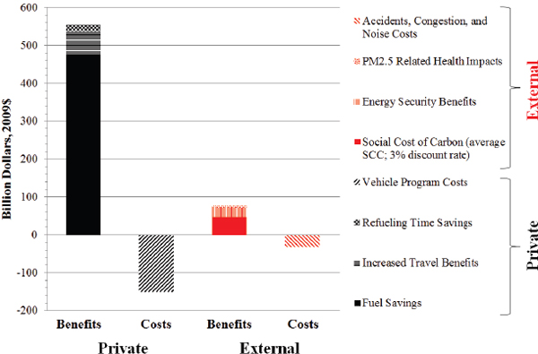
FIGURE 10.8 Distribution of lifetime private benefits and costs (black) and external benefits and costs (red) of 2017-2025 MY light-duty vehicles under the standards, using a 3 percent discount rate.
SOURCE: Data from EPA/NHTSA (2012a, Tables III-104 and III-105).
justify excluding the military security costs because they are difficult to quantify. The difficulty of estimating national defense and foreign policy costs due to oil dependence has been noted elsewhere (NRC 2010). Difficulty of estimation may lead to estimates that are uncertain but it does not imply zero cost as assumed in the Final Rule (EPA/NHTSA 2012a, 63088).17
In considering the standards’ GHG and oil dependence benefits, the Agencies excluded what are termed “monopsony benefits” (EPA/NHTSA 2012a, 62939). Monopsony benefits measure the benefit to the U.S. economy of a reduction in the world price of oil due to reductions in U.S. oil demand brought about by the standards. Because the U.S. accounts for more than one-fifth of the world’s petroleum consumption, large changes in U.S. demand can affect world prices in both the short and long run. The Agencies quantified the monopsony benefit at $9.77/bbl, slightly larger than the $8.26/bbl benefit attributed to reduced disruption of oil supplies (EPA/NHTSA 2012a, 62939). In accounting for costs and benefits of the rule, the oil disruption benefit was incorporated as an external energy security benefit and the monopsony benefit was not incorporated. The justification for excluding the monopsony benefit was that it is a transfer and not a benefit from the perspective of the global economy. The reasoning was that if one includes the full global benefit of reduced U.S. GHG emissions, one must also take the global perspective when it comes to the transfer of wealth due to higher than competitive oil market prices. Since the U.S. economy’s gain is canceled by a corresponding loss of revenue to oil exporters, there is no monopsony benefit from the global perspective. The fallacy in this reasoning resides in insisting that the scope of the two problems, oil dependence and climate change, must be the same. In fact, oil dependence is a national concern of the United States. Like national defense, it is inherently adversarial (i.e., oil consumers against producers using monopoly power to raise prices). The problem of climate change is inherently global and requires a global solution. If each nation considered only the benefits to itself in determining what actions to take to mitigate climate change, an adequate solution could not be achieved. Likewise, if the U.S. considers the economic harm its reduced petroleum use will do to monopolistic oil producers it will not adequately address its oil dependence problem. Thus, if the United States is to solve both of these problems it must take full account of
the costs and benefits of each, using the appropriate scope for each problem.
Uncertainty
Estimating the potential for future fuel economy improvement and its costs and benefits is complex and uncertain. As this report has repeatedly noted, estimating even the current costs and impacts of fuel economy technologies involves substantial uncertainty. The Agencies discuss these sources of uncertainty at length in Section IV of the Final Rule, as well as within the Agencies’ respective RIAs (EPA/NHTSA 2012a; EPA 2012c; NHTSA 2012b). The Agencies have done sensitivity and uncertainty analysis for the 2017-2025 CAFE/GHG standards in theses RIAs. EPA conducted a sensitivity analysis regarding benefits from reducing GHG emissions and fuel savings for different assumptions of the rebound rates—that is, the increase in vehicle use that results if an increase in fuel efficiency lowers the cost per mile of driving (EPA 2012c). It also looked at the sensitivity of the regulation’s benefits under varying assumptions concerning health impacts of air pollution and the global warming potential of various GHGs. NHTSA performed a sensitivity analysis on fuel prices and a probabilistic uncertainty analysis using Monte Carlo simulation. The Monte Carlo analysis included uncertainties in (1) technology costs, (2) technology effectiveness, (3) fuel prices, (4) manufacturers’ decisions to produce vehicles with higher fuel economies than mandated by the CAFE standards, (5) VMT, (6) passenger car share of the new market, (7) value of oil consumption externalities, and (8) rebound effects (NHTSA 2012b). The results of the NHTSA probabilistic assessment shows that, for a range of assumed discount rates, there is a high degree of certainty (99 percent) that higher CAFE standards will produce a net societal benefit in each of the combined fleet model years covered by this rule.
A more comprehensive modeling of uncertainty would integrate all the components noted above, including uncertainty about the baseline and reference vehicle fleet size and composition. Looking ahead to 2025 and 2030 brings in additional sources of uncertainty:
- The pace and direction of future technological progress,
- Current and future consumer behavior and preferences,
- Future market conditions, including the prices of key commodities from oil to aluminum,
- Future regulatory initiatives, and
- The impacts of global climate change and the importance of GHG mitigation.
At present, it is not clear how to carry out such a comprehensive uncertainty analysis. The committee is well aware of the challenges posed by assigning probability distributions to point estimates of costs and fuel consumption impacts. Introducing a much wider array of uncertain parameters would not only magnify the challenge but create a far greater complication: representing the relationships among the factors.
The committee could not conduct a probabilistic uncertainty analysis given resource and time constraints. The committee throughout its report emphasizes where it sees important uncertainties for both the technology benefits and costs as well as for other factors that will impact the cost and implementation of the new standards. In particular, Chapter 9 emphasizes uncertainties in the estimation of how consumers value fuel economy and other vehicle improvements and how willing consumers are to purchase innovative technologies. Though the committee could not quantify these uncertainties, they are noted throughout the report as topics for follow-up analysis by the Agencies.
Agency Coordination
The Final Rule supporting documents reflect a high degree of coordination between the Agencies with respect to data, methods, and premises. Differing regulatory mandates require effort in coordination of analysis, and the Agencies retain different compliance models to allow them to represent the different requirements of the CAFE and Clean Air Act laws. Multiple support documents are required of NHTSA and EPA in the process of setting the standards due to differing regulatory mandates. The analysis and documentation in support of the rule contains redundancies and inconsistencies. Redundancies, such as development of different full vehicle simulation models, are a waste of limited resources and should be consolidated. Redundancies can also lead to inconsistencies, which should be minimized to ease understanding of and compliance with the standards.
Reconciling GHG and CAFE Treatment of Alternative Fuel Vehicles
Fuel economy and GHG emissions are regulated by two Agencies, NHTSA and EPA. The motivations for these regulations include energy efficiency, reduction of GHG emissions, and energy security. The standards have been harmonized such that for gasoline-powered vehicles excluding AC credits, the CAFE and GHG objectives are consistent based on the relationship between a given volume of gasoline and the associated mass of CO2 produced upon combustion. Difficulties arise when other fuels are used for propulsion as the standards are not harmonized with those fuels in mind. For example, alternative fuels benefit energy security but not necessarily GHGs. The first challenge in regulating under two objectives lies in misalignment between the petroleum reduction and GHG benefits for some AFVs. For example, domestically-produced fuels such as ethanol and natural gas provide substantial energy security benefits but only modest GHG benefits. A second complication for regulating under two metrics is that to appropriately account for the GHG emissions of vehicles using a variety of fuels, upstream
emissions not produced at the tailpipe must be included. The GHG benefits for BEVs and FCEVs, for example, are entirely dependent on how the electricity or hydrogen is produced. The GHG benefits of natural gas and ethanol will also be significantly impacted by their upstream emissions.
The first complication in regulating under two metrics is harmonizing standards from a petroleum consumption and GHG emissions perspective for vehicles powered by fuels other than gasoline, such as ethanol, electricity, hydrogen, or natural gas. For example, BEVs must be assigned a compliance mpg-equivalent value even though they use no petroleum onboard. Compliance fuel economy of electric vehicles and other AFVs are increased using a 0.15 divisor (equivalent to multiplying fuel economy values by 6.67), which appears to be based on providing the same incentive multiplier as E85 and is not directly related to the petroleum consumption of electricity, hydrogen, or natural gas. This is equivalent to assuming that all alternative fuels provide an 85 percent reduction in GHGs per unit of energy. For FFVs, where the 0.15 divisor is related to the petroleum content of the alternative fuel, the regulatory treatment assumed 50 percent use of E85 and 50 percent use of gasoline, when in fact very few consumers use E85. As noted previously, this treatment is appropriately being phased out. While alternative fuels can lead to major discrepancies between the CAFE and GHG benefits, diesel vehicles also present a complication. Diesel combustion results in more carbon dioxide emitted per gallon than gasoline, so a diesel vehicle that meets the CAFE target for its size would exceed its GHG target. Even gasoline vehicles rely on corrections to the GHG/CAFE relationship—for example, through air conditioning emissions credits.
The second complication with regulating alternative fuel vehicles is how to appropriately account for upstream emissions of GHGs and consumption of petroleum. A well-to-wheels analysis is appropriate to assess and compare the very different upstream GHG and petroleum impacts of fuels. Light-duty vehicles of all fuel types are assessed for fuel consumption and tailpipe GHG emissions in the compliance test cycles described earlier in this chapter. For CAFE and GHG compliance of gasoline and diesel vehicles, no direct accounting is made for upstream emissions and petroleum consumption from refining or transportation of petroleum. As described earlier in the chapter, the permanent GHG regulatory treatment of PHEVs, BEVs, and FCEVs will use a well-to-wheels analysis and corrects for the upstream GHG emissions of a comparable gasoline vehicle in order to provide equitable treatment. Up to a certain cumulative production volume by a manufacturer, however, these well-to-wheels emissions are not taken into account as a temporary regulatory incentive, as discussed previously in the chapter. The CAFE program also accounts for upstream energy consumption, but not petroleum consumption, for PHEVs, BEVs, and FCEVs. For consumer information, a well-to-wheels analysis of GHG emissions for all vehicle types, including gasoline, diesel, and alternative fuels, is currently provided at Fueleconomy.gov.
It is not clear how to permanently resolve the differences in energy security and GHG benefits of all alternative fuels. Also, although permanent regulatory treatment of PHEVs, BEVs, and FCEVs is on a well-to-wheels basis, this is not implemented at current production volumes, nor is it used for vehicles powered by other fuels such as natural gas and ethanol. Well-to-wheels analysis provides a way to compare the GHG and petroleum impacts of a variety of fuels. While the Agencies have made commendable efforts to harmonize the CAFE/GHG national program, the committee finds that having two metrics, both greenhouse gases emissions and petroleum consumption, creates conflicts that can complicate regulations and compliance. The committee notes the strong complementarity between the two objectives. It appears that reducing the total GHG emissions (well-to-wheels) from light-duty vehicles to levels that would appropriately address the problem of climate change would also adequately solve the oil dependence problem. The Agencies should study the potential benefits, costs, and risks of establishing a standard based on a single metric that achieves both GHG and petroleum reductions in addition to continued efforts to harmonize the two regulations.
Finding 10.1 In the current assessment of the effects of the new rules, the footprint standard is assumed to have no effect on vehicle size, or on the mix of vehicle size and market shares. However, the rules could well have effects on costs and revenues for vehicles of different types and sizes, which may lead to changes in vehicle design and sales. Preliminary studies of this issue show a range of results, from little effect on the vehicle sales mix to changes in design and sales mix, leading to a larger footprint. The effects of the rule on vehicle sales mix and redesign is important because larger vehicle sizes could reduce the benefits of the rule in terms of reductions in oil consumption and GHG emissions.
Recommendation 10.1 The Agencies should monitor the effects of the CAFE/GHG standards by collecting data on fuel efficiency, vehicle footprint, fleet size mix, and price of new vehicles to understand the impact of the rules on consumers’ choices and manufacturers’ products offered. The Agencies have already initiated this effort, and it should be continued as a first step toward understanding the overall effect of the rule on vehicle size and size mix. Without analysis of manufacturers’ and consumers’ choices, however, it will be difficult to isolate the effects of the rule alone. Economic-engineering models of manufacturer decision making that take into account costs and consumer responses should also be developed as part of the assessment of the rule.
Finding 10.2 The empirical evidence from historical data appears to support the argument that the new footprint-based standards are likely to have little effect on vehicle safety and
overall highway safety. If the size mix of vehicles remains roughly the same, then a reduction in the weight of vehicles is not generally associated with greater societal safety risks. To the extent the size mix and design of vehicles changes substantially, the effects on safety are not known. There will need to be continuing empirical analysis of the safety outcomes as vehicle designs and size mixes change over time.
Finding 10.3 There is no scientifically valid, comprehensive source of information on the in-use fuel economy of light-duty vehicles on U.S. roads. Therefore, the average difference between test cycle fuel economy values and in-use values is not definitively known, and differences for specific technologies are also not well understood. Furthermore there are reasons to believe that the relationship between test-cycle and real-world fuel economy may change in the future as vehicle technology changes. This information is necessary to accurately estimate the benefits of the standards and is therefore also relevant to determining the levels of the standards.
Recommendation 10.2 The Agencies, perhaps in collaboration with other federal agencies (e.g., the Bureau of Transportation Statistics and the Energy Information Administration), should conduct an ongoing scientifically-designed survey of the real-world fuel economy of light-duty vehicles. The survey should also collect information on real-world driving behavior and driving cycles. This information will be useful in determining the adequacy of the current test cycle and could inform the establishment of improved, future (post-2025) test cycles, if necessary. The survey should make use of modern information technology connecting to the onboard diagnostic systems of light-duty vehicles to make data collection simultaneously comprehensive and unobtrusive to the driver on a day-to-day basis while addressing privacy concerns.
Finding 10.4 The existing two-cycle certification tests are not a sufficiently accurate representation of real-world driving behavior where the gap between the two-cycle and five-cycle tests is 20 percent for conventional vehicles and 30 percent for HEVs. The five-cycle test procedure, as used for fuel economy labels since 2008, appears to provide a better representation of the range of real-world driving conditions.
Recommendation 10.3 Making use of information gained from the survey of real-world fuel economy (see Recommendation 10.2), the Agencies should plan a transition to replace the current two-cycle procedure with a procedure that appropriately uses the five-cycle tests. Such a new set of compliance procedures could be implemented for the next CAFE standards following the 2025 MY. This requires harmonizing the test procedures specified by EPCA with the CAA procedures.
Finding 10.5 Fuel economy of a vehicle for CAFE compliance is determined by testing the vehicle on a chassis dynamometer that simulates loaded vehicle weight equal to the vehicle’s curb weight plus 300 lb (to simulate 2 passengers). Under current procedures, this simulated test weight is binned within ETWCs, which were used for setting the simulated weight for chassis dynamometer testing. ETWCs have relatively broad ranges, varying from 125 lb for lower ETWCs typical of compact cars to 250 lb for ETWCs typical of larger passenger cars and full size light trucks. As a result of these incremental steps in ETWCs, a vehicle in the upper end of an ETWC that achieves a significant mass reduction nearly equal to the range of an ETWC would not realize any fuel consumption reduction for CAFE compliance since the vehicle would still be tested within the same ETWC.
Recommendation 10.4 To realize the fuel consumption reduction benefit directly associated with the mass reduction achieved in a vehicle, EPA and NHTSA should consider adopting procedures that use the actual vehicle weight plus 300 lb for setting the simulated test weight for chassis dynamometer testing of a vehicle for CAFE compliance. Since manufacturers often group different series of a vehicle line within one ETWC to reduce the burden of testing each series, EPA and NHTSA should consider continuation of this practice by permitting several series of a vehicle line to be grouped within the sales-weighted average vehicle test weight.
Finding 10.6 The current treatment of flex-fuel and dual-fuel vehicles that assumes 50 percent alternative fuel usage has led to higher emissions of GHGs and more consumption of oil than would be the case without the 50 percent fuel use assumption. It is appropriate to phase out this treatment as currently proposed to adopt instead a system based on data for actual usage of the alternative fuel.
Recommendation 10.5 The CAFE FFV treatment that assumes 50 percent alternative fuel usage should be phased out as planned within the 2017-2025 CAFE regulation.
Finding 10.7 The current CAFE program uses a 0.15 divisor for fuel economy of alternative fuel vehicles, including natural gas and electric vehicles, to incentivize reduced oil use. This factor is more consistent with the reduced petroleum use of AFVs and less consistent with GHG benefits of all alternative fuels. Generally, EPA has broader authority under federal law than NHTSA to design its regulatory treatment in a manner consistent with GHG benefits. The GHG regulatory treatment—without incentives of temporary sales multipliers and zero tailpipe emissions treatment—is generally consistent with well-to-wheels GHG benefits for alternative fuels.
Recommendation 10.6 Permanent regulatory treatment of AFVs should be commensurate with the well-to-wheels GHG and petroleum reduction benefits when operating on
alternative fuels, consistent to the greatest degree possible with NHSTA and EPA’s programs and, for dual-fuel or flex-fuel vehicles, should be based on data of actual usage of the alternative fuel. If sufficient data do not exist, usage should be monitored and treatment modified as appropriate.
Finding 10.8 The Agencies’ analyses of benefits and costs assume a reference case for which fuel economy does not increase after the 2016 MY. Assuming there is continued technology improvement after 2016, and that it does not go to fuel economy in the reference (no additional standards) case, then the improvements would go to enhance other vehicle attributes in the reference case. Net of costs, the value of these attributes has not been considered as an opportunity cost of the regulation, meaning that costs may have been left out of the analysis of the societal costs and benefits of the rule. The extent of this opportunity cost is linked to how consumers value fuel economy and other attributes.
Recommendation 10.7 The Agencies should consider how to develop a reference case for the analysis of societal costs and benefits that includes accounting for the potential opportunity costs of the standards in terms of alternative vehicle attributes forgone.
Finding 10.9 Firms face quite different CAFE or GHG credit holdings, partly due to the allowance for early credit accumulation before the standards became effective in 2012. Some firms accumulated credits during the period while others did not. The large variation in holdings among manufacturers reflects very different costs of meeting the standards today and in the future. A small number of manufacturers hold a large share of current credits.
Finding 10.10 The credit markets established by the Agencies—EPA for meeting GHG goals, and NHTSA for meeting fuel efficiency goals—are completely separate markets with separate rules. The credit definitions and provisions of the two Agencies are not fully harmonized, so the credits generated and the use of credits will be different in each market. The rules in one market will influence how credits are used and how compliance occurs in the other market.
Recommendation 10.8 The midterm review is a time that the Agencies should consider how the credit markets are different between the CAFE and GHG rules, and what the implications of these differences are for the auto manufacturers. At the same time, it is a good time to look at what barriers there are to effective credit markets. Ensuring that credit markets work effectively and are transparent will reduce the cost of compliance and enhance the likelihood companies will be able to comply.
Finding 10.11 The committee appreciates the difficulty for NHTSA and EPA of developing a single national program for reducing LDV petroleum consumption and GHG emissions based on their different statutory authorities and commends the Agencies for delivering it. The committee also recognizes that with differing statutory authorities come different requirements that are reflected in the compliance models, the treatment of alternative fuels, and the credit systems. The committee notes that making the CAFE and GHG regulations as consistent as possible will reduce the compliance burden for the automotive industry.
Finding 10.12 NHTSA and EPA’s use of improved methods and data to establish and assess the CAFE and GHG standards is well justified because it produces more accurate assessments for standards that have very large benefits and costs for the nation. The results of these studies are reviewed and findings made in other chapters of the report. The use of full vehicle simulation modeling in combination with lumped parameter modeling has improved the estimation of the effectiveness of fuel economy improvements on individual vehicles. Use of teardown studies has also improved the estimates of costs of these improvements, although there is a risk that the process of using one example of the new technology and one example of the outgoing technology may not provide estimates that are fully representative when the technology is implemented across the entire fleet.
Recommendation 10.9 The Agencies should continue to analyze the costs and benefits of the rule with teardown studies and full system simulations and should perform more ex post review of their estimates to understand how successful vehicle manufacturers were at delivering the fuel economy and the costs estimated in the rule. Finally, the committee recommends the Agencies consider developing a short summary of its regulatory analysis. The committee found the regulatory analysis produced by the Agencies to be extensive, in-depth, and invaluable, but future efforts should be directed towards avoiding redundancies and differences among the multiple support documents, recognizing the requirements for regulatory analysis and reporting.
Recommendation 10.10 The Agencies should study more thoroughly consumer and manufacturer behavior in response to the rule. The uncertainty of choices consumers and manufacturers make in response to the standards may be greater than the uncertainty related to efficiencies and costs of the technologies.
Finding 10.13 The cost/benefit analysis recognizes that GHG mitigation must be a cooperative global effort while improving U.S. energy security is a national concern. To adequately solve the problem of climate change, individual nations need actions commensurate with the global impacts of the GHGs they emit. On the other hand, solving the problem of U.S. oil dependence includes reducing the transfer of U.S. wealth to oil-exporting countries. Although this results
in a loss of profit for oil-exporting economies, it is no less a real benefit to the Unites States. The problems are of different scopes.
Recommendation 10.11 The full benefits of reducing U.S. oil dependence, including monopsony benefits, should be counted along with the global benefits of GHG reduction in the Agencies’ cost/benefit analyses. The scopes of the two problems are different.
Finding 10.14 The Agencies have made commendable efforts to harmonize the GHG emissions and fuel economy standards. Harmonization is important to reducing the burden of compliance on manufacturers. However, the committee finds that having two metrics, both GHG emissions and petroleum consumption, creates conflicts that can complicate regulations and compliance. The committee notes the strong complementarity between the two objectives. It appears that reducing the total GHG emissions (WTW) from light-duty vehicles to levels that would appropriately address the problem of climate change would also adequately solve the oil dependence problem.
Recommendation 10.12 The committee recommends that the Agencies study the potential benefits, costs, and risks of establishing a standard based on a single metric that achieves both GHG and petroleum reductions in addition to continuing efforts to harmonize the two regulations.
Al-Alawi, B., and T. Bradley. 2014. Analysis of corporate average fuel economy regulation compliance scenarios inclusive of plug in hybrid vehicles. Applied Energy 113: 1323-1337.
Anderson, M., and M. Affhammer. 2012. Pounds that kill: The external costs of vehicle weight. Review of Economic Studies, forthcoming.
Anderson, S.T., and J.M. Sallee. 2011. Using loopholes to reveal the marginal cost of regulations: The Case of fuel-economy standards. American Economic Review 101: 1375-1409.
Bunch, D.S., and D.L. Greene, 2011. Potential Design, Implementation, and Benefits of a Feebate Program for New Passenger Vehicles in California. State of California Air Resources Board and the California Environmental Protection Agency, Sacramento, California. http://76.12.4.249/artman2/uploads/1/Feebate_Program_for_New_Passenger_Vehicles_in_California.pdf.
CARB (California Air Resources Board). 2011. Staff Report: Initial Statement of Reasons. Advanced Clean Cars. 2012 Proposed Amendments to the California Zero Emission Vehicle Program Regulations. http://www.arb.ca.gov/regact/2012/zev2012/zevisor.pdf.
CARB. 2012. The Zero Emission Vehicle (ZEV) Regulation. California Environmental Protection Agency. Fact Sheet, p. 3. http://www.arb.ca.gov/msprog/zevprog/factsheets/general_zev_2_2012.pdf.
CARB. 2013. Staff Report: Initial Statement of Reasons for Rulemaking. 2013 Minor Modifications to the Zero Emission Vehicle Regulation. http://www.arb.ca.gov/regact/2013/zev2013/zev2013isor.pdf.
DOE (Department of Energy) 2014. Detailed Test Information: Detailed Comparison. http://www.fueleconomy.gov/feg/fe_test_schedules.shtml.
DOE (Department of Energy), DOT (Department of Transportation) and EPA (Environmental Protection Agency). 2002. Report to Congress: Effects of the Alternative Motor Fuels Act CAFE Incentive Policy.
DOT NHTSA (U.S. Department of Transportation, National Highway Traffic Safety Administration). 2012. 2017-2025 Corporate Average Fuel Economy Compliance and Effects Modeling System Documentation, DOT HS 811 670, August.
ERG, Inc. (Eastern Research Group, Inc.). 2013. Light-Duty Vehicle In-Use Fuel Economy Data Collection: Pilot Study, Report Version 8. Prepared for the International Council on Clean Transportation. http://www.theicct.org/sites/default/files/ICCT-131108%20-%20ERG%20-%20In-Use%20FE%20Pilot-%20V8FInal.pdf.
ECMT (European Council of Ministers of Transport). 2005. Making Cars More Fuel Efficient, OECD/IEA, Paris.
ECOtality. 2013. What Kind of Charging Infrastructure Do Chevrolet Volts Drivers in the EV Project Use? http://avt.inl.gov/pdf/EVProj/VoltChargingInfrastructureUsageSep2013.pdf.
EIA (Energy Information Administration). 2014. Annual Energy Outlook 2014. http://www.eia.gov/forecasts/aeo/tables_ref.cfm.
EPA (Environmental Protection Agency). 2006. Fuel Economy Labeling of Motor Vehicles: Revisions to Improve Calculation of Fuel Economy Estimates. Final Rule, Federal Register, 71(21) 5425-5513, February 1.
EPA. 2009. Clean Air Act Mobile Source Civil Penalty Policy – Vehicle and Engine Certification Requirements. Memorandum from Granta Y. Nakayama to Mobile Source Enforcement Personnel. http://www2.epa.gov/sites/production/files/documents/vehicleengine-penalty-policy_0.pdf.
EPA. 2011a. Early Trading Program. http://www.epa.gov/otaq/regs/ld-hwy/greenhouse/documents/420r13005.pdf.
EPA. 2011b. Development of Emission Rates for Light-Duty Vehicles in the Motor Vehicle Emissions Simulator (MOVES2010). U.S. Environmental Protection Agency, EPA-420-R-11-011. http://www.epa.gov/otaq/models/moves/documents/420r11011.pdf.
EPA. 2012a. Light-duty Automotive Technology, Carbon Dioxide Emissions and Fuel Economy Trends: 1975 through 2011. Appendix A Database Details and Calculation Methods, EPA-420-R-12-001a, Transportation and Climate Division, March.
EPA. 2012b. EPA Optimization Model for Reducing Emissions of Greenhouse Gases from Automobiles (OMEGA), Core Model Version 1.41. Documentation. EPA-420-R-12-024, Office of Transportation and Air Quality, Ann Arbor, August.
EPA. 2012c. Regulatory Impact Analysis: Final Rulemaking for 2017-2025 Light-Duty Vehicle Greenhouse Gas Emission Standards and Corporate Average Fuel Economy Standards. PA-420-R-12-016.
EPA. 2014a. Greenhouse Gas Emission Standards for Light Duty Vehicles. Manufacturer Performance Report for the 2012 Model Year. EPA-420-R-14-011. http://www.epa.gov/otaq/climate/documents/420r14011.pdf.
EPA. 2014b. MTE Technologies and Costs: 2022-2025 GHG Emissions Standards. Presentation to the National Research Council of the National Academies Committee on Fuel Economy of Light-Duty Vehicles, Office of Transportation and Air Quality, Ann Arbor, Michigan, July 31.
EPA. 2014c. Light-Duty Automotive Technology, Carbon Dioxide Emissions, and Fuel Economy Trends: 1975 through 2014. EPA-420-S-14-001.
EPA. 2014d. Final Determination of Weighting Factor for Testing E85 Flexible Fuel Vehicles (FFV) for MYs 2016-2018 Vehicles Under the Light-duty Greenhouse Gas Emissions Program. Enclosure to CD-14-18, Memo to Manufacturer from Byron Bunker, Dir., Compliance Division, Office of Transportation and Air Quality. http://iaspub.epa.gov/otaqpub/display_file.jsp?docid=33581&flag=1.
EPA/NHTSA (National Highway Traffic Safety Administration). 2012a. 2017 and Later Model Year Light-Duty Vehicle Greenhouse Gas Emissions and Fuel Economy Standards; Final Rule. Federal Register 77(199) October.
EPA/NHTSA. 2012b. Joint Technical Support Document: Final Rulemaking for 2017-2025 Light-Duty Vehicle Greenhouse Gas Emission Standards and Corporate Average Fuel Economy Standards. EPA-420-R-12-901, August.
Fiat. 2014. Fiat Ecodrive App. http://www.fiatusa.com/en/mobile_apps/fiat-ecodrive/. Accessed February 6, 2014.
Fleetcarma. 2014. Vehicle Modeling: A Must-Have for the Fleet Toolbox. https://www.fleetcarma.com/Resources/vehicle-modeling-ebook. Accessed February 5, 2014.
General Accounting Office. 2007. Vehicle Fuel Economy: Reforming fuel economy standards could help reduce oil consumption in cars and light trucks, and other options could complement these standards. GAO-07-021. August.
German, J., and N. Lutsey. 2010. Size or Mass? The Technical Rationale for Selecting Size as an Attribute for Vehicle Efficiency Standards. ICCT White Paper, no. 9.
Gramlich, J. 2010. Gas Prices, Fuel Efficiency, and Endogenous Product Choice in the Automobile Industry. Paper presented at Second Annual Microeconomics Conference, Federal Trade Commission. http://www.ftc.gov/sites/default/files/documents/public_events/second-annual-microeconomics-conference/gramlichppr.pdf.
Greene, D.L. 1997. Why CAFE Worked. Prepared by the Oak Ridge National Laboratory Center for Transportation Analysis, U.S. Department of Energy. ORNL/CP-94482, August.
Greene, D.L. 2010. Measuring energy security: Can the United States achieve oil independence? Energy Policy 38(4): 1614-1621.
Greene, D.L., J.L. Hopson, R. Goeltz, and J. Li. 2007. Analysis of In-Use Fuel Economy Shortfall Based on Voluntarily Reported Mile-per-Gallon Estimates. Transportation Research Record No. 1983, 99-105.
He, H. Credit Trading in the US Corporate Average Fuel Economy (CAFE) Standard. ICCT. http://www.theicct.org/sites/default/files/publications/ICCTbriefing_CAFE-credits_20140307.pdf.
Hellman, K., and J.D. Murrell. 1984. Development of Adjustment Factors for the EPA City and Highway MPG Values. SAE Technical Paper Series 840496.
ICF International. 2011. Peer Review of Ricardo, Inc. Draft Report, ‘Computer Simulation of Light-Duty Vehicle Technologies for Greenhouse Gas Emission Reduction in the 2020-2025 Timeframe’. Contract No. EP-C-06-094, Work Assignment 4-04, Docket EPA-HQ-OAR-2010-0799, September 30.
Jacobsen, M. 2013a. Fuel Economy and Safety: The influences of vehicle class and driver behavior. American Economic Journal: Applied Economics 5(3). http://econweb.ucsd.edu/~m3jacobsen/Jacobsen_Safety.pdf.
Jacobsen, M. 2013b. Evaluating U.S. fuel economy standards in a model with producer and household heterogeneity. American Economic Journal: Economic Policy 5(2). http://econweb.ucsd.edu/~m3jacobsen/Jacobsen_CAFE.pdf.
Kahane, C.J. 1997. Relationships between vehicle size and fatality risk in model year 1985-93 passenger car and light trucks. DOT HS 808 570. National Highway Traffic Safety Administration, Washington, D.C.
Kebschull, S.A., J. Kelly, R.M. Van Auken, and J.W. Zellner. 2004. An Analysis of the Effects of SUV Weight and Length on SUV Crashworthiness and Compatibility using Systems Modeling and Risk Benefit Analysis. DRI-TR-04-04-2, Dynamic Research, Inc., July.
Lin, Z., and D.L. Greene. 2011. Predicting Individual On-road Fuel Economy Using Simple Consumer and Vehicle Attributes. SAE Technical Paper 11SDP-0014, Society of Automotive Engineers, Warrendale, PA, April 12.
Kling, C. L. 1994. Emission trading vs. rigid regulations in the control of vehicle emissions. Land Economics 70(2): 174-188.
Leard, B., and V. McConnell. 2015. New Markets for Pollution and Energy Efficiency: Credit Trading under Automobile Greenhouse Gas and Fuel Economy Standards. Resources for the Future Discussion Paper, No. 15-16.
Li, S. 2012. Traffic safety and vehicle choice: Quantifying the effects of the ‘arms race’ on American roads. Journal of Applied Econometrics 27: 34–62.
Liu, C., D.L. Greene, and D.S. Bunch, 2014. Vehicle manufacturer technology adoption and pricing strategies under fuel economy/emissions standards and feebates. The Energy Journal 35(3): 71-89.
Liu, Y., and G. Helfand. 2009. The Alternative Motor Fuels Act, Alternative Fuels and Greenhouse Gases. Transportation Research Part A. 43: 755-764.
McNutt, B.D., R. Dulla, R. Crawford, and H.T. McAdams. 1982. Comparison of EPA and On-Road Fuel Economy – Analysis Approaches, Trends and Imports. SAE Technical Paper Series 820788, Society of Automotive Engineers, Warrendale, PA, June.
Mintz, M.M., A.R.D. Vyas, and L.A. Conley. 1993. Difference between EPA Test and In-Use Fuel Economy: Are the Correction Factors Correct? TRB Paper 931104, 72nd Annual Meeting of the Transportation Research Board, Washington, D.C., January.
Mock, P. 2011. Development of a Worldwide Harmonized Light Vehicles Test Procedure (WLTP). ICCT Contribution No. 3 (focus on inertia classes). Working Paper 2011-5.
Mock, P., J. German, A. Bandivadekar, I. Riemersma, N. Ligterink, and U. Lambrecht. 2013. From Laboratory to Road: A Comparison of Official and “Real-World” Fuel Consumption and CO2 Values for Cars in Europe and the United States. White paper, International Council on Clean Transportation, Washington, DC. http://www.theicct.org/laboratory-road.
Mock, P., U. Tiegete, V. Franco, J. German, A. Bandivadekar, N. Ligterink, U. Lambrecht, J. Kühlwein, and I. Riemersma. 2014. From Laboratory to Road: A 2014 Update of Official and “Real-World” Fuel Economy and CO2 Values for Passenger Cars in Europe. White Paper, International Council on Clean Transportation, San Francisco, September. http://theicct.org/laboratory-road-2014-update.
NHTSA (National Highway Traffic Safety Administration). 2012a. 2017-2025 Corporate Average Fuel Economy Compliance and Effects Modeling System Documentation. U.S. Department of Transportation. ftp://ftp.nhtsa.dot.gov/CAFE/2017-25_Final/CAFE_Model_Documentation_FR_2012.08.27.pdf.
NHTSA. 2012b. Final Regulatory Impact Analysis: Corporate Average Fuel Economy for MY 2017-MY2025 Passenger Cars and Light Trucks. Office of Regulatory Analysis and Evaluation, National Center for Statistics and Analysis.
NHTSA. 2012c. Mass Reduction for Light-Duty Vehicles for Model Years 2017–2025: Final Report. DOT HS 811 666. August.
NRC (National Research Council). 2010. Hidden Costs of Energy. Washington, D.C.: The National Academies Press.
Posada, F., and J. German, 2013. Measuring in-use fuel economy in Europe and the US: Summary of pilot studies. Working Paper 2013-5, The International Council on Clean Transportation. http://www.theicct.org/sites/default/files/publications/ICCT_FuelEcon_pilotstudies_20131125.pdf.
Ricardo, Inc. 2011. Draft Project Report: Computer Simulation of Light-Duty Vehicle Technologies for Greenhouse Gas Emission Reduction in the 2020-2025 Timeframe., Report to EPA Office of Transportation and Air Quality, EP-W0-07-064, Ann Arbor, Michigan, April 6.
Rosca, A. n.d. Light Duty Vehicle Test Cycle Generation Based on Real-World. Instituto Superior Técnico of University of Lisbon, Lisbon, Portugal. https://fenix.tecnico.ulisboa.pt/downloadFile/395145957557/Alexandr%20Rosca%20Master%20Thesis%20(10%20page%20 abstract).pdf.
Rubin, J., and C. Kling. 1993. An emission saved is an emission earned: An empirical study of emission banking for light-duty vehicle manufacturers. Journal of Environmental Economics and Management 25(3): 257-274.
Rubin, J., and P. Leiby. 1998. CAFE Credits for Alternative Fuel Vehicles. TAFV Model Technical Memorandum. Oak Ridge National Laboratory. January 6.
Rubin, J., P.N. Leiby, and D.L. Greene. 2009. Tradable fuel economy credits: Competition and oligopoly. Journal of Environmental Economics and Management 58(3): 315-328.
Shiau, C.-S. N., J.J. Michalek, and C. T. Hendrickson. 2009. A structural analysis of vehicle design responses to Corporate Average Fuel Economy policy. Transportation Research Part A. 43:814-828.
Statistics Canada. 2014. Fuel Consumption Survey. http://www23.statcan.gc.ca/imdb/p2SV.pl?Function=getSurvey&SDDS=2749. Accessed February 6, 2014.
Sweeney, J. 2001. Analysis of Tradable Fuel Economy Credits, Chapter 5 of Impact and Effectiveness of Corporate Average Fuel Economy Standards. NAS, Washington, D.C.
Wenzel, T. 2010. Analysis of the Relationship Between Vehicle Weight/Size and Safety, and Implications for Federal Fuel Economy Regulation, Final Report prepared for the Office of Energy Efficiency and Renewable Energy, U.S. Department of Energy. http://energy.lbl.gov/ea/teepa/pdf/lbnl-3143e.pdf.
Wenzel, T. 2012. Assessment of NHTSA’s Report “Relationships Between Fatality Risk, Mass, and Footprint in Model Year 2000-2007 Passenger Cars and LTVs.” Final report prepared for the Office of Energy Efficiency and Renewable Energy, U.S. Department of Energy. Lawrence Berkeley National Laboratory. August. LBNL-5698E. http://energy.lbl.gov/ea/teepa/pdf/lbnl-5698e.pdf.
Wenzel, T. 2013. The Effect of Recent Trends in Vehicle Design on U.S. Societal Fatality Risk per Vehicle. Accident Analysis and Prevention 56: 71-81. July LBNL-6277E.
Whitefoot, K.S., and S.J. Skerlos. 2012. Design incentives to increase vehicle size created from the U.S. footprint-based fuel economy standards. Energy Policy 41: 402-411.
Yiu, Y., and G. Helfand. 2012. A hedonic test of the effects of the Alternative Motor Fuels Act.Transportation Research, Part A. Policy and Practice 46(10): 1707-1715.
ZEV Program Implementation Task Force. 2014. Multi-State ZEV Action Plan. http://www.ct.gov/deep/lib/deep/air/electric_vehicle/path/multistate_zev_action_plan_may2014.pdf.


