
DEMONSTRATION OF COMPETITIVE RATE BENCHMARKING TO IDENTIFY UNUSUALLY HIGH RATES
This appendix presents and implements the basic features of a methodology for identifying unusually high common carrier rail rates for eligibility to pursue regulatory relief. The approach uses the rates and other observable characteristics of a large random sample of “benchmark” shipments from what are believed to be effectively competitive markets to predict the rate that would be charged for any given “nonbenchmark” shipment if it too had been in an effectively competitive market. If the shipment’s rate is higher than its predicted competitive rate by some margin designated by regulators, the rate may be a candidate for further scrutiny for reasonableness.
Once a methodology of this sort is developed and an interface made public on a website or spreadsheet, a shipper who uses common carriage and believes it lacks effective competition could enter certain characteristics of its shipment, such as commodity type, origin and destination, car type, and railroad. The shipment’s competitive benchmark rate would be predicted on the basis of this information. Because of the impracticality of having complete information on all of a shipment’s economically meaningful characteristics, perfect correspondence between the tested rate and the rate predicted from the benchmark group is unlikely. Nevertheless, the higher the tested rate is relative to its predicted rate, the less likely it is that the difference was caused only by the omission of economically meaningful shipment characteristics, and the more likely it is that a lack of competition was a determining factor. The decision about what constitutes a differential that is so large that a lack of competition is likely to be a determining factor requires judgment on the part of the regulator in deciding which shippers are eligible to challenge a rate.
The appendix demonstrates that most of the data required for the development of the competitive rate benchmarking models are available in the Surface Transportation Board’s (STB’s) Carload Waybill Sample (CWS). The CWS contains considerable information on shipment characteristics in addition to rates, such as distance moved, origin and destination points, railroad used, car type, commodity, and shipment size. However, additional databases would need to be consulted to characterize markets as being effectively competitive. In particular, data are required for determining the proximity of shipment origin and destination points to ports and other railroads. Such data can be compiled, as demonstrated in this appendix. Nevertheless, further refinement of the competitive rate benchmarking approach may reveal other data needs, including details on shipment characteristics that currently are not in CWS records or readily available through other databases. Once aware of these data needs, STB could presumably take the necessary steps to begin filling them.
Competitive rate benchmark models are implemented in this appendix for four broad commodity groups: farm products, coal, chemicals, and petroleum (crude oil and refined products). The purpose of this implementation is to demonstrate a “proof of concept” of the competitive rate benchmarking approach by constructing and applying streamlined models that emphasize and illustrate the approach’s key features. Models developed for practical implementation would require more thorough review and testing of their design and output.
The example benchmark models are developed by using all deregulated (i.e., exempt) shipments1 and other nonexempt shipments moved under contract that are characterized as being in effectively competitive markets because of the availability of competing rail or water services. CWS records from 2000 through 2013 are used to construct the benchmark group. Here again, the specific criteria to be used in determining which shipments to include in the benchmark group would require careful consideration, but those criteria should be indicative of a shipment facing effective competition. To illustrate the models’ application with 2013 shipments, all common carrier tariff shipments and all contract
______________
1 By virtue of being ruled exempt, these shipments have already been found by STB to have effective competitive options.
shipments that do not have effective competition (based on proximity to competing rail and water services) are used. All tariff shipments were included for this purpose because only common carrier shippers are eligible to pursue rate relief. Although contract shipments are not eligible, shipments lacking effective competition were included because they may be eligible for rate relief on contract expiration.
In the application of all four models, more than 80 percent of the 2013 shipments had rates less than 150 percent of their predicted benchmark rates and more than 90 percent had rates less than 180 percent. The shipments from the more homogeneous commodity groups, coal and farm products, were more likely to have rates closer to their predicted benchmarks than the shipments from the more heterogeneous commodity groups, chemicals and petroleum. In the latter case, consideration may need to be given to constructing narrower, product-specific models (provided the data contain sufficient observations) or to increasing the allowable deviation from the competitive benchmark before a rate is deemed unusually high and deserving of further scrutiny. Regulators would need to establish such thresholds on the basis of policy objectives.
The construction of the benchmark models and the data used to develop them are discussed in more detail in the following sections. Results from applying the models by using 2013 tariff rates for shipments from the test sample are then presented. Conclusions are drawn about the feasibility of implementing a benchmarking approach on the basis of the experience in constructing and applying the models. First, however, the reason for considering the development and introduction of a competitive rate benchmarking tool is recapped on the basis of the discussion in Chapter 3.
RATIONALE FOR COMPETITIVE RATE BENCHMARKING
The Staggers Rail Act of 1980 charged regulators with protecting shippers from unusually high common carrier rates when they have few competitive options. For reasons explained in Chapter 3, STB’s current method for identifying common carrier rates has no basis in economic theory and often produces nonsensical results. In summary,
STB is required to identify traffic eligible to pursue rate relief by estimating the variable cost of each shipment and then comparing it with the shipment’s rate. The act does not define “variable cost,” so STB estimates it by using traditional regulatory methods that allocate portions of a railroad’s total expenses (e.g., reported wages paid to train crews, road maintenance, and fuel use) to priced units of traffic output. As discussed in Chapter 3, most of the costs allocated in this manner are shared by traffic and therefore cannot be traced in an economically meaningful way to individual shipments. Consequently, the variable costs generated by STB are arbitrary and can have no stable relationship to a shipment’s rate. The implementation of the act’s revenue-to-variable-cost formula is therefore unsound and does not offer a reliable means for identifying rates that are candidates for regulatory scrutiny.
The challenge for regulators is to develop alternatives to arbitrary cost allocation schemes that are economically sound, can be readily implemented and updated, and can be used by shippers trying to determine whether the tariff rates they face can be disputed. When the Staggers Rail Act introduced the revenue-to-variable-cost formula in 1980, railroad rates had long been regulated, and data on market-based rates were not available. That void in rate data no longer exists. Thus, an alternative approach to assessing rates on the basis of arbitrary cost allocation is to compare rates in markets lacking effective competition with those paid for comparable shipments in markets that have more competitive options. The benchmarking models developed and demonstrated next illustrate the types of statistical models that can serve this purpose.
OVERVIEW OF A COMPETITIVE RATE BENCHMARKING MODEL
Data on shipment characteristics and rates in effectively competitive markets are used to construct a predicted, or competitive benchmark, rate for any given rail shipment in a potentially noncompetitive market on the basis of key observable characteristics of the shipment. The statistical model used to compute competitive benchmark rates is a conditional quantile function for the distribution of average rates (rev-
enue per ton-mile) for the shipment conditional on observable characteristics of the shipment derived mainly from CWS data for 2000 to 2013. These characteristics include the distance traveled, the number of carloads in the shipment, the number of railroads involved, and competitive circumstances at the origin and destination (i.e., number of competing railroads and availability of other transport modes), as well as controls such as calendar year and railroad and commodity fixed effects. The CWS is described in Box B-1.
Separate models and benchmark rates are developed for four broad commodity groups: food products, coal, chemicals, and petroleum. Models could readily be developed for more commodities and for narrower product groups (e.g., grain, hazardous materials) as long as there are enough observations for precise estimation of the parameters of the conditional quantile functions.
Once the effectively competitive benchmark model has been constructed for each commodity, a shipper could determine how close its common carrier rate is to the competitive benchmark rate for shipments having the same set of observable characteristics but in markets with effective competition. When such tests are performed, a significant fraction of rates tested will exceed the competitive benchmark rate even if pricing is not affected by the level of competition. All the conditional quantile models have a prediction error. None can include all relevant rate-determining variables because some are not currently available. Therefore, each tested rate that exceeds its benchmark value should not be presumed unusually high. Nevertheless, some of the tested rates will be much higher than their predicted values. The larger the margin is in percentage terms (i.e., the higher the ratio of the tested rate to the benchmark rate), the higher is the likelihood that this ratio was caused by something other than the prediction error in the model and can plausibly be attributed to the railroad exploiting the lack of competition.
All else equal, the larger the ratio of an actual rate in a potentially noncompetitive market to the rate predicted for the observed shipment characteristics from the benchmark group, the more likely the actual rate will be found unreasonable after further scrutiny. Determining the minimum ratio that should entitle a shipper to such scrutiny is not a technical problem but rather a policy choice. A lower ratio would
STB’s CWS PROGRAM
STB requires all railroads that terminate 4,500 or more carloads to compile a stratified random sample of their waybills and report this sample on a monthly or quarterly basis, depending on traffic activity. Sampling rates vary between 2.5 and 50 percent, depending on the number of carloads in the shipment. Shipments consisting of one or two carloads are sampled at the lower rate, and shipments of 101 or more carloads are sampled at the higher rate. Other sampling rates apply to shipments with 3 to 15, 16 to 60, and 61 to 100 carloads (8.3, 25, and 33.3 percent, respectively). The sampled waybills are submitted in electronic form to a private contractor, Railinc Corporation, which processes and corrects errors in the records under contract with STB and the Federal Railroad Administration.
During processing, additional information is paired with the sampled record such as details on the rail car (e.g., capacity, dimensions, and mechanical characteristics) and location identifiers (e.g., census region, station zip code, standard production location code). The processed records, typically numbering more than 500,000 for a year, thus contain a range of information on the shipment, including routing, billed tons, miles traversed, revenue, origin, destination, interchange points, railroads traversed, car type, car ownership (e.g., railroad or private), and commodity. Commodity type is recorded by using the U.S. Department of Commerce’s Standard Transportation Commodity Codes (STCCs). STCCs are two- to seven-digit codes, with the first two digits corresponding to major commodity groups and each additional digit a refinement (e.g., 01 = farm products, 011 = field crops, 0113 = grain, 01137 = wheat). For hazardous materials only, the 49 series hazmat code supplements the regular STCC.
Expansion factors are applied to each record to estimate the annual number of similar shipments. The expansion factor is the inverse of the sampling rates. If the CWS is used as the primary mechanism for gathering the data for estimating competitive benchmark price models of the type described in this appendix, quality controls must be in place to ensure that the sampling scheme for compiling shipment rates and characteristics is in fact random and stratified in a way that allows a valid estimate of the annual population joint distribution of rates and shipment characteristics to be computed.
allow more shippers who are paying reasonable rates to seek rate relief, whereas a higher ratio would deny relief to more shippers whose rates might otherwise have been found unreasonable. A low ratio could threaten the ability of a railroad to earn sufficient revenues to cover its overhead costs.
Regulators could set this threshold in many ways. For example, they could select the conditional median as the appropriate benchmark rate and rule that any rates 1.5, 2, 3, or some other multiple higher than the median are unusually high. Alternatively, the conditional 85th, 90th, 95th, or some other percentile of the distribution of predicted values could be set as the appropriate upper bound on the benchmark rate, meaning that all rates above this threshold are presumed to be unusually high. Consequently, there is a trade-off between the size of multiplier that is selected and how the benchmark rate is identified (i.e., the percentile of the conditional distribution that is designated, such as the median or the 90th percentile).
The data used in the models that are developed in this appendix could be updated annually or more often, as new CWS data become available. STB could create a website or spreadsheet into which shippers, railroads, and regulators enter the characteristics of a shipment needed by the model for computation of the competitive benchmark price. That price would be compared with the rate charged for the shipment. Most of the characteristics needed for estimating the competitive benchmark price are known to the shipper or can be integrated into the program. For example, market-related variables such as the number of railroads serving the market and distance to a waterway can be preprogrammed. The user may need to enter only the shipment size, the railroads used, the commodity, and certain other shipment-specific variables to find the benchmark price for its shipment.
DETAILS OF THE MODELS DEMONSTRATED
Benchmark and Nonbenchmark Samples
To establish the pool of effectively competitive shipments to estimate the conditional quantile functions and the pool of shipments lacking effective competition to apply the models, CWS records from 2000 through 2013 are divided into two groups, as described below.
The effectively competitive benchmark group consists of shipments of all commodities and car types that have been deregulated (i.e., ruled exempt by STB) and shipments of the subset of nonexempt commodities that were moved in contract carriage and have effective rail or water competition. The presence of effective competition is defined as one alternative rail option within 10 miles of the origin and the destination, water ports on the same waterway within 50 miles of both the origin and the destination, or both circumstances.2
The potentially noncompetitive group consists of all shipments that were moved by common carriage and the subset of shipments of nonexempt commodities that were moved by contract and have no effective rail or water competition.
Data Sources
As noted, the primary source of data for developing and testing the benchmark models was the CWS from 2000 through 2013. The random sampling scheme used for the CWS is described in Box B-1. Each year’s CWS consists of more than 500,000 sampled shipments with information on revenue, distance, shipment size, and the railroads that provided the service. The CWS records also contain codes that can be linked with the Association of American Railroads’ Centralized Station Master3 (CSM) to allow shipper and receiver locations to be identified. Specifically, CSM rail station records are uniquely identified by a Standard Point Location Code, which is also contained in the CWS. The identifiers permitted the mapping of stations into the CWS and the assignment of latitude and longitude values to each shipment origin and destination. These data, along with railroad network geographic information system data,4 were combined to identify locations of stations and shipment origins and destinations and to develop measures of railroad competition. The data were also used in conjunction with
______________
2 Preliminary robustness checks on the distance used to designated effective rail and water competition did not indicate qualitative differences when distance was increased from 10 to 50 miles for railroads. However, a strong rationale for the distances selected would be important for the development of models used in practice.
3https://www.railinc.com/rportal/centralized-station-master.
the Port Series5 data produced by the U.S. Army Corps of Engineers to measure the presence of water competition. The Port Series data indicate the location of ports on U.S. waterways along with the commodities handled by each port.
Finally, all rates from the CWS were adjusted to constant 2009 dollar values by using the gross domestic product price deflator available from Federal Reserve Economic Data through the Federal Reserve Bank of Saint Louis.6
Estimation Model and Variables
In the approach illustrated here, shipment rates (rate) are modeled as a function of shipment distance (X1), shipment size (number of cars) (X2), the number of railroads involved in the movement (X3), the number of Class I railroads within 10 miles of the origin (X4) and destination (X5), a dummy to indicate whether the shipper owns the cars (X6), and a dummy to indicate that there is no water port within 50 miles of the origin (X7) or destination (X8); if water is present, the distances of the origin (X9) and destination (X10) from the nearest port are included. Additional variables can be added to the vector of shipment characteristics, X, on the basis of further review and assessment. The elements of X selected for this implementation were based on two factors: (a) previous empirical research on the determinants of shipment rates and (b) the availability of the variables in the CWS and other publicly available data sets.7 All of the continuous variables—distance, size, number of railroads, and proximity to the nearest water ports—are measured in natural logarithms.8 Finally, fixed effects are included: βt for the year (t), βr for the primary railroad in the movement (r), and βc for the five-digit STCC categories (c). The parametric form of the model is given by the following:
![]()
______________
6http://research.stlouisfed.org/fred2/.
7 See, for example, MacDonald (1987 and 1989) and Wilson (1994).
8 A variety of functional forms were explored before the linear conditional quantile model was selected. Its transformation of the continuous variables performed best across the four commodities.
The error term, εrtc, is included to account for the fact that unobserved factors explain differences in rates across shipments that are not captured in the observed shipment characteristics and fixed effects included on the right-hand side of the equation. The presence of this unobserved random variable is the major reason why all rates in excess of the predicted competitive rate for a particular shipment’s characteristics should not be deemed unreasonably high. Certain factors that are unobserved by the analyst and that may be either observed or unobserved by the parties may influence the price set for this route.
This parametric model is estimated by quantile regression methods, as explained in Box B-2. There are many possible ways to compute the benchmark price. The results reported below are based on the conditional median function, Q(0.5|X), which is the 0.5 quantile function of the conditional distribution of the shipment price given the vector of shipment characteristics, X. The first step is to compute the ratio of the actual price for each shipment in the noncompetitive (nonbenchmark or test group) sample to the value of Q(0.5|X) for the set of characteristics, X, of that route. This is followed by a presentation of the distribution of the ratio of the actual price to Q(0.5|X) for each observation in the noncompetitive sample. These plots are useful for determining the appropriate value of the multiplier to apply to Q(0.5|X) to compute the maximum price for a shipment with characteristics X that would not be subject to mitigation.
Imposition of a linear functional form restriction on the conditional quantile function is unnecessary. This restriction is imposed for the current application as a means of simplifying the presentation. Nonparametric methods could be used to estimate the conditional distribution of y given the vector of observable shipment characteristics, F(y|X). For example, kernel density estimation methods could be used to compute an estimate of F(y|X) for the effectively competitive sample of shipments.9 Such an estimate of F(y|X) could then be used to compute the conditional median function Q(0.5|X) or a conditional quantile function for any other quantile of F(y|X) that does not rely on a parametric functional form assumption. Such a nonparametric procedure for computing F(y|X) would counter the possibility that
______________
9 Silverman (1986) provides an accessible introduction to these estimation methods.
DETAILS ON STATISTICAL METHODS
Let y(t) equal the price of movement t (the average revenue per ton-mile) and let X(t) equal the observable characteristics of movement t described above. From the subsample of “effectively competitive” movements in the CWS, it is possible to estimate quantiles of F(y|X), the conditional distribution of the price of a competitive movement, y, given the observable characteristics of that movement, X. The function F(y|X) gives the probability that a shipment with characteristics X has a price for the movement less than y. The function F(y|X) takes on values between 0 and 1. Finding the value of y that satisfies the equation 0.5 = F(y|X) yields the conditional median of y given X, y(median)|X; 50 percent of effectively competitive shipments with these route characteristics are estimated to have a price below this value. Solving for the value of y satisfying the equation 0.9 = F(y|X) yields the conditional 90th percentile, y(90th)|X; 90 percent of the shipments with route characteristics X have a price (average revenue per ton-mile) below this value. Clearly, y(90th)|X > y(median)|X. Because F(y|X) is an increasing function of y, for each value of X, this function can be inverted to solve for what is called the conditional αth quantile of y given X for 0 < α < 1. This function can be written as Q(α|X) ≡ F–1(α|X), which implies that Q(α|X) solves the equation F(Q(α|X)|X) = α. The elements of the X-vector described above and all of the conditional quantile functions estimated are assumed to have the following parametric form:
![]()
where the coefficient estimates and model disturbances are indexed by α to indicate that they are likely to differ across quantiles of the conditional distribution. For each set of products described below, the conditional quantile function, Q(α|X), is computed by using quantile regression methods for several values of α: 0.25, 0.50, 0.75, and 0.90. Each function Q(α|X) is specified as a linear combination of functions of the elements of X.
small changes in functional form might unduly benefit some railroads or shippers when parametric-based approaches to the computation of conditional quantile functions are used.
A nonparametric procedure could be applied to any set of variables that regulators believe should be included in the vector of shipment characteristics, X. A process could be envisioned under which the elements of X and the set of competitive shipments are first determined by regulators in an open process that involves feedback from railroads, shippers, and other interested parties. The conditional distribution function F(y|X) would then be estimated for that choice of X and a sample of shipments. An open development process of this type should help limit the opportunities for shippers and railroads to exploit the model specification to their advantage. Of course, the more successful that regulators are in including economically meaningful variables in X, the more confident they can be that a tariff rate substantially above its benchmark level deserves closer scrutiny. Such scrutiny—for example, by an arbitration process—would provide an opportunity for the shipper and railroad to bring forward additional quantitative evidence.
The value of y, the dependent variable, in all quantile regression models is the average revenue per ton-mile deflated by the gross domestic product price deflator. This variable is simply the revenue received from a shipment divided by the product of the number of tons in the shipment and the distance traveled. Revenues are the sum of freight revenues (transportation-related revenues), miscellaneous charges, and fuel surcharges. Fuel surcharges were introduced by railroads in 2003 but were reported in different CWS fields by different railroads. Some railroads included surcharges in the freight revenue field and others included them in the miscellaneous revenue field. From 2009 forward, CWS has had a separate field for fuel surcharges. In the calculation for ton-miles, the variable “billed weight” was used for tons, and distance was calculated as the “total miles traveled for the shipment.”
The explanatory variables used in the model are based on past econometric studies, many of them cited in Chapter 1, that examine how rail rates relate to shipment characteristics such as distance, shipment size, and number of railroads involved in the shipment, as well as various measures of intramodal and intermodal competi-
tion (Boyer 1987; Barnekov and Kleit 1990; McFarland 1989; Burton 1993; Wilson 1994; Dennis 2000; Schmidt 2001; MacDonald 1987; MacDonald 1989; Grimm et al. 1992; Burton and Wilson 2006).10 The specific explanatory variables used in the models estimated include distance, shipment size (in carloads), the number of Class I carriers within a specified distance from the origin and destination, whether the cars are owned privately or by a railroad, the presence of waterway competition, and distance to the nearest waterway locations. Shipment distance, shipment size, the number of railroads involved in the movement, and the private cars dummy variable are directly observed in the CWS or are easily constructed from the data.
Railroad competition is measured as the number of Class I railroads within 10 miles of the origin and of the destination. Other options considered, such as the number of competing railroads within 20, 30, and so on up to 200 miles, produced similar results. They had relatively stable measures of fit and coefficient estimates. The measure of waterway competition was computed in a similar but more involved manner. It required that both the shipment origin and the destination be within a specified distance of ports on the same waterway system.11 This reflects the fact that an origin near the Mississippi River System and a destination near the Columbia River System are unlikely to constrain railroad pricing. As with railroad options, multiple distances to waterways were considered. The distances ranged from 20 to 200 miles. In the models reported here, waterway competition is captured by two variables. First, a dummy (Nowater) was given a value of 1 if there are no water ports within 50 miles of the origin and destination. Second, for locations within 50 miles, distances to water were included for both the origin and the destination.
The remaining variables are fixed-effect controls for the year of the movement, STCC category, and railroad. STCCs are two- to seven-digit codes; see Box B-1 for a brief explanation of the coding.
______________
10 Shipment size is measured by carloads in the shipment. It is common practice for railroads to offer lower rates for multiple-car shipments as well as for unit train shipments. Unfortunately, there is no unambiguous identifier for unit train shipments in the data. Various conventions for defining unit train shipments were explored; the results on reported coefficients were nearly identical across the specifications.
11 Waterway systems were defined as the Mississippi River (including tributaries and the Great Lakes), the Columbia River, the East and Gulf Coasts, and the West Coast.
As discussed below, estimation proceeds for different STCCs at the two-digit level, but five-digit commodity fixed effects are used to control for differences between more narrowly defined commodities (e.g., wheat versus corn). Finally, a railroad dummy variable is introduced to control for differences across railroads. For single-line hauls, it is simply the railroad that provided the service. For multiple-railroad movements, the dummy was assigned to the railroad that hauled the movement the longest distance.
To recap, a number of decisions would need to be made before a competitive rate benchmarking methodology could be put into practice. They would need to address at least the following: (a) the validity and integrity of the random sampling scheme used by the CWS; (b) the criteria to be used in identifying the set of shipments to be included in the effectively competitive sample used to estimate the competitive benchmark rate function; (c) the set of economically relevant shipment characteristics, X; (d) the statistical methodology to be used in estimating the conditional quantile function; and (e) the procedure to be used in computing the maximum price for a tested shipment that would qualify it for further scrutiny as being unreasonable.
DEMONSTRATION OF METHODOLOGY: SUMMARY OF RESULTS
Summary statistics are presented in the subsections that follow for the models developed and applied for each of the four commodity groupings: farm products (STCC = 01), coal (STCC = 11), chemicals (STCC = 28), and petroleum (STCC = 13 and the portion of 29 corresponding to petroleum products).
The first table shown for each commodity model contains descriptive statistics of the shipments that make up the benchmark and nonbenchmark samples. The statistics for both samples are for 2000 through 2013. Only the 2013 observations from the nonbenchmark sample are subsequently used to illustrate the model, and they are referred to as the test group.12 Because the statistics presented are
______________
12 Of course, all the 2000–2013 nonbenchmark records could have been used in applying the model. Only the 2013 records were used for illustrative purposes and to make the applications manageable.
averages (i.e., average distance shipped, average rate, average number of railroads at origin), each observation is weighted on the basis of its sampling rate (i.e., expanded to the full population).13
A second table summarizes the nonintercept effects for each model as estimated by quantile regression for quantiles 0.25, 0.5, 0.75, and 0.9 (i.e., the intercept effects, railroad dummies, annual dummies, and STCC dummies are suppressed), each weighted by the expansion factor. The application of the benchmarking methodology required the designation of a specific quantile of the estimated conditional distribution for construction of the competitive benchmark rate. The median (quantile = 0.5) was designated for this purpose. Ordinary least squares (OLS) estimates are also reported in the tables as an informal specification test of the functional form for the linear conditional quantile functions.14
As noted, the models are applied with only the 2013 test group observations. Two graphs are provided showing the distribution of the actual-to-predicted rates for the 2013 test group. The first graph shows the entire distribution. The more heterogeneous commodity groups (chemicals and petroleum) produce long tails, perhaps because of the wide range of products in these commodity groups. A second graph shows a truncated distribution that removes the upper and lower 1 percentiles of observations. The truncated versions make the density of observations exceeding the median rate by a factor of 2 to 3 easier to see.
A table follows the second graph showing the number of observations with actual-to-predicted rate ratios at various intervals above 1. The observations are disaggregated further into tariff and contract
______________
13 The STB expansion factor for a shipment is equal to the number of shipments that this shipment represents in the population of shipments served by the railroad annually (as described in Box B-1). For example, each shipment that consists of one or two carloads is sampled at a rate of 1:40, and therefore these observations are expanded by 40, whereas each shipment consisting of 100 or more carloads is sampled at a rate of 1:2, and therefore these observations are expanded by 2. The averages shown in the descriptive statistics tables, such as those for rates and distances, should not be compared with those elsewhere in the report, which are weighted by ton-miles rather than shipments.
14 Koenker and Bassett (1982) show that under the joint hypothesis that the functional form for the conditional quantile function is correctly specified and the error terms, εrtc, are independent and identically distributed, the slope coefficients in the OLS model and all conditional quantile functions should have the same probability limit. Although a formal statistical test of this joint null hypothesis was not performed, the slope coefficients are very similar across the columns of the tables for all four commodity groups.
shipments. The tables provide a general sense of the relative shares of shipments that would be candidates for scrutiny if different intervals (i.e., bins) above the median were selected as benchmark cutoff points. The columns labeled “expanded” in this table report the expansion-factor frequency of a given ratio in each bin. This calculation is reported to determine whether high-ratio shipments are over- or undersampled relative to their frequency of occurrence in the population of total shipments.
The results from the application of the four illustrative models indicate that regulators may need to establish commodity-specific thresholds for identifying a tested rate that qualifies as being unusually high and deserving of further scrutiny as a candidate for relief. Important factors to consider in making such determinations are the number of likely excluded shipment characteristics that have economic meaning and the precision with which the conditional quantile function is estimated. However, the competitive rate benchmarking process is intended only to identify rates that are unusually high and deserving of further scrutiny; it is not intended as the final arbiter of rate reasonableness.
Farm Products
The descriptive statistics for the observations used in the construction and application of the farm products model are provided in Table B-1. There are a total of 169,872 observations, with 53,778 in the benchmark sample and 116,094 in the nonbenchmark sample. The large number of shipments in the nonbenchmark sample reflects the substantial use of common carriage (tariff) service by shippers of farm products, especially grain and oilseeds shipments. In 2009 dollars, the average rate for the combined sample is 4.7 cents per ton-mile. The average distance traveled is 896 miles, and the average shipment size is 9.4 cars. Most shipments involve only one railroad in the move. On average, shippers have 1.8 railroads within 10 miles of the origin and 2.4 railroads within 10 miles of the destination. In view of the large amount of Midwestern corn and wheat in the sample, the lack of water options within 50 miles for nearly 90 percent of shipments is interesting. Finally, about 40 percent of movements are made in private cars. There is little dif-
TABLE B-1 Farm Products Summary Statistics, 2000–2013
| Variable | Combined Samples | Benchmark Sample | Nonbenchmark Sample |
| Observations | 169,872 | 53,778 | 116,094 |
| Revenue per ton-mile (2009 dollars) | 0.047 | 0.049 | 0.045 |
| Distance (miles) | 896 | 950 | 854 |
| Shipment size (number of cars) | 9.4 | 5.5 | 12.3 |
| Number of railroads in shipment | 1.17 | 1.20 | 1.15 |
| Number of Class I railroads within 10 miles of origin | 1.84 | 2.32 | 1.47 |
| Number of Class I railroads within 10 miles of destination | 2.42 | 2.75 | 2.17 |
| No water ports within 50 miles (binary) | 0.89 | 0.87 | 0.91 |
| Distance to water from origin (miles) | 158.5 | 146.4 | 167.9 |
| Distance to water from destination (miles) | 109.1 | 96.3 | 119.0 |
| Private car (binary) | 0.40 | 0.41 | 0.40 |
NOTE: All values are means weighted by the expansion factor associated with each sampled shipment.
ference across the two sample groups in most variables. However, the nonbenchmark observations tend to ship in greater quantities, and by construction they tend to have less competition (both rail and water).
The benchmark sample was used to develop the farm products model, as was the case for all models. The model nonintercept effects are summarized in Table B-2 for the regression quantiles 0.25, 0.5, 0.75, and 0.9. OLS estimates are also reported. The coefficient estimates for the same variable have the same sign across columns of the table. The magnitudes are also stable across the columns. Increases in shipment distance and shipment size tend to predict lower rates (revenue per ton-mile), while increases in the number of railroads involved in the shipment tend to predict higher rates. The competition variables, rail
TABLE B-2 Benchmark Models: Farm Products
| Variable | OLS | Quantile | |||
| 0.25 | 0.5 | 0.75 | 0.9 | ||
| ln(distance) | −0.467 (0.00300) | −0.431 (0.00276) | −0.464 (0.00234) | −0.482 (0.00234) | −0.515 (0.00388) |
| ln(cars) | −0.0406 (0.00145) | −0.0344 (0.00118) | −0.0403 (0.00113) | −0.0360 (0.00120) | −0.0400 (0.00196) |
| ln(number of railroads) | 0.244 (0.00952) | 0.189 (0.00441) | 0.209 (0.00733) | 0.236 (0.00607) | 0.331 (0.0139) |
| No. of Class I within 10 mi of origin | −0.0224 (0.00117) | −0.0207 (0.000983) | −0.0212 (0.00105) | −0.0206 (0.00104) | −0.0122 (0.00157) |
| No. of Class I within 10 mi of destination | −0.0207 (0.00125) | −0.0232 (0.00108) | −0.02326 (0.00108) | −0.0210 (0.000893) | −0.0195 (0.00129) |
| Nowater (binary) | 0.0735 (0.0116) | 0.0962 (0.00743) | 0.0762 (0.00987) | 0.0314 (0.00723) | 0.0696 (0.0174) |
| ln(mi from origin to port) | 0.0231 (0.00383) | 0.0203 (0.00226) | 0.0197 (0.00336) | 0.0128 (0.00251) | 0.0245 (0.00534) |
| ln(mi from destination to port) | 0.0218 (0.00380) | 0.0277 (0.00261) | 0.0217 (0.00326) | 0.00939 (0.00320) | 0.0201 (0.00604) |
| Private car | −0.134 (0.00443) | −0.116 (0.00370) | −0.109 (0.00358) | −0.129 (0.00316) | −0.116 (0.00539) |
| Observations | 53,205 | 53,205 | 53,205 | 53,205 | 53,205 |
| R2 | 0.731 | ||||
NOTE: Based on competitive benchmark data. All standard errors are p < .01. All results are weighted by the expansion factor. OLS estimates are reported as an informal specification test of the functional form for the linear conditional quantile functions.
and water, are statistically important and have signs consistent with intuition and the literature cited above.
The 2013 test group consists of 6,319 observations. The median regression model in Table B-2 is used to predict their competitive benchmark rates. The ratios of actual rate to predicted rate for the 6,319 shipments are summarized in Figures B-1 and B-2 and in Table B-3. Figure B-1 provides the entire distribution, while Figure B-2 provides the distribution with the largest ratios (i.e., rates that are more than three times their predicted rate) excluded. As shown in Figure B-1, most of the ratios are near 1, but the distribution is positively skewed, with some very large values. As indicated in Table B-3, 75 percent of the observations have ratios of less than 1.2. The maximum ratio is 9.35. Most of the ratios are between 0 and 2, as portrayed in the truncated distribution in Figure B-2 and by the cumulative percentages in Table B-3. The close agreement between the percentages in the “observations” and “expanded” columns in Table B-3 suggests that high ratios occur at roughly the same frequency in the sample as in the population
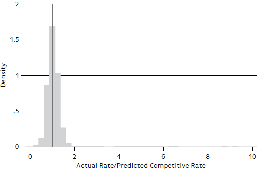
FIGURE B-1 Distribution of ratios of actual to predicted rates, nonbenchmark sample, farm products, no ratios excluded.
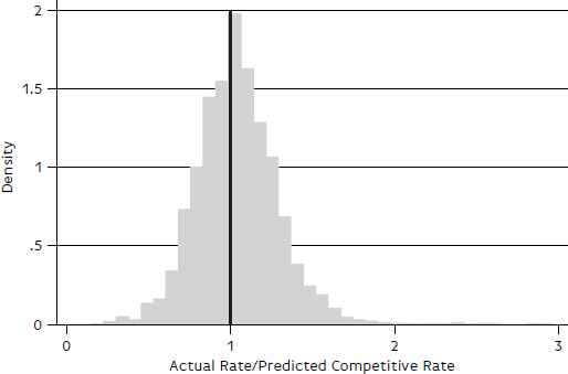
FIGURE B-2 Distribution of ratios of actual to predicted rates, nonbenchmark sample, farm products, ratios greater than 3 excluded.
TABLE B-3 Farm Products Model: Distribution of 2013 Test Group Observations, Ratios of Actual Rate to Benchmark Rate
| Group | Observations | Expanded | ||||||
| Contract No. | Tariff No. | Total | % | Cum. % | % | Cum. % | ||
| r ≤ 1 | 255 | 2,512 | 2,767 | 43.2 | 43.2 | 41.7 | 41.7 | |
| 1 < r ≤ 1.2 | 96 | 1,971 | 2,067 | 32.3 | 75.5 | 31.4 | 73.1 | |
| 1.2 < r ≤ 1.4 | 25 | 1,017 | 1,042 | 16.3 | 91.8 | 16.3 | 89.4 | |
| 1.4 < r ≤ 1.6 | 1 | 299 | 300 | 4.7 | 96.5 | 6.6 | 96 | |
| 1.6 < r ≤ 1.8 | 1 | 72 | 73 | 1.1 | 97.7 | 1.3 | 97.3 | |
| 1.8 < r ≤ 2.0 | 0 | 22 | 22 | 0.3 | 98.0 | 0.6 | 97.9 | |
| r > 2.0 | 5 | 123 | 128 | 2.0 | 100 | 2.1 | 100 | |
| Total | 383 | 6,016 | 6,399 | 100 | 100 | |||
NOTE: The groups are defined by the ratio (r) of actual revenue per ton-mile (ARTM) to the predicted 50th percentile. Cum. = cumulative. The columns showing expanded percentages use the sample rate expansion factor associated with each observation.
of shipments. Because this finding holds across all four models, it is not repeated.
Coal
The descriptive statistics for coal are provided in Table B-4. There are 446,820 total observations, with 291,431 in the competitive benchmark sample and 155,389 in the nonbenchmark sample. The benchmark sample rates are lower on average (3.4 cents versus 4.2 cents per ton-mile), shipment distances are longer (721 versus 473 miles), and shipment sizes are greater (82 versus 24 cars). Water is a less likely competitive option for the benchmark group, since 36 percent of the observations have no water access within 50 miles, compared with 16 percent of the
TABLE B-4 Coal Summary Statistics, 2000–2013
| Variable | Combined Samples | Benchmark Sample | Nonbenchmark Sample |
| Observations | 446,820 | 291,431 | 155,389 |
| Revenue per ton-mile (2009 dollars) | 0.039 | 0.034 | 0.042 |
| Distance (miles) | 569 | 721 | 473 |
| Shipment size (number of cars) | 46 | 82 | 24 |
| Number of railroads in shipment | 1.19 | 1.30 | 1.16 |
| Number of Class I railroads within 10 miles of origin | 1.84 | 1.91 | 1.80 |
| Number of Class I railroads within 10 miles of destination | 2.52 | 2.72 | 2.40 |
| No water ports within 50 miles (binary) | 0.24 | 0.36 | 0.16 |
| Distance to water from origin (miles) | 202 | 304 | 137 |
| Distance to water from destination (miles) | 67 | 89 | 53 |
| Private car (binary) | 0.37 | 0.58 | 0.23 |
NOTE: All values are means weighted by the expansion factor associated with each sampled shipment.
nonbenchmark group. Furthermore, the distances to water are higher for the benchmark group—304 miles from the origin and 89 miles from the destination versus 137 miles and 53 miles, respectively, for the nonbenchmark group. Finally, the percentage of private cars is much higher for the benchmark group (58 versus 23 percent).
The regression results are shown in Table B-5. The coal model was developed with a binary variable (West), which was set at 1 for shipments originating west of the Mississippi River. This variable was added to account for western coal shipments typically being much larger and moving longer distances than eastern coal shipments and because western coal has lower sulfur content than eastern coal, which makes them somewhat different products. Again, the intercept effects (rail, STCC level 5, and annual dummies) are suppressed. As in the case of farm products, the signs of the coefficients are consistent across columns, and the results are stable across columns in terms of the magnitudes of the coefficient estimates. As might be expected, longer shipment distances and larger shipment sizes tend to predict lower rates (revenue per ton-mile). One anomaly is the number of railroads involved in the shipment. In some specifications this coefficient is negative, while in other specifications it is positive. However, for nearly 90 percent of the observations, one railroad is involved in the shipment. Rail competition at the origin or destination predicts lower prices in all specifications. The presence of water competition and shorter distances to water from the origin and destination both predict lower rates, while the use of private cars predicts lower rates. Western coal tends to have lower rates, all else equal, than eastern coal.
As before, the results in Table B-5 for the 50th percentile (median) are used to predict the rates for the 3,670 observations in the 2013 test group. The ratio of the actual rate to the predicted rate is summarized in Figure B-3 and Figure B-4 and in Table B-6. Most of the observations are clustered around 1, but some values exceed 3.
Chemicals
The descriptive statistics for chemicals for 2000 through 2013 are provided in Table B-7. There are 556,467 total observations, with 357,998
TABLE B-5 Benchmark Models: Coal
| Quantile | |||||
| Variable | OLS | 0.25 | 0.5 | 0.75 | 0.9 |
| ln(distance) | −0.436 (0.00201) | −0.362 (0.00132) | −0.446 (0.00128) | −0.510 (0.00148) | −0.527 (0.000850) |
| ln(cars) | −0.114 (0.00153) | −0.111 (0.000684) | −0.112 (0.000634) | −0.113 (0.000701) | −0.103 (0.000821) |
| ln(number of railroads) | −0.0703 (0.00619) | −0.0994 (0.00319) | −0.0871 (0.00409) | 0.135 (0.00437) | 0.213 (0.00504) |
| No. of Class I within 10 mi of origin | −0.0899 (0.00104) | −0.0807 (0.000464) | −0.0965 (0.000541) | −0.101 (0.00109) | −0.0952 (0.00136) |
| No. of Class I within 10 mi of destination | −0.0468 (0.000902) | −0.0481 (0.000616) | −0.0521 (0.000689) | −0.0429 (0.000653) | −0.0418 (0.000644) |
| West (binary) | −0.265 (0.00833) | −0.346 (0.00430) | −0.235 (0.0114) | −0.0335 (0.00459) | −0.0400 (0.00988) |
| Nowater (binary) | 0.204 (0.00901) | 0.166 (0.00425) | 0.203 (0.00427) | 0.273 (0.00556) | 0.160 (0.00706) |
| ln(mi from origin to port) | 0.0299 (0.00145) | 0.0235 (0.000901) | 0.0275 (0.000657) | 0.0414 (0.000977) | 0.0112 (0.00125) |
| ln(mi from destination to port) | 0.0257 (0.000825) | 0.0279 (0.000679) | 0.0280 (0.000453) | 0.0290 (0.000692) | 0.0249 (0.000607) |
| Private car (binary) | −0.124 (0.00297) | −0.115 (0.00204) | −0.104 (0.00213) | −0.0671 (0.00208) | −0.107 (0.00206) |
| Observations | 289,718 | 289,718 | 289,718 | 289,718 | 289,718 |
| R2 | 0.785 | ||||
NOTE: Based on competitive benchmark data. All standard errors are p < .01. All results are weighted by the expansion factor.
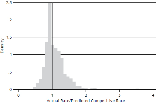
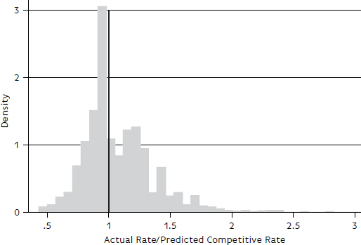
TABLE B-6 Coal Model: Distribution of 2013 Test Group Observations, Ratios of Actual Rate to Benchmark Rate
| Observations | Expanded | |||||||
| Group | Contract No. | Tariff No. | Total | % | Cum. % | % | Cum. % | |
| r ≤ 1 | 679 | 1,175 | 1,854 | 50.5 | 50.5 | 54.7 | 54.7 | |
| 1 < r ≤ 1.2 | 85 | 657 | 742 | 20.2 | 70.7 | 20.1 | 74.9 | |
| 1.2 < r ≤ 1.4 | 167 | 412 | 579 | 15.8 | 86.5 | 12.9 | 87.7 | |
| 1.4 < r ≤ 1.6 | 77 | 213 | 290 | 7.9 | 94.4 | 6.9 | 94.6 | |
| 1.6 < r ≤ 1.8 | 61 | 50 | 111 | 3.0 | 97.4 | 2.5 | 97.1 | |
| 1.8 < r ≤ 2.0 | 13 | 24 | 37 | 1.0 | 98.4 | 1.1 | 98.2 | |
| r > 2.0 | 10 | 47 | 57 | 1.6 | 100 | 1.8 | 100 | |
| Total | 1,092 | 2,578 | 3,670 | 100 | 100 | |||
NOTE: The groups are defined by the ratio (r) of ARTM to the predicted 50th percentile. Cum. = cumulative. The columns showing expanded percentages use the sample rate expansion factor associated with each observation.
in the competitive benchmark group and 198,469 in the nonbenchmark group. In 2009 dollars, the average rate for the combined sample is 8.6 cents per ton-mile. The average distance traveled is 778 miles, and the average shipment size is 1.2 cars. Most shipments involve only one railroad, and shippers have on average 2.6 railroads within 10 miles of the origin and 2.5 railroads within 10 miles of the destination. About 20 percent of shipments have no water options within 50 miles. Finally, about 96 percent of movements are made in private cars, since railroads own few tank cars. There is little difference across the two groups for most variables. However, the nonbenchmark shipments tend to have less access to rail and water.
In the chemical specification, a dummy variable is added to denote hazardous materials in recognition of potential added costs associated with transporting hazardous chemicals. About 38 percent of the shipments are hazardous materials. The estimation results are summarized
TABLE B-7 Chemicals Summary Statistics, 2000–2013
| Variable | Combined Samples | Benchmark Sample | Nonbenchmark Sample |
| Observations | 556,467 | 357,998 | 198,469 |
| Average revenue per ton-mile (2009 dollars) | 0.086 | 0.090 | 0.082 |
| Distance (miles) | 778 | 757 | 815 |
| Shipment size (number of cars) | 1.20 | 1.20 | 1.21 |
| Number of railroads in shipment | 1.30 | 1.31 | 1.28 |
| Number of Class I railroads within 10 miles of origin | 2.59 | 2.79 | 2.23 |
| Number of Class I railroads within 10 miles of destination | 2.54 | 2.59 | 2.44 |
| No water ports within 50 miles (binary) | 0.20 | 0.16 | 0.27 |
| Distance to water from origin (miles) | 95 | 76 | 129 |
| Distance to water from destination (miles) | 94 | 86 | 109 |
| Private car (binary) | 0.96 | 0.97 | 0.94 |
NOTE: All values are means weighted by the expansion factor associated with each sampled shipment.
in Table B-8, excluding all fixed effects. The coefficient estimates for the same variable have the same sign across table columns. The magnitudes are also stable across columns. Increasing shipment distance and size both predict lower rates (revenue per ton-mile), while an increase in the number of railroads involved in the move predicts higher rates. The competition variables for both rail and water are statistically important and have signs that are consistent with the cited literature.
The median regression (quantile = 0.5) results in Table B-8 are again used to predict the rates for the 2013 test group, which totaled 8,176 observations. The ratios of actual to predicted rates are summarized in Figure B-5 and Figure B-6 and in Table B-9. As shown in Figure B-5, the distribution is positively skewed, with some very large
TABLE B-8 Benchmark Models: Chemicals
| Quantile | |||||
| Variable | OLS | 0.25 | 0.5 | 0.75 | 0.9 |
| ln(distance) | −0.537 (0.00106) | −0.478 (0.00105) | −0.526 (0.00115) | −0.576 (0.00100) | −0.611 (0.00134) |
| ln(cars) | −0.0674 (0.00133) | −0.0584 (0.000811) | −0.0643 (0.00108) | −0.0682 (0.00123) | −0.0705 (0.000964) |
| ln(number of railroads) | 0.314 (0.00307) | 0.248 (0.00246) | 0.269 (0.00256) | 0.294 (0.00253) | 0.350 (0.00385) |
| No. of Class I within 10 mi of origin | −0.0093 (0.000603) | −0.0204 (0.000452) | −0.0233 (0.000580) | −0.0171 (0.000563) | −0.0076 (0.000718) |
| No. of Class I within 10 mi of destination | −0.0521 (0.000607) | −0.0609 (0.000557) | −0.0570 (0.000665) | −0.0470 (0.000649) | −0.0362 (0.000517) |
| Nowater (binary) | 0.0564 (0.00364) | 0.0739 (0.00300) | 0.0687 (0.00371) | 0.0614 (0.00356) | 0.0333 (0.00419) |
| ln(mi from origin to port) | 0.00864 (0.000572) | 0.00947 (0.000484) | 0.00963 (0.000586) | 0.00653 (0.000557) | 0.00285 (0.000617) |
| ln(mi from destination to port) | 0.0146 (0.000574) | 0.0194 (0.000521) | 0.0189 (0.000612) | 0.0168 (0.000579) | 0.0135 (0.000649) |
| Private car (binary) | −0.102 (0.00437) | −0.115 (0.00320) | −0.0940 (0.00411) | −0.0817 (0.00350) | −0.0924 (0.00465) |
| Hazmat (binary) | 0.0708 (0.00273) | 0.0434 (0.00203) | 0.0701 (0.00244) | 0.0666 (0.00258) | 0.0511 (0.00295) |
| Observations | 356,187 | 356,187 | 356,187 | 356,187 | 356,187 |
| R2 | 0.656 | ||||
NOTE: Based on competitive benchmark data. All standard errors are p < .01. All results are weighted by the expansion factor

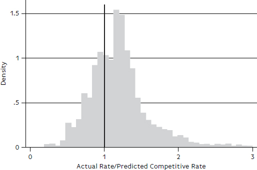
TABLE B-9 Chemicals Model: Distribution of 2013 Test Group Observations, Ratios of Actual Rate to Benchmark Rate
| Observations | Expanded | |||||||
| Group | Contract No. | Tariff No. | Total | % | Cumulative % | % | Cumulative % | |
| r ≤ 1 | 521 | 1,991 | 2,512 | 30.7 | 30.7 | 33.0 | 33.0 | |
| 1 < r ≤ 1.2 | 187 | 1,719 | 1,906 | 23.3 | 54.0 | 24.1 | 57.1 | |
| 1.2 < r ≤ 1.4 | 108 | 1,774 | 1,882 | 23.0 | 77.1 | 21.4 | 78.5 | |
| 1.4 < r ≤ 1.6 | 71 | 658 | 729 | 8.9 | 86.0 | 7.7 | 86.2 | |
| 1.6 < r ≤ 1.8 | 60 | 328 | 388 | 4.7 | 90.7 | 4.4 | 90.6 | |
| 1.8 < r ≤ 2.0 | 44 | 223 | 267 | 3.3 | 94.0 | 3.1 | 93.7 | |
| r > 2.0 | 26 | 466 | 492 | 6.0 | 100 | 6.3 | 100 | |
| Total | 1,017 | 7,159 | 8,176 | 100 | 100 | |||
NOTE: The groups are defined by the ratio (r) of ARTM to the predicted 50th percentile. The columns showing expanded percentages use the sample rate expansion factor associated with each observation.
values. The maximum ratio is 19.8. As noted earlier, this large dispersion (compared with the other models), with more than 6 percent of observations having ratios greater than 2, may stem from the variability in the types of chemical products and their associated shipping characteristics. A more refined chemical model based on product may be warranted.
Petroleum
The descriptive statistics for petroleum for 2000–2013 are provided in Table B-10. There are 86,678 total observations, with 50,487 in the competitive benchmark group and 36,191 in the nonbenchmark group. In 2009 dollars, the average price for the combined sample is 9.9 cents per ton-mile. The average distance traveled is 793 miles, and the average shipment size is 1.1 cars. Most shipments involve only one
TABLE B-10 Petroleum Summary Statistics, 2000–2013
| Variable | Combined Samples | Benchmark Sample | Nonbenchmark Sample |
| Observations | 86,678 | 50,487 | 36,191 |
| Average revenue per ton-mile (2009 dollars) | 0.099 | 0.095 | 0.104 |
| Distance (miles) | 793 | 786 | 804 |
| Shipment size (number of cars) | 1.10 | 1.09 | 1.12 |
| Number of railroads in shipment | 1.31 | 1.34 | 1.28 |
| Number of Class I railroads within 10 miles of origin | 2.50 | 2.70 | 2.21 |
| Number of Class I railroads within 10 miles of destination | 2.37 | 2.48 | 2.20 |
| No water ports within 50 miles (binary) | 0.15 | 0.09 | 0.23 |
| Distance to water from origin (miles) | 92 | 64 | 131 |
| Distance to water from destination (miles) | 92 | 76 | 113 |
| Private car (binary) | 0.99 | 0.99 | 0.99 |
NOTE: All values are means weighted by the expansion factor associated with each sampled shipment.
railroad, and shippers on average have 2.5 railroads within 10 miles of the origin and 2.4 railroads within 10 miles of the destination. About 15 percent of total shipments have no water options within 50 miles, but the benchmark shippers have more access, with only about 9 percent having no water options; the nonbenchmark shippers are somewhat more restricted in their water options (about 23 percent have no water options). Finally, virtually all movements occur in private cars because railroads own very few tank cars. There is little difference across the two samples in most variables other than the water options and the distance to water for both origins and destinations.
The estimation results are summarized in Table B-11 with the intercept effects (railroad dummies, annual dummies, and STCC
TABLE B-11 Benchmark Models: Petroleum and Products
| Quantile | |||||
| Variable | OLS | 0.25 | 0.5 | 0.75 | 0.9 |
| ln(distance) | −0.617 (0.00247) | −0.553 (0.00229) | −0.606 (0.00236) | −0.638 (0.00230) | −0.668 (0.00274) |
| ln(cars) | 0.0196 (0.00470) | 0.0311 (0.00478) | 0.00899** (0.00366) | −0.00350 (0.00402) | −0.0115 (0.00275) |
| ln(number of railroads) | 0.358 (0.00680) | 0.326 (0.00498) | 0.308 (0.00502) | 0.326 (0.00563) | 0.424 (0.00796) |
| No. of Class I within 10 mi of origin | 0.00518 (0.00158) | −0.0165 (0.00147) | −0.0137 (0.00148) | 0.00330** (0.00149) | 0.0273 (0.00216) |
| No. of Class I within 10 mi of destination | −0.0569 (0.00161) | −0.0624 (0.00119) | −0.0671 (0.00139) | −0.0515 (0.00156) | −0.0344 (0.00214) |
| Nowater (binary) | 0.113 (0.00784) | 0.0965 (0.00654) | 0.0759 (0.00880) | 0.0513 (0.00728) | 0.0181** (0.00843) |
| ln(mi from origin to port) | 0.00669 (0.00116) | 0.00492 (0.00115) | 0.00698 (0.00113) | 0.00120 (0.00103) | −0.00727 (0.00143) |
| ln(mi from destination to port) | 0.0127 (0.00118) | 0.0155 (0.00121) | 0.0106 (0.00108) | 0.00278** (0.00109) | 0.00336** (0.00145) |
| Private car | 0.0863* (0.0509) | −0.180 (0.0204) | 0.000810 (0.0153) | 0.134 (0.0768) | 0.0414 (0.125) |
| Observations | 50,340 | 50,340 | 50,340 | 50,340 | 50,340 |
| R2 | 0.749 | ||||
NOTE: Based on competitive benchmark data. All standard errors are p < .01, except ** = p < .05 and * = p < .1. All results are weighted by the expansion factor.
dummies) suppressed. In general, the coefficient estimates for the same variable have the same sign across columns of the table for most of the variables (i.e., distance, number of railroads in the movement, the number of Class I carriers within 10 miles of the destination, the presence of water, and the distance to water from the destination). However, there are some differences. They include shipment size, the
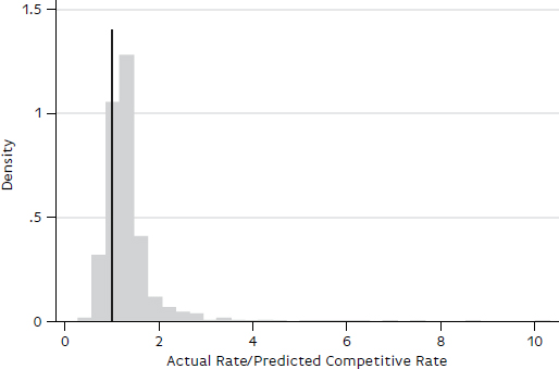
FIGURE B-7 Distribution of ratios of actual to predicted rates, nonbenchmark sample, petroleum, no ratios excluded.
number of Class I railroads within 10 miles of the origin, and the distance to water from the origin.
As with the other models, the median regression (quantile = 0.5) results in Table B-11 are used to predict the rates for the 2,670 observations in the test group. The ratios of actual to predicted rates are summarized in Figures B-7 and B-8 and in Table B-12. As shown in Figure B-7, the distribution is positively skewed, with some very large values. The maximum ratio is 10.31. However, most of the ratios are between 0 and 2, as shown in Figure B-8 and Table B-12.
CONCLUSIONS
Railroads are subject to maximum rate regulation intended to allow the railroads to earn revenues adequate to cover their common costs while protecting shippers with few competitive options from unreasonably high common carrier rates. A major problem for regulators has been
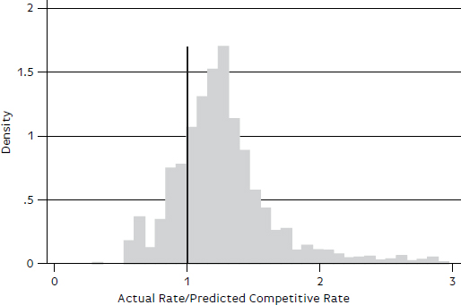
FIGURE B-8 Distribution of ratios of actual to predicted rates, nonbenchmark sample, petroleum, ratios greater than 3 excluded.
TABLE B-12 Petroleum Model: Distribution of 2013 Test Group Observations, Ratios of Actual Rate to Benchmark Rate
| Observations | Expanded | |||||||
| Group | Contract No. | Tariff No. | Total | % | Cumulative % | % | Cumulative % | |
| r ≤ 1 | 117 | 418 | 535 | 20.0 | 20.0 | 19.3 | 19.3 | |
| 1 < r ≤ 1.2 | 4 | 665 | 669 | 25.1 | 45.1 | 24.9 | 44.3 | |
| 1.2 < r ≤ 1.4 | 9 | 724 | 733 | 27.5 | 72.5 | 27.6 | 71.9 | |
| 1.4 < r ≤ 1.6 | 6 | 354 | 360 | 13.5 | 86.0 | 13.8 | 85.7 | |
| 1.6 < r ≤ 1.8 | 0 | 137 | 137 | 5.1 | 91.2 | 5.3 | 91.0 | |
| 1.8 < r ≤ 2.0 | 10 | 43 | 53 | 2.0 | 93.1 | 2.0 | 93.0 | |
| r > 2.0 | 9 | 174 | 183 | 6.9 | 100 | 7.0 | 100 | |
| Total | 155 | 2,515 | 2,670 | 100 | 100 | |||
NOTE: The groups are defined by the ratio (r) of ARTM to the predicted 50th percentile. The columns showing expanded percentages use the sample rate expansion factor associated with each observation.
in determining whether a particular rate is high enough to warrant additional regulatory scrutiny. The current system uses a threshold of 180 percent of the Uniform Railroad Costing System–estimated average “variable cost” for this purpose, which is unreliable and arbitrary, as documented in this report.
An alternative approach for identifying unusually high rates is demonstrated in this appendix. The concept is that some shipments whose rates are determined under competitive conditions can be used to estimate competitive benchmark prices for other shipments with varying degrees of competition and cost-related characteristics. The method was demonstrated for movements of farm products, coal, chemicals, and petroleum. In general, the predictive models of the price of an effectively competitive movement given the route characteristics perform well in explaining the data. For the most part, the tested rates were close to the competitive rates, but the procedure identifies traffic having rates that far exceed the competitive benchmark rate. These rates might be candidates for further scrutiny for reasonableness.
REFERENCES
Barnekov, C. C., and A. N. Kleit. 1990. The Efficiency Effects of Railroad Deregulation in the United States. International Journal of Transport Economics, Vol. 17, No. 1, pp. 21–36.
Boyer, K. D. 1987. The Cost of Price Regulation: Lessons from Railroad Deregulation. Rand Journal of Economics, Vol. 18, No. 3, pp. 408–416.
Burton, M. L. 1993. Railroad Deregulation, Carrier Behavior, and Shipper Response: A Disaggregated Analysis. Journal of Regulatory Economics, Vol. 5, No. 4, pp. 417–434.
Burton, M. L., and W. W. Wilson. 2006. Network Pricing: Service Differentials, Scale Economies, and Vertical Exclusion in Railroad Markets. Journal of Transport Economics and Policy, Vol. 40, No. 2, pp. 255–277.
Dennis, S. M. 2000. Changes in Railroad Rates Since the Staggers Act. Transportation Research Part E, Vol. 37, pp. 55–69.
Grimm, C. M., C. Winston, and C. A. Evans. 1992. Foreclosure of Railroad Markets: A Test of Chicago Leverage Theory. Journal of Law and Economics, Vol. 35, No. 2, Oct., pp. 295–310.
Koenker, R., and G. Bassett. 1982. Regression Quantiles. Econometrica, Vol. 46, No. 1, pp. 33–50.
MacDonald, J. M. 1987. Competition and Rail Rates for the Shipment of Corn, Soybeans, and Wheat. Rand Journal of Economics, Vol. 18, No. 1, pp. 151–163.
MacDonald, J. M. 1989. Railroad Deregulation, Innovation, and Competition: Effects of the Staggers Act on Grain Transportation. Journal of Law and Economics, Vol. 32, pp. 63–96.
McFarland, H. 1989. The Effects of United States Railroad Deregulation on Shippers, Labor, and Capital. Journal of Regulatory Economics, Vol. 1, pp. 259–270.
Schmidt, S. 2001. Market Structure and Market Outcomes in Deregulated Rail Freight Markets. International Journal of Industrial Economics, Vol. 19, Nos. 1–2, pp. 99–131.
Silverman, B. W. 1986. Density Estimation for Statistics and Data Analysis. Chapman and Hall.
Wilson, W. W. 1994. Market-Specific Effects of Rail Deregulation. Journal of Industrial Economics, Vol. 42, No. 1, pp. 1–22.


