
![]()
Role of the Inland Waterways System in National Freight Transportation
This chapter describes the inland waterways, with a focus on those parts used to transport freight and an eye toward describing certain aspects of the system that warrant consideration in decisions about funding. The first section below describes the physical characteristics and history of the system. The next describes the major corridors, the commodities shipped, and the contribution of the inland waterways system to national freight transportation relative to other modes. The condition and performance of the system, including reliability (delays and unavailabilities), usage, and age of the infrastructure, are then discussed. An alternative approach for assessing the age of infrastructure is considered, and a model and possible metrics for understanding the impact of delays across the system are offered. The final section summarizes findings and conclusions from the chapter.
Overview of U.S. Inland Waterways
CHARACTERISTICS
The inland waterways navigation system is part of the U.S. marine transportation system (MTS), which provides for both passenger transport and domestic freight transportation infrastructure and coastal gateways for global trade (TRB 2004). The MTS includes navigable waterways and public and private ports on three coasts (Atlantic, Pacific, and Gulf) and the Great Lakes as well as a network of inland waterways (CMTS 2008). It includes, by extension, inland highway and rail connections between ports and inland markets that ensure access to the water for shippers and customers in all 50 states (AASHTO 2013; CMTS 2008).
The inland and intracoastal waterways directly serve 41 states1 (Clark et al. 2012).
The inland waterways system comprises navigable rivers linked by a series of major canals. Lock and dam infrastructure is the chief mechanism in enabling the upstream and downstream movement of cargo, and its installation is the most expensive component in providing for navigation service (McCartney et al. 1998).2 Waterways are categorized as deep draft, shallow draft, both (allowing both shallow and deep draft vessels), or nonnavigable, as shown in Table 2-1, which reports the average control depths in the U.S. Army Corps of Engineers (USACE) geographic information system (GIS) data. Because of shallow drafts and seasonal changes in navigable depths, fixed infrastructure is required in many parts of the river system to maintain open navigation for commerce.
The nation’s inland waterways include more than 36,000 miles of rivers, waterways, channels, and canals, with 241 locks managed by USACE at 195 sites.3 [Kruse et al. 2007; USACE Navigation Data
________________
1 The U.S. Army Corps of Engineers geographic information system viewer data can mostly confirm this. The committee counts 39 states (40 including the District of Columbia) if the focus is on shallow draft or both shallow and deep draft and if nonnavigable and deep draft (only) and unknown segments are eliminated. Some of the inland and intracoastal waterways are access routes for deep draft vessels; with those included, the committee counts 41 (43 including the District of Columbia and Puerto Rico). Some are coastal states (e.g., California, Delaware, New Jersey, Maryland) with minor inland or intracoastal waterways outside of the committee’s charter. For example, 12 states, ranked by ton-miles, account for 80 percent of ton-miles and 74 percent of tons moved by inland waterway. Conversely, an overlapping but not identical 12 states ranked by tons account for 80 percent of the tons and 75 percent of the ton-miles moved by inland waterway.
2 The U.S. Army Corps of Engineers Navigation Data Center provides data on the national waterways network with defined geographic classes that include ocean, Great Lakes, and inland rivers (http://www.navigationdatacenter.us/data/dictionary/ddnwn.htm).
3 The USACE GIS viewer data identify some 250 locks in the USACE Navigation Data Center GIS data. Nineteen are listed as seasonal. The analysis in this chapter eliminated those identified as caretaker, closed, or inoperable.
Included in the 36,000 miles are the Erie Canal, a portion of the Saint Lawrence Seaway (the 101.2-mile stretch that borders New York from Lake Ontario), and other border connections such as Lake of the Woods to Lake Superior and the Saint Marys River connecting Lakes Superior and Huron. The full extents of the Gulf Intracoastal and Atlantic Intracoastal Waterways are also included.
Navigable waterways are defined in terms of the USACE link data dictionary (http://www.navigationdatacenter.us/data/dictionary/ddnwn.htm) in the GIS data set nwn.zip available at http://www.navigationdatacenter.us/db/gisviewer/, with GEO = I, inland, for the contiguous United States.
TABLE 2-1 Summary Characteristics of the Inland Waterways of the National Waterways Network
| Inland Geographic Class | Length of Waterway (miles) | Average Control Depth (feet) |
| Deep draft navigation | 1,901 | 35 |
| Shallow draft navigation | 21,218 | 10 |
| Both (deep and shallow draft) | 13,205 | 28 |
| Total | 36,324 | |
NOTE: Shallow draft navigation includes all waterway segments with navigable depths; not all of these waterways carry substantial cargo. About 11,000 of the 36,000 inland waterway miles are part of the fuel-taxed inland waterways navigation system specified in legislation and subject to a barge fuel tax used to pay 50 percent of the costs of inland waterways system infrastructure construction (see Appendix A for a list of fuel-taxed inland waterways).
SOURCE: USACE Navigation Data Center GIS Viewer (http://www.navigationdatacenter.us/db/gisviewer, file ndcgis13shp.zip, updated May 16, 2013; accessed July 2014).
Center GIS Viewer files (http://www.navigationdatacenter.us/db/gisviewer, accessed July 2014)]. As shown in Figure 2-1, most of the navigable channels are rivers located in the central and eastern half of the country. The largest river system is the Mississippi, which is navigable for about 1,800 miles from New Orleans, Louisiana, to Minneapolis, Minnesota, and has a large tributary system. In the western part of the country the largest inland waterway is the Columbia–Snake River system. As described in Chapter 1, this report covers the inland waterways, excluding the Saint Lawrence Seaway system and the Great Lakes.
HISTORICAL CONTEXT
At the time of the American Revolution (1775–1783), a shipper had to pay as much to move a ton of freight 30 miles inland as to move it across the Atlantic (AASHTO 2013). As the new nation
________________
USACE has responsibility for enabling commercial navigation on approximately 25,000 of these miles. [See the nwn.zip (http://www.navigationdatacenter.us/db/gisviewer/) data set filtered by GEO = I, inland; FUNC = S, D, B; WTYPE = 2, 6–9, 12 for all states in the contiguous United States; see the USACE link data dictionary (http://www.navigationdatacenter.us/data/dictionary/ddnwn.htm) for a complete description of the codes used. All data sets were accessed in September 2014.]
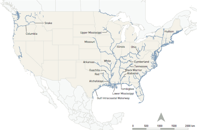
FIGURE 2-1 Inland and intracoastal waterways system.
SOURCE: USACE Navigation Data Center GIS Viewer (http://www.navigationdatacenter.us/db/gisviewer, file ndcgis13shp.zip, updated May 16, 2013; accessed July 2014).
began building, leaders understood that a good transportation system would be essential in opening the country’s vast interior and increasing national wealth. In view of the availability of easily navigable waterways, waterborne commerce was the primary viable option for transporting freight over significant distances. The inland waterways carried grain, lumber, and coal to the eastern ports and finished goods and immigrants to the rapidly developing Northwest Territory (National Park Service 2013).
The emergence and rapid expansion of railroads complemented the north–south river system with an east–west alignment. Railroads allowed waterways to become even more productive as they carried goods to river ports, where they were consolidated and moved by barge to seaports for export (AASHTO 2013). Later, rail became a direct substitute for slower canal transport. In the early 20th century, the development of technologies related to automobiles, trucks, and highways spurred a new age of industrial development in the United States (AASHTO 2013). Trucking emerged as the most viable mode for serving local and regional freight markets. Trucks carried water and rail freight to and from the interior communities and functioned as a faster door-to-door mode for higher-value cargoes. The federal Interstate and state highway networks made trucking competitive with rail serving long-haul markets for time-sensitive, high-value commodities with speedy, reliable service (AASHTO 2013). Intermodal freight systems became the standard for non-bulk products with the introduction of containerization, unitized cargo configurations that could be transferred among truck, rail, and water modes without repackaging. Associated technologies made their tracking and reliable delivery more transparent to shippers.
NATIONAL ECONOMY
The inland waterways freight system makes a relatively small but stable contribution to the overall economy. Since 2000, it has carried about half of domestic U.S. waterborne commerce, measured in ton-miles, and 6 to 7 percent of all ton-miles (Figure 2-2).
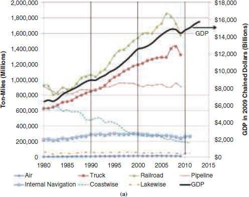
FIGURE 2-2 Trends for various modes in terms of (a) ton-miles and (b, next page) U.S. GDP. These data do not include trends in foreign imports of cargo delivered to U.S. ports. That is, imports become domestic after processing through U.S. Customs at ports of entry; therefore, trucking volumes and some rail volumes increase over time because of growth in imported freight flows, whereas U.S. pipeline transport and domestic waterway transport primarily serve domestic-only freight flows (with the notable exception of grain exports).
SOURCE: GDP is from the Bureau of Economic Analysis, current-dollar and “real” GDP (http://www.bea.gov/national/xls/gdplev.xls, accessed May 29, 2014), where GDP is in billions of chained 2009 dollars; ton-miles data were compiled from the National Transportation Statistics of the Bureau of Transportation Statistics, various years (http://www.rita.dot.gov/bts/sites/rita.dot.gov.bts/files/publications/national_transportation_statistics/html/table_01_50.html and http://www.rita.dot.gov/bts/node/81022, accessed May 2014).
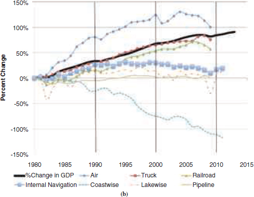
FIGURE 2-2 Trends for various modes in terms of (b) U.S. GDP.
Some modes of transportation are correlated with the economy measured in terms of gross domestic product (GDP), especially truck and rail, which deliver goods for final consumption. Other modes are less correlated with economic growth, such as waterborne commerce and pipeline transportation of energy products. Pipelines and barge are more specialized modes that carry a narrower range of products than trucking or rail and may be correlated with the output of the industries whose goods they carry. These modes provide essential transportation services that underpin the ability of trucking and rail to deliver consumer products.
The following will help put in perspective the contribution of waterborne commerce to the U.S. economy. The transportation sector overall contributes approximately 3 percent of U.S. GDP, according to the Bureau of Economic Analysis (http://www.bea.gov/iTable
/index_industry_gdpIndy.cfm). Water transportation contributes nearly $15 billion in value added to U.S. GDP, compared with nearly $120 billion from truck transportation, more than $60 billion from air transportation, more than $30 billion from rail transportation, and $15 billion from pipeline transportation (Table 1 in http://www.bea.gov/scb/pdf/2012/05%20May/0512_industry.pdf and Table 1-2 in the North American Transportation Statistics, http://nats.sct.gob.mx/en/). Water transportation represents about 0.1 percent of total GDP. This amount includes all water transportation for passengers and freight, since data are not available specific to the inland waterways and freight. As shown in Figure 2-3, the transport sector contribution to GDP is declining (slightly), whereas water transport is about constant.
Similarly, the inland water transportation labor force has been constant for a number of years at about 20,000 (2007 census data, http://factfinder2.census.gov/faces/tableservices/jsf/pages/productview.xhtml?src=bkmk, and 2012 data from U.S. Census Bureau, 2012 County Business Patterns, accessed June 2014).
Freight traffic is highly variable across the inland waterways system, as shown in Figure 2-4. For the purpose of illustration, river segments are categorized in Figure 2-4 as high use, moderate use, or low use according to the number of ton-miles carried.4 Notably, the high-use parts of the inland waterways represent 22 percent of the total inland waterway miles and account for 76 percent of the cargo ton-miles transported5 (USACE 2013 and USACE Navigation Data Center, http://www.navigationdatacenter.us/db/gisviewer/, file linktons11.zip, updated August 14, 2013, and accessed July 2014).
________________
4 These category definitions for usage also form part of the guidance that USACE follows for spending priorities (USACE 2013, Appendix F, Table F-1 and Section F-12). The guidance allows for categorizing usage according to both number of ton-miles and number of lockages.
5 These percentages were computed by adding the ton-miles reported by the USACE Navigation Data Center within each illustrative usage category used by USACE and specified in the guidance (USACE 2013).
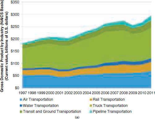
FIGURE 2-3 Summary of transportation contribution to U.S. GDP trends (a) in billions of dollars and (b, page 23) as a percentage of the total economy. Data show real dollars indexed to 2009. The data encompass all of water transportation, including passenger transportation; data are not available specific to the inland waterways and freight. Figures indicate the North American Industry Classification System categories. For further details, see http://nats.sct.gob.mx/english/go-to-tables/table-2-transportation-and-the-economy/table-2-1-gross-domestic-product-gdp-attributed-to-transportation-related-final-demand/#sthash.EenJZ015.dpuf.
SOURCE: NATS 2012, Table 2-1: Gross Domestic Product (GDP) Attributed to Transportation-Related Final Demand (http://nats.sct.gob.mx/english/go-to-tables/table-2-transportation-and-the-economy/table-2-1-gross-domestic-product-gdp-attributed-to-transportation-related-final-demand/, accessed July 2014).
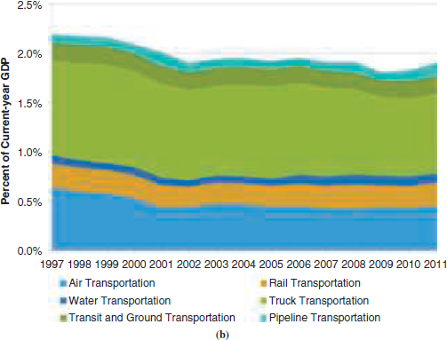
FIGURE 2-3 Summary of transportation contribution to U.S. GDP trends (b) as a percentage of the total economy.
Figure 2-4 also illustrates one of the thorny issues of inland waterways system funding. While some of the low-use tributaries appear to be less important, they may contribute shipments that join other commerce on the downstream moderate- and high-use segments. Since the shipments from individual low-use tributaries are a small contribution to total system flows, their marginal value added is also low, although their collective contribution is greater, and some individual segments may be important for moving cargo. When proponents of the inland waterways system refer to the need to preserve the network, they often are referring to these low-use tributaries and their contribution to total system freight flows. In many cases shippers have organized their operations to take advantage of low-cost water transportation of bulk commodities on these segments, and some would have few or no practical alternatives for shipping or receiving their bulk materials if the low-use segment were to be closed to commercial navigation.
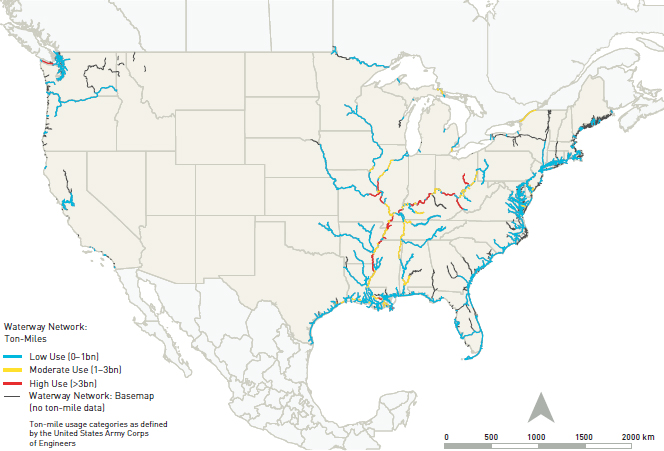
FIGURE 2-4 Inland waterways network with high-, moderate-, and low-use river segments in 2011.
SOURCE: USACE, Navigation Data Center, http://www.navigationdatacenter.us/db/gisviewer/, file linktons11.zip; updated August 14, 2013; accessed July 2014.
MAJOR INLAND WATERWAYS CORRIDORS
In 2012, inland waterways (internal) barge traffic accounted for 57 percent of U.S. domestic waterborne tonnage and about 70 percent of all domestic barge traffic (USACE 2013), as shown in Table 2-2.
Table 2-3 and the sections that follow summarize the features of the six major corridors that move substantial tonnages of waterborne commerce: the Upper Mississippi River, the Lower Mississippi River, the Ohio River, the Gulf Intracoastal Waterway (GIWW), the Illinois River, and the Columbia River system. This chapter focuses mainly on these six river corridors because they represent 80 percent of the commercial lockages, as shown later in Figure 2-13.6 For perspective, the miles of waterway on the six corridors represent about 16 percent of the total 36,000 inland river miles (as described in Table 2-1). These six rivers carry about 50 percent of the cargo transported (in ton-miles) on the inland waterways.7 While these six major corridors carry most of the freight, other river systems may transport regionally important commodities and may provide subcorridor routes for critically important freight movement at regional or national scales.8 (See Appendix B for a map representation and listing of major commodity-specific corridors generated from USACE Waterborne Commerce Statistics.)
Upper Mississippi River
The Upper Mississippi River flows south from Minneapolis, Minnesota, 858 miles to the mouth of the Ohio River at Cairo, Illinois. The navigation channel above Saint Louis, Missouri, is maintained at a minimum depth of 9 feet by a system of 27 locks and dams. As Table 2-3 indicates, agriculture-related products dominate the commodity flows on this river. Farm products, primarily grain shipped downbound for export through
________________
6 USACE Lock Use, Performance, and Characteristics, http://www.navigationdatacenter.us/lpms/lpms.htm, Locks by Waterway, Lock Usage, Calendar Years 1993–2013, accessed July 2014.
7 This statistic is derived from USACE commodity and usage statistics. Commodity statistics are at http://www.navigationdatacenter.us/lpms/cy2013comweb.htm. Usage statistics are at http://www.navigationdatacenter.us/lpms/lock2013web.htm.
8 Furthermore, the waterway freight tonnage data alone cannot fully characterize the economic value of the corridors because these freight flows necessarily involve drayage or long-haul trucking and can complement rail transport serving the commodities. For example, the heavy flow of coal by rail from the Powder River Basin to the Midwest is economically tied to the heavy waterway flows on the Mississippi and Ohio Rivers.
TABLE 2-2 Barge Freight Traffic Summary for 2012, by Commodity and Waterway Type
| Commodity | Total Barge | Coastwise or Lakewise | Inland (internal) | Intraport or Intraterritory | All Traffic (barge and nonbarge) | Barge (%) | Percent of All Domestic Traffic That Is Inland Barge (internal) | Percent of Barge Traffic That Is Inland Barge (internal) |
| Total | 737.6 | 101.1 | 557.6 | 79.1 | 884.8 | 83 | 63 | 76 |
| Coal | 182.7 | 4.0 | 169.0 | 9.7 | 200.0 | 91 | 85 | 93 |
| Petroleum and petroleum products | 252.4 | 55.5 | 149.2 | 47.7 | 311.1 | 81 | 48 | 59 |
| Chemicals and related products | 70.4 | 8.7 | 50.7 | 11.0 | 72.8 | 97 | 70 | 72 |
| Crude materials | 111.5 | 16.9 | 85.9 | 8.7 | 165.7 | 67 | 52 | 77 |
| Primary manufactured goods | 31.0 | 3.9 | 26.2 | 0.9 | 32.4 | 96 | 81 | 85 |
| Food and farm products | 76.1 | 1.9 | 73.7 | 0.5 | 79.1 | 96 | 93 | 97 |
| All manufactured equipment | 12.2 | 10.0 | 1.8 | 0.4 | 22.3 | 55 | 8 | 15 |
| Other | 1.3 | 0.0 | 1.0 | 0.3 | 1.5 | 100 | 67 | 77 |
NOTE: Except for percentages, figures are in millions of tons. “Intraport” refers to movement of freight within the confines of a port whether the port has one or several arms or channels included in the port definition. This traffic type will not include car ferries and general ferries moving within a port. “Intraterritory” refers to traffic between ports in Puerto Rico and the Virgin Islands, which are considered a single unit.
SOURCE: Table 2-3 of Part 5, National Summaries, Waterborne Commerce of the United States, 2012, published November 2013, http://www.navigationdatacenter.us/wcsc/wcsc.htm. (Values rounded to nearest 100,000 tons; therefore, percentages may differ because of rounding.)
TABLE 2-3 Freight Traffic for Six Major U.S. Inland Waterways, 2012
| Waterway Description | Commodities | Short Tons (millions) | Percent of Total | |
| Upper Mississippi River (Minneapolis, Minnesota, to mouth of Ohio River) | Total | 110.1 | 100 | |
| Coal | 24.1 | 21.9 | ||
| Petroleum and petroleum products | 12.8 | 11.6 | ||
| Chemicals and related products | 11.4 | 10.3 | ||
| Crude materials | 16.7 | 15.2 | ||
| Primary manufactured goods | 9.8 | 8.9 | ||
| Food and farm products | 35 | 31.7 | ||
| All manufactured equipment | 0.3 | 0.3 | ||
| Other | 0 | 0 | ||
| Lower Mississippi River (mouth of Ohio River to Baton Rouge, Louisiana) | Total | 186.3 | 100 | |
| Coal | 37.3 | 20 | ||
| Petroleum and petroleum products | 20.1 | 10.8 | ||
| Chemicals and related products | 22.3 | 11.9 | ||
| Crude materials | 31 | 16.6 | ||
| Primary manufactured goods | 12.8 | 6.9 | ||
| Food and farm products | 62.5 | 33.6 | ||
| All manufactured equipment | 0.4 | 0.22 | ||
| Other | 0 | 0 | ||
| Ohio River system | Total | 239.1 | 100 | |
| Coal | 140.2 | 58.5 | ||
| Petroleum and petroleum products | 14.4 | 6 | ||
| Chemicals and related products | 10.5 | 4.4 | ||
| Crude materials | 51.9 | 21.7 | ||
| Primary manufactured goods | 8.7 | 3.6 | ||
| Food and farm products | 13.4 | 5.6 | ||
| All manufactured equipment | 0.1 | 0.04 | ||
| Other | 0 | 0 | ||
| Waterway Description | Commodities | Short Tons (millions) | Percent of Total | |
| Gulf Intracoastal Waterway (from Florida to Texas) | Total | 113.7 | 100 | |
| Coal | 2.5 | 2.2 | ||
| Petroleum and petroleum products | 65.8 | 57.8 | ||
| Chemicals and related products | 21.2 | 18.7 | ||
| Crude materials | 16.7 | 14.7 | ||
| Primary manufactured goods | 4.6 | 4.1 | ||
| Food and farm products | 1.4 | 1.3 | ||
| All manufactured equipment | 0.8 | 0.7 | ||
| Other | 0.6 | 0.5 | ||
| Illinois River | Total | 31 | 100 | |
| Coal | 2.7 | 8.5 | ||
| Petroleum and petroleum products | 5.7 | 18.4 | ||
| Chemicals and related products | 5.2 | 16.7 | ||
| Crude materials | 3.2 | 10.4 | ||
| Primary manufactured goods | 3.6 | 11.6 | ||
| Food and farm products | 10.6 | 34.1 | ||
| All manufactured equipment | 0.1 | 0.24 | ||
| Other | 0 | 0 | ||
| Columbia River system (including Columbia, Willamette, and Snake Rivers) | Total | 57.3 | 100 | |
| Coal | 0 | 0 | ||
| Petroleum and petroleum products | 4.9 | 8.5 | ||
| Chemicals and related products | 6.1 | 10.6 | ||
| Waterway Description | Commodities | Short Tons (millions) | Percent of Total | |
| Columbia River system (continued) | Crude materials | 11.8 | 20.7 | |
| Primary manufactured goods | 2.6 | 4.5 | ||
| Food and farm products | 30.3 | 52.9 | ||
| All manufactured equipment | 0.9 | 1.7 | ||
| Other | 0.6 | 1.1 | ||
NOTE: These totals cannot be summed to compare with Table 2-2 because the same tonnages often move on connected rivers within commodity corridors; national summaries avoid duplicative reporting of total tonnages.
SOURCE: USACE, Waterborne Commerce of the United States, Calendar Year 2012, Waterborne Commerce Statistics Center, New Orleans, Louisiana, November 2013, Parts 2 and 4.
the Gulf Coast deepwater ports, account for 32 percent of the tonnage. The Upper Mississippi also is the top regional source for corn and soybean exports. The second-ranked commodity is coal, which accounts for 22 percent of the tonnage. Much of the chemical tonnage (10 percent of the total) consists of fertilizers shipped upbound back to the farm belt.
The dominant flows on the Upper Mississippi illustrate the modal competition and cooperation aspects of much waterborne commerce. For example, much of the grain is shipped by truck or rail to waterside grain elevators for transloading to barges, which then transload again to deepwater vessels in southern Louisiana for export to world grain markets. Trains also bring grain to the Gulf Coast, so for some farms there is at times a genuine modal choice between rail and water transport. However, grain transactions turn on margins as low as cents per bushel, so most shippers are essentially heavily dependent on one mode or the other. During the height of the harvest season, the capacities of both the rail and the inland waterways systems are stretched to keep up with shipping demand. The coal traffic on the system consists largely of low-sulfur coal that is shipped by unit train from the western coal fields to large
transloading facilities at places like Cora and Metropolis, Illinois, where it is loaded onto barges for movement to waterside electric power plants on the Ohio and Mississippi Rivers. Usually, competition among transport modes to serve a major shipper facility occurs when the facility site is being selected. Once the decision is made to locate a facility on a particular mode (e.g., a grain elevator or power plant is located on a river), goods movement tends to depend on that mode.
Lower Mississippi River
The Lower Mississippi River flows 956 miles from the mouth of the Ohio River at Cairo, Illinois, to the Mouth of Passes in the Gulf of Mexico. There are no navigation locks on this portion of the inland waterways system. Navigation depth is maintained by river training works such as groins and revetments and by periodic maintenance dredging of shoals. Operations on this segment typically feature large tows, since the size of tows is not constrained by lock sizes. Table 2-3 shows the commodity tonnages on the 720-mile stretch from Cairo to Baton Rouge, Louisiana. The commodity mix there is similar to that on the Upper Mississippi, but the quantities are 50 to 100 percent greater.
Ohio River System
The Ohio River begins at the junction of the Allegheny and Monongahela Rivers at Pittsburgh, Pennsylvania, and flows in a southwesterly direction 981 miles to its mouth at Cairo, Illinois, where it empties into the Mississippi River. Navigation is maintained at a minimum 9-foot channel depth by 20 locks and dams on the Ohio River (Olmsted Lock will replace two older locks near the lower end of the river). Table 2-3 shows the commodity flow on the entire Ohio River system, which includes the Ohio mainstem and its tributaries. The Monongahela, Kanawha, and Tennessee Rivers contribute significant flow to the Ohio.
Coal is the dominant commodity on the system, making up 59 percent of the tonnage in 2012. Most is steam coal, which moves both inbound and outbound on the system. Coal mines in Appalachia send coal to the river via conveyor belt, truck, and rail for shipment to river-located electric power generation plants. Those power plants also receive upbound coal from other sources, and there is still considerable movement of metallurgical coal on the Ohio and its tributaries. The
second-ranked commodity group, crude materials (nearly 22 percent of the total), consists primarily of sand, gravel, and limestone.
While rail lines run parallel along most of the Ohio, they are primarily part of the nation’s extensive east–west manufactured products and foodstuffs distribution system. As a practical matter, the large quantities of coal and crude materials moving on the Ohio could not easily be diverted to rail. Coal alone would require the railroads to handle more than 1 million additional carloads annually and to provide in excess of 26 more train movements per day (Kruse et al. 2012). Furthermore, most of the shipping and receiving facilities for this traffic are designed and operated specifically to handle barge shipments. Thus, as was the case for the Upper Mississippi, rail, truck, pipeline, and conveyor belts are complementary to water transport.
Gulf Intracoastal Waterway
The GIWW provides a protected route along the Gulf Coast from Saint Marks, Florida, to the Mexican border at Brownsville, Texas. The total distance is 1,109 miles, and the maintained minimum channel depth is 12 feet. The system includes 10 locks, which serve a variety of purposes. The Inner Harbor Navigation Canal lock at New Orleans connects the Mississippi River to the GIWW and overcomes elevation differences between the river and the canal. The lock is currently one of the most congested on the entire inland waterways system.
As would be expected in view of the GIWW’s location in the largest petrochemical region of the United States, petroleum and chemicals dominate the system’s commodity flow. Together they made up 76.5 percent of the tonnage in 2012. Crude materials ranked third, at nearly 15 percent. Within these broad groups a wide variety of specific commodities are moved, in keeping with the region’s complex industrial base. Pipelines are the main competing and complementary mode, but the circumstances of individual plant locations and outputs defy any easy generalizations.
Illinois River
The Illinois extends 292 miles from Lockport, Illinois, to its mouth at the Mississippi River at Grafton, Illinois, just above Saint Louis. Above Lockport, various channels connect the Illinois River and the Mississippi River system to Lake Michigan at Chicago, Illinois. The
Illinois has a minimum maintained channel depth of 9 feet and seven lock sites with single chambers 600 feet long by 110 feet wide. These dimensions require the typical tow of 15 jumbo barges to double lock, and the lack of auxiliary chambers means that any lock outage will shut down navigation. The Illinois is a typical moderate-use waterway. It moved 31 million tons in 2012. The commodity mix was similar to that on the Mississippi, but with a smaller proportion of coal and a greater proportion of petroleum and chemicals.
Columbia River System
The Columbia River has the longest inland navigation channel on the U.S. West Coast. The Columbia provides a shallow draft waterway (14-foot depth) from Kennewick, Washington, to Vancouver, Washington, and Portland, Oregon, a distance of approximately 225 miles. Below Portland, a deep draft channel (40 feet) extends approximately 100 miles to the river’s mouth at the Pacific Ocean. There are four navigation dams on the shallow draft section. Above Kennewick, the Snake River allows navigation for 140 miles upstream to Lewiston, Idaho. The Willamette River drains northwestern Oregon and flows into the Columbia near Portland, where it forms part of that city’s deep draft harbor.
Agriculture dominates flows on the Columbia. Food and farm products constituted 53 percent of the tonnage in 2012. About 76 percent of these agricultural products were grain and soybeans shipped for export. The Columbia River is the top gateway for U.S. wheat exports. It accounts for about 16 percent of all food and farm products moved on the inland waterways and about 3 percent of all food and farm imports and exports. Crude materials, largely forest products and sand and gravel, made up another 20 percent of the tonnage. The river also plays an important role in distribution of petroleum products throughout the region. There are rail lines along both the north and the south shores of the Columbia River. They are running at or near capacity, with much of that capacity devoted to serving the intermodal container trade.
COMMODITY TRENDS BY CORRIDOR
As shown in Table 2-3, the principal commodities carried on inland waterways system corridors are coal, petroleum and petroleum
products, food and farm products, chemicals and related products, crude materials, manufactured goods, and manufactured equipment. Examination of annual commodity trends for several of the chief commodities on most of the primary corridors during the period 2000 to 2013 indicates adequate capacity in the system. Aside from petroleum products moving on the Lower Mississippi, commodity movement appears to be stable or declining for more than a decade for most corridor segments (Figure 2-5 and Figure 2-6).
MULTIMODAL COMPARISONS
Concern over maintaining the inland waterways system extends to the consequences for other modes if large shifts in freight from water to rail or highway occur because of steadily declining investment in the waterways. However, comparison of freight transport across modes in the con-
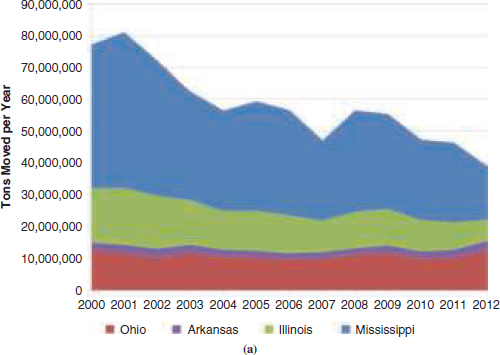
FIGURE 2-5 Annual trends by river in (a) midnation food and farm products.
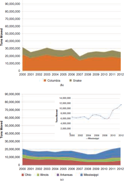
FIGURE 2-5 Annual trends by river in (b) northwestern food and farm products and (c) midnation petroleum and petroleum products (with inset showing a doubling of volumes on the Mississippi).
SOURCE: USACE Lock Use, Performance, and Characteristics, http://www.navigationdatacenter.us/lpms/lpms.htm, Locks by Waterway, Tons Locked by Commodity Group, Calendar Years 1993–2013. Accessed July 2014.
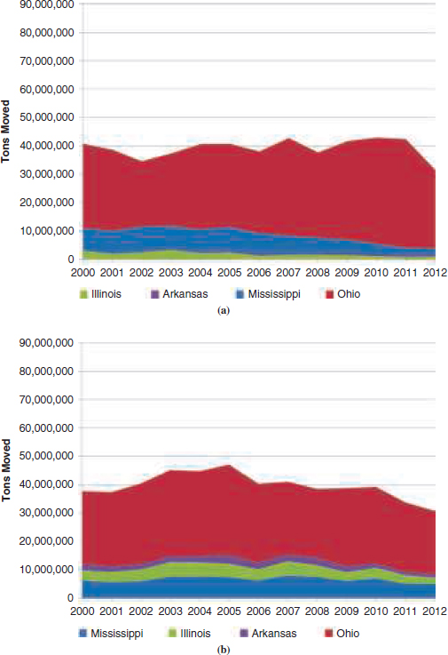
FIGURE 2-6 Annual trends by river in (a) midnation coal, lignite, and coal coke; (b) midnation crude materials.
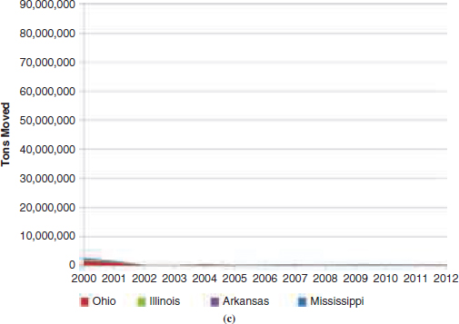
FIGURE 2-6 Annual trends by river in (c) midnation manufactured equipment and machinery.
SOURCE: USACE Lock Use, Performance, and Characteristics, http://www.navigationdatacenter.us/lpms/lpms.htm, Locks by Waterway, Tons Locked by Commodity Group, Calendar Years 1993–2013. Accessed July 2014.
text of potential mode shift is difficult because the modes are so different in their evolution, ownership, and funding. Furthermore, the ability of bulk cargoes to shift from one mode to another can depend on the availability of large-scale facilities to transfer cargo; thus, the potential for mode shift in the short run may vary from the potential in the long run.
Quantitative comparisons of freight movements across modes for a single cargo between a specific origin and destination are not considered here because they depend on such fluctuating factors as market conditions and the price of fuel and so are valid only for a short period of time. The more enduring observations on freight flows and mode shares can be useful in considering the impact of other modes on use of the inland waterways system.
Freight Flows
Examination of freight flows by mode shows the different character and magnitudes of cargoes moved. Figure 2-7 shows estimated U.S. freight flows by highway, rail, and waterway (http://www.ops.fhwa.dot.gov/freight/freight_analysis/nat_freight_stats/tonhwyrrww2010.htm). At an overview level the figure indicates that the modes are mainly complementary to one another instead of competing, although intense competition between rail and water occurs when facilities are being located and diminishes once a shipper or receiver has invested in facilities to support the preferred mode. One striking image is the heavy flow of coal by rail from the Powder River Basin to the Midwest, which complements the heavy waterway flows on the Mississippi and Ohio Rivers. Significant rail flows are notably absent parallel to the six waterway corridors studied, which may reflect the unwillingness or inability of railroads to compete in the short run for bulk cargoes that have ready access to water transportation. Truck traffic is heavy along the six waterway corridors, but trucks are a poor substitute for long-distance inland waterways transport because barges can carry more weight at a far lower cost than can trucks.
Modal Shares and Potential for Modal Shift
According to the U.S. Department of Transportation Freight Analysis Framework, Version 3 (FAF3),9 the relative modal shares of domestic tons and ton-miles of freight shipments remained similar across 1997, 2002, 2007, and 2012. As shown in Table 2-4, waterborne transport (which includes inland, lakewise, and coastwise movements) moves nearly 10 percent of all ton-miles in the national freight system. Comparable data are reported in Table 1-50 of the National Transportation
________________
9 The FAF category for “water” shown in Table 2-4 includes more than cargo moved on the inland waterways system—it also includes deep sea, coastal waters, and Great Lakes cargo movements. Furthermore, information included in the FAF differs from that available from the USACE Waterborne Commerce Statistics Center partly because of differences in statistical sourcing (such as in commodity classifications) and aggregation. However, the FAF is useful for an overview of the relative modal share values even though some of the absolute values that make up this general picture might differ from other sources.
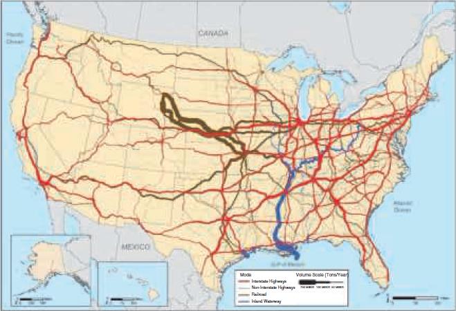
FIGURE 2-7 Freight flows by highway, railroad, and waterway, 2010, according to the Freight Analysis Framework, Version 3.
SOURCE: Freight Analysis Framework, Version 3, Freight Facts and Figures 2013 (http://www.ops.fhwa.dot.gov/freight/freight_analysis/nat_freight_stats/docs/13factsfigures/figure3_01.htm, accessed September 2014). (Highways, U.S. Department of Transportation, Federal Highway Administration, Freight Analysis Framework, Version 3.4, 2013; rail, based on Surface Transportation Board, Annual Carload Waybill Sample and rail freight flow assignments done by Oak Ridge National Laboratory; inland waterways, USACE, Institute of Water Resources, Annual Vessel Operating Activity and Lock Performance Monitoring System data, 2013.)
TABLE 2-4 Mode Share by Value, Freight Tons Moved, and Ton-Miles of Freight for 1997, 2002, 2007, and 2012 According to FAF3
| 1997 | 2002 | 2007 | 2012 | |
| Mode Share by Value | ||||
| Truck | 63 | 70 | 63 | 63 |
| Rail | 6 | 5 | 6 | 6 |
| Water | 0.7 | 0.7 | 1.2 | 1.3 |
| Air (including truck–air) | 10 | 4 | 4 | 5 |
| Multiple modes and mail | 16 | 15 | 20 | 19 |
| Pipeline | 2 | 2 | 4 | 4 |
| Other and unknown | 2 | 2 | 2 | 2 |
| Total | 100 | 100 | 100 | 100 |
| Mode Share by Freight Tons Moved | ||||
| Truck | 48 | 50 | 46 | 46 |
| Rail | 22 | 25 | 27 | 27 |
| Water | 7 | 7 | 6 | 6 |
| Air (including truck–air) | 0.1 | 0.1 | 0.1 | 0.1 |
| Multiple modes and mail | 5 | 5 | 7 | 7 |
| Pipeline | 16 | 12 | 12 | 13 |
| Other and unknown | 2 | 1 | 1 | 1 |
| Total | 100 | 100 | 100 | 100 |
| Mode Share by Ton-Miles of Freight | ||||
| Truck | 30 | 34 | 32 | 32 |
| Rail | 24 | 29 | 31 | 32 |
| Water | 9 | 8 | 9 | 10 |
| Air (including truck–air) | 0.3 | 0.1 | 0.2 | 0.2 |
| Multiple modes and mail | 11 | 10 | 10 | 10 |
| Pipeline | 23 | 17 | 17 | 15 |
| Other and unknown | 2 | 2 | 1 | 1 |
| Total | 100 | 100 | 100 | 100 |
NOTE: Mode shares are expressed as percentages.
Statistics, 2013, where the ton-miles accounted for by multiple-mode shipments are redistributed to the individual modes.
Choice of mode and intermodal combinations is affected by such factors as access to an alternative mode (DiPietro et al. 2014), time to delivery, cost, transparency of tracking, flexibility if rerouting may be required (Simmons et al. 2013), and payload per shipment (Kruse et al. 2012). Inland waterborne commerce requires more time to delivery than other modes for similar transport distances because (a) shallow water navigation speeds with heavy payloads are slower than road or rail speeds and (b) routes can be longer because waterways are circuitous. Longer distances and transit times do not necessarily preclude use of a modal shift to barge, particularly as energy prices, freight rates, and other drivers favoring larger payloads on intermodal networks may emerge. Judgments about modal trade-offs, including those related to concerns about shifts from barge as described in Box 2-1, need to be informed by transparent and rigorous analyses beyond the scope of this report.
Condition and Performance of Inland Waterways Infrastructure
OVERVIEW
The availability of multiple measures of system reliability and performance is useful for assessing system functioning. Delays, lock unavailabilities, and usage of the system are important components in the assessment of system functioning and are the focus of this section. USACE maintains multiple measures of performance as part of a Lock Performance Monitoring System (http://www.navigationdatacenter.us/lpms/lpms.htm) used here to describe the performance of lock infrastructure. Lock performance metrics derived from these measures could be useful in a systemwide assessment of locks for asset management and setting of maintenance priorities (see Chapter 4).10 Data enhancements
________________
10 The USACE Lock Performance Monitoring System contains 10 measures of cargo transported through the locks, nine commodity groups and one total tons metric. Sixteen metrics describe facility use intensity and performance for commercial, noncommercial, and recreational navigation. They include hours of processing and delay time; vessel, barge, and tow counts; and numbers of lockages. Six metrics describe lock closure statistics, including unscheduled and scheduled unavailabilities in terms of both number (frequency) and annual hours closed.
BOX 2-1
Modal Shift to Road or Rail Resulting from Loss of Waterway Corridor
The Transportation Research Board’s Executive Committee wanted this study to cover possible impacts of a major diversion of freight from water on highway systems should a waterway fail because of deferred maintenance. In view of the volume that can be moved by one barge being equal to the payloads of many trucks, state officials have expressed concern about the consequences of massive numbers of heavy trucks replacing shipments that had moved by water for highway congestion and pavement and bridge infrastructure.
Long-duration (more than 6 months) closures of waterways have been rare. Few year-long navigation closures of major lock and dam installations have occurred in the past 20 years, and only four locks on high-use waterways have been out of service for more than 180 days in any year since 1993.a USACE uses scheduled closures, intermittent closures during phased construction, and other design and construction strategies to minimize the impact of long-duration construction and repair, similar to current practices for highway repair and construction that balance long-duration full closures with partial closures or intermittent closure periods.
When a section of infrastructure is out of service for months or longer, shippers have multiple choices, including rerouting, postponing, or canceling shipments; selling goods in different markets; and, if the loss is sufficiently disruptive and alternative modes too costly, closing (DiPietro et al. 2014). For barge transportation, the simplifying assumption is usually made that in the event of a waterway closure, most freight that could shift would shift to rail and relatively little to truck, because of the substantially greater cost of movement by truck (Kruse et al. 2011). Modeling and analysis of what might happen to soybean shipments if various locks closed on the Upper Mississippi, Illinois, or Ohio Rivers indicated that total shipments of soybeans would decrease, but the rail mode share would increase and the truck share decrease (Kruse et al. 2011). However, the outcomes in specific corridors depend on circumstances, and some modal shift to truck cannot be ruled out. Furthermore, substantial drayage transport may be needed in a water-to-rail shift (i.e., short-distance
________________
a These statistics are derived from the committee’s analysis of USACE unavailability data collected for the USACE Lock Performance Monitoring System, http://www.navigationdatacenter.us/lpms/data/lock2013webunavail-021914.htm.
trucking to connect the origin with rail via partial waterway movement or to connect the origin directly with rail access).
Impacts from such an event would vary widely by corridor, commodity, and the nature of freight flows in the corridor. Because a loss of transportation access can shift markets and shipper behavior in complex ways, accurate predictions concerning modal shifts cannot be made without a detailed analysis and model applied to a suite of case studies.
that could improve understanding of traffic flows and be used to set priorities to maintain reliable freight service are noted as part of this discussion and are elaborated on further in Chapter 4. Options for metrics are discussed in Appendix E of this report and in Chapter 4.
USACE also maintains statistics on the original construction of locks (construction year, gate type, safety, and so on), which are publicly available (http://www.navigationdatacenter.us/index.htm). The statistics describe the design details of lock and dam infrastructure and so could be useful in determining the condition of locks as part of a systemwide assessment. Other important information for assessing condition, such as records on major rehabilitations and seasonal navigation closures, is not available for all lock and dam facilities in an identifiable location that is accessible to the public but would be desirable for system assessment.
Lock age does not measure performance and is not included in the USACE Lock Performance Monitoring System. It is included in this discussion because the age of locks is widely used to communicate the condition of the inland waterways system and needs for funding.
AGE OF LOCKS
Figure 2-8 shows a map of inland waterways lock infrastructure by original construction date. Figure 2-9 shows the average age of lock and dam infrastructure in comparison with other federal and state infrastructure and transportation assets. The average age of the locks in 1940 was less than 10 years; in 1980 the average age of the locks was about 30 years (whether or not major rehabilitation work was considered); in 2014 the average age was 59 years.
FIGURE 2-8 Summary map of inland waterways navigation lock and dam infrastructure, by year of construction.
SOURCE: USACE Navigation Data Center GIS Viewer files (http://www.navigationdatacenter.us/db/gisviewer/) and Lock Use, Performance, and Characteristics (http://www.navigationdatacenter.us/lpms/lpms.htm). Accessed July 2014.
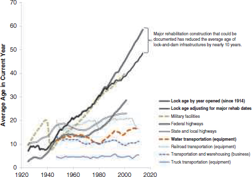
FIGURE 2-9 Comparison of age of infrastructure showing inland navigation lock age (with and without consideration of rehabilitation construction).
SOURCE: USACE Navigation Data Center: Lock Use, Performance, and Characteristics, http://www.navigationdatacenter.us/data/datalck.htm, accessed July 2014.
A substantial number of locks have been rehabilitated, which would be expected to restore performance to its original condition if not better and effectively reduce the age of the locks. To illustrate the impact, for this report, the effective age of locks was updated (assumed to return to zero) for locks on the Illinois, Mississippi, and Ohio River system where major rehabilitation was documented. This approach is similar to that used for documenting the current age of highways, bridges, and military infrastructure and is a more accurate method of communicating the age of inland waterways infrastructure.
In 2014, the average age of locks computed from the date of last known major rehabilitation was 49 years, nearly 10 years younger than the age assessed from the original construction date (Figure 2-9;
see Appendix C for documented dates of original construction and last known major rehabilitation; see Appendix D for age detail for each major river system.)11 After rehabilitation is accounted for, in 2014 more than 50 percent of the locks were more than 50 years old (Figure 2-10a). However, rehabilitated age varies substantially by river system. For example, the Ohio River corridor is about 6 years (10 percent) younger than the original construction age when age is adjusted for major rehabilitation construction (Figure 2-10b), while locks on the Upper Mississippi and Illinois River (Figure 2-10c) have an age adjusted from construction of about 36 years, less than half of the age reckoned from original construction.
USAGE
Usage of navigation locks can be computed in several ways, such as by transported commerce (tonnage) or by number of cycles (lockages). Consideration of lock tonnage (Figure 2-11) and the number of lockages (Figure 2-12) together is useful because it provides insight into the importance of locks in the waterway. The highest-use locks by lock tonnage are found along high- and moderate-use waterways, primarily the Upper Mississippi and Ohio River corridors (Figure 2-11).12 High-use cargo locks frequently have a large number of lockages, which is understandable given the large number of barges that travel through them. An exception is small locks that require multiple lockages for typical barge tows. The eight river systems with the most average lockages per lock are shown in Figure 2-13: the Ohio (including Monongahela and Allegheny), the GIWW, the Upper Mississippi, the Arkansas, the Illinois, the Tennessee, the Tennessee–Tombigbee, and the Columbia (including the Snake) systems. They account for more than 77 percent of all lockages in the inland waterways.
Some locks that experience periods of high use are on waterways designated as low or moderate use on the basis of average annual ton-miles, which has implications for the allocation of resources needed
________________
11 See Chapter 4 for further discussion of age of infrastructure in the context of asset management and prioritization of maintenance spending.
12 As described earlier, high-use waterways are defined by USACE as those carrying more than 3 billion ton-miles of freight annually. Medium-use waterways carry 1 billion to 3 billion ton-miles of freight annually, and low-use waterways carry less than 1 billion ton-miles annually.
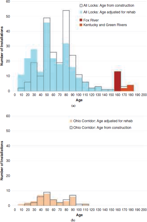
FIGURE 2-10 Histogram of effective age of infrastructure on the inland waterways network including rehabilitation for (a) all locks using available data, (b) the Ohio River corridor.
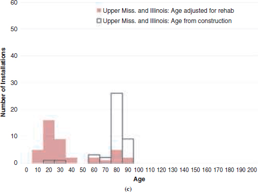
FIGURE 2-10 Histogram of effective age of infrastructure on the inland waterways network including rehabilitation for (c) the Upper Mississippi and Illinois River corridors.
SOURCE: USACE Navigation Data Center: Lock Use, Performance, and Characteristics, http://www.navigationdatacenter.us/data/datalck.htm, accessed July 2014.
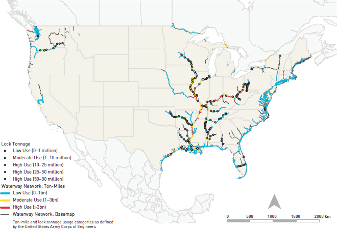
FIGURE 2-11 Summary of number of tons of cargo passing through inland waterway navigation lock and dam infrastructure, with waterways identified according to ton-mile usage category and locks identified by ton usage category.
SOURCE: USACE Navigation Data Center, GIS Viewer files, http://www.navigationdatacenter.us/db/gisviewer/; Lock Use, Performance, and Characteristics, http://www.navigationdatacenter.us/lpms/lpms.htm. Accessed July 2014. Usage definitions based on USACE 2013, Table F-1 and Section F-12.
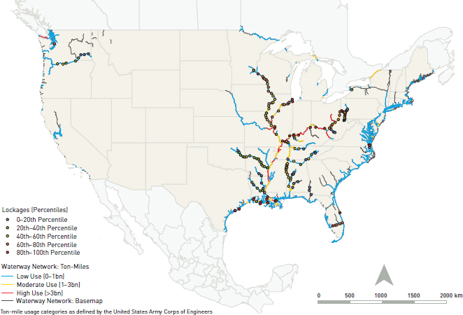
FIGURE 2-12 Summary of inland waterways navigation lock and dam usage, by percentage of lockages in the inland navigation system (2013 data).
SOURCE: USACE Navigation Data Center, GIS Viewer files, http://www.navigationdatacenter.us/db/gisviewer/; Lock Use, Performance, and Characteristics, http://www.navigationdatacenter.us/lpms/lpms.htm. Accessed July 2014.
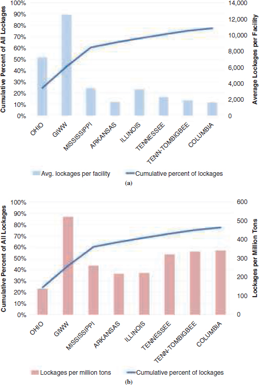
FIGURE 2-13 Summary of top eight rivers by lockages and cumulative percent of lockages by (a) lockages per facility on the river and (b) lockages per million tons transported. These eight rivers account for about 80 percent of all lockages in the inland waterways system.
SOURCE: USACE Lock Use, Performance, and Characteristics, http://www.navigationdatacenter.us/lpms/lpms.htm, Locks by Waterway, Lock Usage, Calendar Years 1993–2013. Accessed July 2014.
to maintain the system. For example, whereas the entire Arkansas and Tennessee Rivers are low use, the Upper Mississippi, Illinois, and Tennessee–Tombigbee Rivers and the GIWW have high-use locks in waterway sections that would be classified as moderate or low use. This situation can occur because of seasonal peaks in the movement of certain commodities such as harvested food and farm products or because of navigation closures due to annually recurring weather conditions such as ice or flooding. For prioritization, the tonnage moved through each lock during peak demand periods, as well as the type and value of the cargo, needs to be considered; usage should not be assessed merely on the basis of average annual waterway ton-miles. Likewise, some rivers and waterborne corridors may on a seasonal basis move as much or more tonnage as rivers classified as high use but receive low-use classification on the basis of annual ton-miles of transport rather than seasonal peak ton-miles.
River systems have sharply different patterns with regard to the direction and balance of freight flows, which has implications for the economic importance of low-use tributaries to the system. These patterns are shown in Figure 2-11 for tonnage and in Figure 2-12 for lockages. To illustrate, the Ohio system, which mainly carries coal, is self-contained, with balanced flows back and forth; low-use tributaries make little contribution to overall system flows. However, the Upper Mississippi and Missouri Rivers are part of an export-based system in which low-use tributaries contribute to increases in the tonnages of food and farm products and other types of freight carried as barges move downstream.
Some busy locks on low-use waterways near major population centers do not move freight but provide service for recreational navigation. For example, the Okeechobee Waterway and the Albemarle and Chesapeake Canal have low-tonnage locks that experience a large number of recreational lockages. Such facilities might be candidates for charging recreational users for lockage.
DELAYS AND UNAVAILABILITIES
The definitions and measures used in this section are consistent with terminology and performance measures included in the USACE Lock Performance Monitoring System (http://www.navigationdatacenter
.us/lpms/lpms.htm). Lost transportation time is the average time lost by vessel tows to unproductive transportation. It is the sum of delay and unavailability. Lost transportation time due to delays and lock unavailability is a cost to shippers and an important consideration in deciding on future investments to maintain reliable freight service. A delay is defined by USACE as the time a tow must wait to move through a lock once it is at the lock and ready to transit (i.e., to be processed through the lock). Lock unavailability is a closure or outage usually due to failure or repair.
Some delays and unavailabilities are expected in any transportation network. As cargo moves up- and downriver, delays can occur if the barge tow is too large and must be towed through in sections; if there is a backlog of barges waiting to be towed through the lock; or if the lock experiences an outage for routine maintenance, weather, accident, equipment failure, or other unforeseen reasons. Operators may be waiting for shippers to bring cargo to the waterfront; cargoes must be safely loaded into vessels and barges; lockages require processing time to prepare chambers and gates, which can result in delays for other vessels; and queuing (congestion) may occur during peak usage times.
The number and duration of some delays and unavailabilities may indicate declining performance of navigation locks because of aging machinery or infrastructure (unreliability) or a mismatch between lock sizes and demand for vessels and cargoes (undercapacity). Delays also can occur on river segments without lock and dam infrastructure because of flood conditions or low-water periods; a summary of waterway locations where noninfrastructure delays may occur is not included in USACE performance statistics.13
USACE maintains public statistics on annual delays for each lock and dam, scheduled unavailabilities, and unscheduled unavailabilities.14Delay is reported by using average time delayed per delayed vessel and the percentage of vessels delayed. Annual delay is estimated
________________
13 USACE could address this gap in performance data by providing information in future data releases on delays for river segments without lock and dam infrastructure beyond the data already available on delays due to dredging.
14 Unavailability statistics are at http://www.navigationdatacenter.us/lpms/data/lock2013webunavail021914.htm; commodity statistics are at http://www.navigationdatacenter.us/lpms/cy2013comweb.htm; usage statistics are at http://www.navigationdatacenter.us/lpms/lock2013web.htm.
by multiplying the total vessels transiting a lock by average delay time per vessel. These statistics can be organized by river or aggregated to represent the potential lost service in hours for the waterways system as a whole. Lock processing time is not included in the USACE definition and measure of delay and is instead a separate measure in the USACE Lock Performance Monitoring System. Lock processing time is the time required for a vessel to approach, to break down the tow into subtows (if needed for large tows to pass through the lock), to enter the lock chamber, for the water level to rise or fall, for the vessel to exist and clear the lock, and to reassemble the tow (if needed).15 The description of the system that follows maintains this distinction and examines lock processing time separately from delay because (a) such a procedure is consistent with USACE’s performance metrics, (b) the underlying causes and mitigation of these occurrences may differ, and (c) stakeholders informed the committee during public meetings that outages (unscheduled unavailabilities) are a primary concern for the reliability of shipping service.
Figure 2-14 shows the percentage of vessels delayed on low-, moderate-, and high-use segments of the system. On average, 49 percent of tows in 2013 were delayed across the 10 highest-tonnage locks, with an average length of tow delay of 3.8 hours. USACE’s Lock Performance Monitoring System does not include the reasons for delay.16 Delays might be attributable to seasonal peak volumes due to weather, harvest, undercapacity, or other causes. However, the observation that delays are typically larger at locks with greater demand for agriculture-related transport during the harvest period suggests that the delays are largely a result of seasonal congestion.
Unavailabilities are reported by using the number of outages and the total hours unavailable per year.17 For 2000 through 2013 the
________________
15 USACE’s measure of lock processing time does not distinguish processing times specific to the locking through of tows larger than the lock. However, the extra waiting time imposed on other tows because of lockage reconfiguration activities is captured in the lock delay time.
16 Collecting information about the reasons for delay would be useful for prioritization, as discussed in Chapter 4.
17 The time that the lock is unavailable due to scheduled or unscheduled maintenance is not considered delay in the USACE Lock Performance Monitoring System statistics but is tracked separately. (Delay presumes that the lock is open, whereas if a lock is unavailable it is scheduled as closed or experiencing an unanticipated outage.) Figure 2-16b illustrates the importance of the distinction.
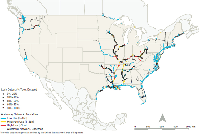
FIGURE 2-14 Summary of inland waterways navigation lock and dam delay statistics, by percent of vessels delayed (2013 data).
SOURCE: USACE Navigation Data Center, GIS Viewer files, http://www.navigationdatacenter.us/db/gisviewer/; Lock Use, Performance, and Characteristics, http://www.navigationdatacenter.us/lpms/lpms.htm. Accessed July 2014.
estimated lost transportation hours due to delays accounted for nearly 80 percent of the total hours in lost service (Figure 2-15). More hours of lost transportation time are attributable to scheduled unavailability than to unscheduled outages. As discussed below, a method is needed for understanding the impact of delay and unavailabilities across the system to determine proper approaches for mitigating delay.
MODEL FOR UNDERSTANDING THE POTENTIAL IMPACT OF DELAY AND UNAVAILABILITY
To improve understanding of the impact that delay and unavailability can have on service, the transportation hours lost because of scheduled
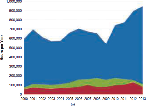
FIGURE 2-15 Summary of trends in total lost transportation time (delays and unavailabilities): (a) in hours per year for all locks and dams.
SOURCE: USACE Lock Use, Performance, and Characteristics, http://www.navigationdatacenter.us/lpms/lpms.htm, Locks by Waterway, Lock Usage, Calendar Years 1993–2013, and Locks by Waterway, Locks Unavailability, Calendar Years 1993–2013. Accessed July 2014.
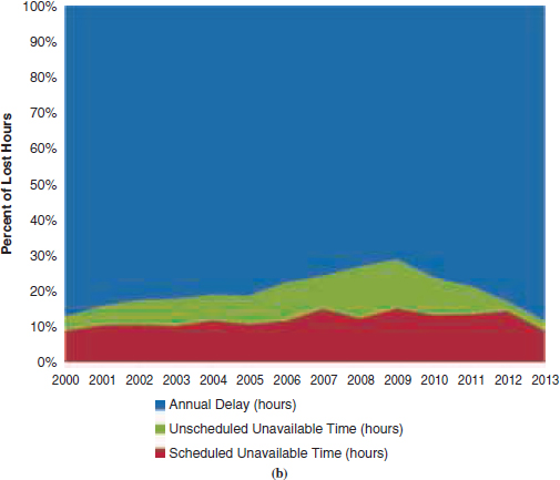
FIGURE 2-15 Summary of trends in total lost transportation time (delays and unavailabilities): (b) as percents of lost hours for all locks and dams.
and unscheduled delay can be evaluated for specific locks and dams and considered in the light of navigation demand. Demand can be observed in terms of (a) tonnage of cargo transported, (b) number of vessels requiring passage through locks, and (c) the number of lockages (i.e., use of navigation infrastructure). Lock infrastructure for a river system can be compared with regard to long-run demand (cargo transported, vessels, and lockages) and chronic lost service (hours of delay and hours unavailable). By averaging these data over a number of years, periodic influences such as short-term economic downturns can be minimized. (See Appendix E for an illustration for several sets of locks and dams grouped by major river system.) A derived metric,
such as average lost transportation hours per million tons of cargo, could be a useful way of identifying and prioritizing facilities for investment consideration.18
To illustrate, Figure 2-16a shows the average percentage of lock transit time accounted for by lock processing time versus lost transportation hours, which comprises delay and unavailability. Systemwide, the inland waterways had an annual average of 272 lost transportation hours per million tons of commerce from 2000 through 2013, according to data obtained from USACE. A detailed examination of lost transportation hours shows that lost transportation time was dominated by delay, as illustrated in Figure 2-16b. Each river and corridor may have its unique characteristic metric, which would be a function of the commodities served, seasonality, and performance of the lock and dam infrastructure. Identifying major facilities where the lost transportation time due to delay or repairs is significantly higher than the river average could improve investment decisions to preserve or upgrade navigation performance.
Several options exist for mitigating hours of lost transportation service. Among them are the following:
- An effective system for scheduling lock usage to reduce queuing congestion (discussed further in Chapter 3); this may require users to invest in increased storage for waterborne commodities during peak demand periods such as the harvest;
- Localized reprioritization of lock throughput design that could consider seasonal peak demand (often driven by late spring ice melts, summer flooding, or early winter freezes); this may involve realigning the USACE construction investment framework away from annualized benefits in regions where infrastructure is critical to peak seasonal usage (e.g., Illinois River food and farm products); and
- Continued attention to managing unavailabilities and pursuit of opportunities for avoiding such closures (scheduled or unscheduled); investment in more operations and maintenance (O&M)
________________
18 The average accounts for the elements of delay that occur as more tonnage is moved through the waterway network.
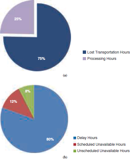
FIGURE 2-16 (a) Summary of lock transit time: processing hours versus lost transportation hours and (b) detailed breakdown of lost transportation hours as delay and scheduled or unscheduled unavailability. Lost transportation hours are reported in terms of hours per million tons of commerce for 2000–2013.
SOURCE: USACE Lock Use, Performance, and Characteristics, http://www.navigationdatacenter.us/lpms/lpms.htm, Locks by Waterway, Lock Usage, Calendar Years 1993–2013, and Locks by Waterway, Locks Unavailability, Calendar Years 1993–2013. Accessed July 2014.
activities to reduce lost transportation time due to outages may be economically more beneficial than capital investments to expand the size of locks.
Data are not available to explain the causes of delay at locks, which makes up 80 percent of lost transportation hours. Delay might be attributable to seasonal peak volumes due to weather, harvest, undercapacity, or other causes. Collection of data and development of performance metrics would enhance understanding of whether delay problems could be most efficiently addressed by more targeted O&M, traffic management, capacity enhancement, or some combination of these measures (see Chapter 4). Such an index would be superior to the proxy of age, which is an inconsistent indicator of lock infrastructure failure. As shown in Table 2-5, measures of lock performance are for the most part not correlated with age of locks.
The role of the inland waterways system in freight transportation has changed significantly since the system was built to promote the early economic development of the nation. Today, barges carry a relatively small but steady portion of freight, mainly bulk commodities that include coal, petroleum and petroleum products, food and farm products, chemicals and related products, crude materials, manufactured goods, and manufactured equipment. Annual trends in inland waterways shipments show that freight traffic is static or declining on some waterways. Overall demand for the inland waterways system is static relative to the growing demand for rail and truck. In recent years, the inland waterways system has transported 6 to 7 percent of all domestic cargo (measured in ton-miles). Truck has carried the greatest share of freight, followed by rail, pipeline, and water.
Seventy-six percent of barge cargo (in ton-miles) moves on just 22 percent of the 36,000 inland waterway miles. About 50 percent of the inland waterway ton-miles moves on six major corridors
TABLE 2-5 Summary of Correlations Between Lock Performance and Lock Age in 2014 Calculated from the Date of Last Known Major Rehabilitation
| River System | Average Age of Locks | Level of Correlation Between Lock Performance and Effective Age on a River System | ||||||
| Lockages | Percent of Vessels Delayed | Percent of Tows Delayed | Average Vessel Delay | Average Tow Delay | Average Closure Duration | Closure Frequency | ||
| All inland river locks | 61 | Low | Low | Low | Low | Low | Low | Low |
| Ohio River | 35 | Low | Low | Low | Low | Low | Low | Low |
| Mississippi River | 25 | Low | Low | Low | Low | Low | Medium | Low |
| Illinois River | 22 | Medium | Low | Low | Low | Low | Medium | Medium |
| Columbia–Snake Rivers | 45 | Low | Low | Low | Low | Low | High | Low |
| GIWW | 72 | Low | Low | Low | Low | Low | Low | Low |
| Arkansas River | 45 | Low | Medium | Medium | Medium | Low | Low | Low |
| River System | Average Age of Locks | Level of Correlation Between Lock Performance and Effective Age on a River System | ||||||
| Lockages | Percent of Vessels Delayed | Percent of Tows Delayed | Average Vessel Delay | Average Tow Delay | Average Closure Duration | Closure Frequency | ||
| Black Warrior, Tennessee, Tennessee–Tombigbee, Tombigbee | 42 | Low | Medium | Medium | Low | Low | Low | Medium |
| Monongahela River | 57 | Medium | High | High | Medium | Low | Gaps in data | Medium |
| Allegheny River | 62 | Low | Low | Low | Low | Low | Gaps in data | Low |
NOTE: Delay and closure (includes scheduled and unscheduled unavailability) data used to compute correlations were obtained from the USACE Lock Performance Monitoring System. High positive correlation (blue text, blue shading) is defined as greater than 75 percent correlation. Medium positive correlation (blue text, light blue shading) is defined as between 50 and 75 percent correlation. Medium negative correlation (red text, light pink shading) is defined as between -50 and -75 percent correlation. Low correlation (white background) is defined as within ±50 percent correlation. Some rivers indicate “negative correlations” because the correlations are affected by traffic level and rehabilitation; that is, some of the older locks have less traffic and so fewer traffic-related problems, or they may be rehabilitated and so experience fewer closures and delays. (See Appendix F data detail.)
SOURCE: USACE Lock Use, Performance, and Characteristics, http://www.navigationdatacenter.us/lpms/lpms.htm: Locks by Waterway, Tons Locked by Commodity Group, Calendar Years 1993–2013; Locks by Waterway, Lock Usage, Calendar Years 1993–2013; and Locks by Waterway, Locks Unavailability, Calendar Years 1993–2013. Accessed July 2014.
that represent 16 percent of the inland waterway miles—the Upper Mississippi River, the Illinois River, the Ohio River, the Lower Mississippi River, the Columbia River system, and the GIWW. Some inland waterways segments have minimal or no freight traffic. With shrinking resources for the system and growing demands on the USACE O&M budget, targeting commercial navigation investments mainly to portions of the system important for moving freight would be prudent.
Lost transportation time due to delays and lock unavailability (outages) is a cost to shippers and an important consideration in deciding on future investments. Systemwide, about 80 percent of lost transportation time is attributable to delays. On average, 49 percent of tows in 2013 were delayed across the 10 highest-tonnage locks, with an average length of tow delay of 3.8 hours. Some delay is expected for routine maintenance, weather, accidents, and other reasons, but delays can be affected by maintenance outages caused by decreases in the reliability of aging machinery or infrastructure. About 12 percent of lost time on the inland waterways system is due to scheduled closures and about 8 percent is due to unscheduled closures, which indicates that up to 20 percent of lost time could be addressed with more targeted O&M resources. Targeting O&M resources toward major facilities with frequent lockages and high volumes and where the lost time due to delay is significantly higher than the river average could improve navigation performance.
Most lost service due to delay occurs at high-demand locks used for agricultural exports and so may be caused by congestion related to peaks in seasonal shipping. Chapter 4 describes debates about how to mitigate congestion delays. Data are not available to explain the causes of delay at locks, which makes up 80 percent of lost transportation hours. Delays might be attributable to seasonal peak volumes due to weather, harvest, undercapacity, or other causes. Collection of data and development of performance metrics would enhance understanding of whether delay problems could be most efficiently addressed by more targeted O&M, traffic
management, capacity enhancement, or some combination of these measures.
Some high-use locks are located on waterways designated as low or moderate use, which has implications for how to allocate funds across parts of the system. This situation can occur because of seasonal peaks in the movement of certain commodities, such as harvested food and farm products, or from navigation closures caused by annually recurring weather conditions, such as ice or flooding. The tonnage moved through each lock during peak demand periods, as well as the type and value of the cargo, could be considered in funding allocations instead of considering only average annual waterway ton-miles. Likewise, some rivers and waterborne corridors may move as much or more tonnage on a seasonal basis as rivers classified as high use but receive low-use classification on the basis of annual ton-miles of transport rather than seasonal peak ton-miles.19
The advanced age of lock and dam infrastructure is often used to communicate funding needs for the system. Age is not a good indicator of lock condition. A substantial number of locks have been rehabilitated, which would be expected to restore performance to its original condition if not better. Dating the age of assets from the time of the last major rehabilitation, as is done for highway infrastructure such as bridges, would be more accurate. Furthermore, with some exceptions, little correlation exists between the age of locks and their performance as measured by delay experienced by system users. A more useful approach for targeting funds to improve system performance than focusing on age as a proxy for lock functioning would be to identify waterway segments and facilities where the lost time due to delay (based on millions of tons delayed) is substantially higher than the system average.
________________
19 An approach to prioritization focusing on economic risk, such as that discussed in Chapter 4, would address whether an outage during a seasonal peak could be more costly than an outage occurring on a segment with fairly level year-round traffic.
References
ABBREVIATIONS
| AASHTO | American Association of State Highway and Transportation Officials |
| CMTS | Committee on the Marine Transportation System |
| TRB | Transportation Research Board |
| USACE | U.S. Army Corps of Engineers |
AASHTO. 2013. Waterborne Freight Transportation: Bottom Line Report. Washington, D.C. http://www.camsys.com/pubs/WFT-1_sm.pdf.
Clark, C., K. E. Hendrickson, and P. Thoma. 2012. An Overview of the U.S. Inland Waterway System. IWR Report 05-NETS-R-12. Institute of Water Resources, U.S. Army Corps of Engineers, Alexandria, Va.
CMTS. 2008. National Strategy for the Marine Transportation System: A Framework for Action. U.S. Department of Transportation, Washington, D.C. http://www.cmts.gov/downloads/National_Strategy_MTS_2008.pdf.
DiPietro, G. S., H. S. Matthews, and C. T. Hendrickson. 2014. Estimating Economic and Resilience Consequences of Potential Navigation Infrastructure Failures: A Case Study of the Monongahela River. Transportation Research Part A: Policy and Practice, Vol. 69, pp. 142–164.
Kruse, C. J., A. Protopapas, Z. Ahmedov, B. McCarl, X. Wu, and J. Mjelde. 2011. America’s Locks and Dams: A Ticking Time Bomb for Agriculture. Texas A&M Transportation Institute and Department of Agricultural Economics, Texas A&M University, College Station.
Kruse, C. J., A. Protopapas, and L. E. Olsen. 2012. A Modal Comparison of Freight Transportation Effects on the General Public (2001–2009). Prepared for the National Waterways Foundation by Texas Transportation Institute, Texas A&M University, College Station.
Kruse, C. J., A. Protopapas, L. E. Olsen, and D. Bierling. 2007. A Modal Comparison of Freight Transportation Effects on the General Public. Texas Transportation Institute, Texas A&M University, College Station.
McCartney, B. L., L. L. Ebner, L. Z. Hales, and E. Nelson. 1998. Inland Navigation: Locks, Dams, and Channels. ASCE Manuals and Reports on Engineering Practice No. 94. American Society of Civil Engineers, Reston, Va.
National Park Service. 2013. Transportation: Trails and Roads, Canals and Railroads. http://www.nps.gov/nr/travel/ohioeriecanal/transportation.htm. Accessed May 14, 2014.
Simmons, S., K. Casavant, and J. Sage. 2013. Real-Time Assessment of the Columbia–Snake River Extended Lock Outage: Process and Impacts. In Transportation
Research Record: Journal of the Transportation Research Board, No. 2330, Transportation Research Board of the National Academies, Washington, D.C., pp. 95–102.
TRB. 2004. Special Report 279: The Marine Transportation System and the Federal Role: Measuring Performance, Targeting Improvement. Transportation Research Board of the National Academies, Washington, D.C. http://onlinepubs.trb.org/onlinepubs/sr/sr279.pdf.
USACE. 2013. Corps of Engineers Civil Works Direct Program, Budget Development Guidance, Fiscal Year 2015. Circular No. 11-2-204. Washington, D.C., March 31. http://www.cmanc.com/web/fy15ec_final.pdf.


