
Appendix B
Historical Development of ERS Rural-Urban Classification Systems
ABSTRACT
Since the 1970s, the Economic Research Service (ERS) of the U.S. Department of Agriculture (USDA) has taken the lead in developing and maintaining multilevel, rural-urban classification systems. ERS currently maintains four such systems that are widely used in social science research, policy development, and program administration. This paper traces the development of the Rural-Urban Continuum Codes, the Urban Influence Codes, the Rural-Urban Commuting Area Codes, and the Frontier and Remote Area Codes. Similarities and differences in underlying concepts, methodologies, criteria, data, and geographical building blocks are highlighted. Several factors drove the evolution of these systems: changing spatial concepts; changing federal policy needs; modifications to underlying Census/Office of Management and Budget (OMB) definitions; the desire to take advantage of new data and advancing GIS capabilities; and the need to keep pace with rapidly evolving rural-urban space. This historical evaluation will aid in ongoing efforts to help ensure the future validity of these classification systems as research and policy tools and to improve their usefulness for ERS and the broader research community.
INTRODUCTION
The Economic Research Service (ERS), USDA currently maintains four geographic classification systems that divide U.S. territory along rural and
urban dimensions (see Table B-1). All four are tied to metropolitan (metro) area concepts from the Office of Management and Budget (OMB) and build directly on the U.S. Census Bureau’s urban area definitions, especially the 50,000 population threshold as the basic “rural-urban” dividing line.1 All four move beyond the metro-nonmetro dichotomy, using Census urban geography and other criteria to devise multiple levels of rurality below the 50,000 population threshold. Two are county-based classifications that directly maintain the metro-nonmetro distinction among counties but add additional categories using measures of proximity and urban size. Two are based on smaller geographic units and different criteria but are anchored to the metro area concept by use of Census urbanized areas as their starting points.
In this paper, each classification system is described in the order it was developed, highlighting the changing historical context and the reasoning behind key decisions in the selection of criteria and methodology. The four classification systems were published at different times over 37 years (1975 to 2012) using different data sources and new ways of measuring key concepts such as population size, population density, and urban proximity or remoteness. These differences reflect prevailing spatial concepts at the time each classification was developed and the desire to keep pace with new patterns of population distribution during these decades. Modifications to underlying OMB and Census Bureau definitions, such as the introduction of micropolitan areas in 2000, contributed to the development of new classification criteria, as did the availability of new data and advances in computer processing capabilities.
The two county-based systems were originally developed solely to facilitate policy-relevant research at ERS and elsewhere, but have since been adapted for policy and program uses in various federal agencies. The two subcounty classifications were developed in partnership with the Office of Rural Health Policy, Department of Health and Human Services, to meet both research and programmatic requirements. All four were designed to help answer basic research questions important to USDA policy making: What are the economic needs and opportunities in different rural areas? What factors underlie those conditions and how have they shifted over time in response to economic shocks, industrial restructuring, and demographic change?
ERS has undertaken an in-depth assessment of these rural-urban classification systems, beginning with insights derived from this workshop.
_______________________
1The ERS topic page “What Is Rural?” describes how metro and nonmetro areas are defined and how they compare to Census urban and rural areas. See http://www.ers.usda.gov/topics/rural-economy-population/rural-classifications/what-is-rural.aspx [November 2015].
TABLE B-1 Economic Research Service (USDA) Rural-Urban Classification Codes
| Name | Geography | Categories | Criteria | Initial Release |
| Rural-Urban Continuum Codes (RUCC) | Counties | 9 categories: 3 metro 6 nonmetro | For metro counties: Population of metro area For nonmetro counties: Total urban population and adjacency to metro areas | 1975 |
| Urban Influence Codes (UIC) | Counties | 12 categories: 2 metro 10 nonmetro | For metro counties: Population of metro area For nonmetro counties: Size of largest city, adjacency to metro areas by size of metro area, and micropolitan status | 1997 |
| Rural-Urban Commuting Area (RUCA) Codes | Census tracts; results used to create a version based on zip code areas | 10 primary codes: 3 metro 7 nonmetro 30 secondary codes | Primary codes: Urban area size; size and direction of largest commuting flow Secondary codes: Size and direction of 2nd largest commuting flow | 1998 |
| Frontier and Remote (FAR) Codes | 1/2 x 1/2 kilometer grid cells; results aggregated to zip code areas | 4 (nested) levels | Travel times by car to edges of nearest urban areas by size, based on posted speed limits | 2012 |
SOURCE: Prepared by John Cromartie for his presentation. Based on USDA Economic Research Service. Available: http://www.ers.usda.gov/topics/rural-economy-population/rural-classifications.aspx [October 2015].
The purpose of the assessment is to help ensure the future validity of these classification systems as research and policy tools and to improve their usefulness for ERS and the broader research community. The following descriptions of the current classification systems and their historical development will help identify what considerations need to go into modifying existing rural-urban classifications and developing new ones (see http://www.ers.usda.gov/topics/rural-economy-population/ruralclassifications.aspx [November 2015]).
COUNTY-BASED DEFINITIONS
ERS researchers and others who analyze conditions in “rural” America most often study conditions in nonmetropolitan (nonmetro) areas, defined on the basis of counties. Counties are the basic building block for economic data and thus for conducting research to track and explain regional population and economic trends. Estimates of population, employment, and income are available at the county level annually. They also are frequently used as basic building blocks for areas of economic and social integration other than OMB metro areas, such as ERS labor-market areas and commuting zones.
Nonmetro counties are counties not part of larger metropolitan areas—that is, they do not contain urbanized areas of 50,000 or more residents or have 25 percent or more of their workforce commuting to counties containing urbanized area of this size. Nonmetropolitan counties include some combination of
- open countryside,
- rural towns (clusters of dense population with fewer than 2,500 people), and
- urban clusters with populations ranging from 2,500 to 49,999.
In addition to conducting research that uses the basic metro-nonmetro dichotomy, ERS has developed multilevel county classifications to measure rurality in more detail and to assess the economic and social diversity of nonmetro America. They have subsequently been used to determine eligibility for federal programs that assist rural areas. Two are currently maintained as ERS data products and updated after each decennial census.
RURAL-URBAN CONTINUUM CODES
The Rural-Urban Continuum Codes (RUCC), also known as the Beale Codes, are a county-based scheme that distinguishes metro counties by
the population size of their metro area and nonmetro counties across two dimensions: the size of their urban population and whether they are adjacent to a metro area. Thus, official OMB metro and nonmetro categories are embedded in the codes, but subdivided into three metro and six nonmetro categories. Each county in the United States is assigned one of the nine codes (see Table B-2). The scheme allows researchers to break county data into residential groups for the analysis of trends in nonmetro areas that are related to urban population size and metropolitan accessibility.
Metro counties are divided into three categories according to the total population size of the metro area of which they are part: 1 million people or more, 250,000 to 1 million people, and below 250,000. Nonmetro counties are classified along two dimensions. First, they are divided into three urban-size categories (an urban population of 19,999 or more, 2,500 to 20,000, and less than 2,500) based on the total urban population in the county. Second, nonmetro counties in each of the three urban-size categories are subdivided by whether or not the county is adjacent to one or more metro areas. A nonmetro county is defined as adjacent if it physically adjoins one or more metro areas and has at least 2 percent of its employed labor force commuting to central metro counties. Nonmetro counties that do not meet these criteria are classed as nonadjacent (see http://www.ers.usda.gov/data-products/rural-urban-continuum-codes.aspx [November 2015].
TABLE B-2 Rural-Urban Continuum Codes
| Code | Description | |
| Metropolitan Counties: | ||
| 1 | Counties in metropolitan areas of 1 million population or more | |
| 2 | Counties in metropolitan areas of 250,000 to 1 million population | |
| 3 | Counties in metropolitan areas of fewer than 250,000 population | |
| Nonmetropolitan Counties: | ||
| 4 | Urban population of 20,000 or more, adjacent to a metro area | |
| 5 | Urban population of 20,000 or more, not adjacent to a metro area | |
| 6 | Urban population of 2,500 to 19,999, adjacent to a metro area | |
| 7 | Urban population of 2,500 to 19,999, not adjacent to a metro area | |
| 8 | Completely rural or less than 2,500 urban population, adjacent to a metro area | |
| 9 | Completely rural or less than 2,500 urban population, not adjacent to a metro area | |
SOURCE: USDA Economic Research Service. See http://www.ers.usda.gov/data-products/rural-urban-continuum-codes/documentation.aspx [November 2015].
The original RUCC were created in 1975 by Fred K. Hines, David L. Brown, and John M. Zimmer, for their ERS report, Social and Economic Characteristics of the Population in Metro and Nonmetro Counties: 1970. The report begins by noting the rapid demographic changes in rural America during the 1960s and the increasing diversity of economic prospects:
The consequences of technological changes in agriculture and the resulting human exodus from farming have been devastating for many rural communities. . . . In contrast, many larger nonmetro cities have . . . adapted to technological changes by emerging as the providers of employment opportunities, services, and amenities to their own residents as well as to the residents of nearby smaller towns and rural areas (Hines, Brown and Zimmer, 1975, p. 3).
Rural retail activity was reorganizing around increasingly larger trade centers, leaving behind smaller towns that could not attract manufacturing or participate in a prospering recreation-retirement sector (Adamchak et al., 1999). Suburbanization was transforming once rural settings into bedroom communities integrated into rapidly expanding metropolitan regions. Commuting to metro centers was increasing rapidly even from nearby rural communities that were not yet experiencing suburban development (Cromartie, 2006). Urban scholars developed new concepts, such as commuter sheds and urban fields, to help describe and explain these decentralization processes (Berry, 1977; Pickard, 1967).
The ERS report was one of the few rural demographic publications at the time to explicitly recognize the rethinking of rural in terms of nonmetropolitan space and the growing inadequacy of the Census rural-urban definition for tracking and explaining socioeconomic change:
New modes of transportation and communication permitted great cities to dominate smaller cities and other communities in their surrounding tributary areas. These outlying communities, heretofore relatively autonomous, became subordinate to the metropolis and integrated with it. Hence, not cities in general, but metropolitan cities in particular dominate contemporary American society (Hines, Brown and Zimmer, 1975, p. 3).
The RUCC succeeded in capturing the strong association at the time between levels of rurality and key demographic and socioeconomic variables. In the 1960s and early 1970s, fertility rates were still higher in more remote areas and declined monotonically with increasing urbanization. Migration off the farm peaked during the decade, thus net out-migration rates were higher in more rural areas. This caused higher population loss in more rural areas despite higher fertility rates. Poverty rates increased
and average educational attainment decreased with increasing rurality, especially for African Americans and other minority populations.
Their initial success in helping to describe and explain socioeconomic diversity in nonmetro areas led to wide usage of the RUCC in research and policymaking that continues to this day. They have been updated with each subsequent decennial census, with only two minor changes in criteria since 1970.2 However, socioeconomic conditions and trends today are not as strongly correlated with the RUCC. In part, this is due to the substantial contraction of nonmetro space overall and the increasing urban influence found in the remaining nonmetro counties. Changes in the number of counties found in each RUCC category between 1970 and 2010 primarily come from two sources:
- Actual changes in U.S. demographic trends and settlement patterns, including continued expansion of existing metro areas; emergence of new metro areas; and urban growth within remaining nonmetro counties.
- Changes in the criteria for defining Census urban areas and OMB metro areas, including rules that tended to increase urbanized area populations; rules leading to more counties being identified as metro core counties; and rules allowing more counties to be included as outlying metro counties.
These two processes combined to reduce the total number of nonmetro counties by one quarter, from 2,682 in 1970 to 1,976 in 2010. The number of adjacent counties remained almost unchanged, from just under to just over 1,000, but they increased as a share of all nonmetro counties from 39 to 52 percent. Increasing urban influence during these decades is also reflected in the reduced number of completely rural, nonmetro counties, from 864 down to 644.
The spatial extent of metro areas with 1 million or more people stands out on a map of the current (2013) RUCC Codes, especially in the Midwest and South.3 Smaller cities in this group—Columbus OH, Indianapolis, Nashville, Birmingham, Kansas City, Portland OR—now seem as region-
_______________________
2First, the initial codes designated adjacency only where there was at least 1 percent commuting to a physically adjacent metropolitan area. In 1990, the commuting percentage was raised to 2 percent. Second, the original codes distinguished central and outlying counties of metro areas with 1 million or more people. OMB rule changes reduced the number of outlying counties identified within metro areas by 2000, thus the distinction was dropped and the number of Beale code categories fell from 10 to 9.
3The RUCC map is posted on the ERS website, see http://www.ers.usda.gov/dataproducts/rural-urban-continuum-codes/documentation.aspx [November 2015]. The black- and-white format of this report precludes its reproduction here.
ally dominant as Chicago, Atlanta, Dallas-Ft. Worth, and other much larger metro areas. Due to its much more concentrated settlement pattern, the intermountain West contains more highly urbanized nonmetro counties (20,000 or more people living in urban areas). These types of counties are also more likely to be remotely situated (nonadjacent) in the West compared with those in eastern states. Counties in the most rural-remote category are highly concentrated in the Great Plains and Alaska, with smaller clusters found along the Iowa-Missouri border in the Corn Belt, in the Ozarks and southern Appalachians, and in the northern Great Lakes region.
URBAN INFLUENCE CODES
ERS first developed the Urban Influence Codes (UIC) in the 1990s and further refined them following the delineation of micropolitan (micro) areas by OMB in the 2000s. UIC classify metro and nonmetro counties using county geography and concepts very similar to the RUCC. Differences can be seen in an initial, six-level version of the UIC used in the ERS report documenting socioeconomic conditions and trends in the nonmetro population during the 1980s.4 For that analysis, metro areas were divided into two groups and nonmetro counties were divided into four groups (Ghelfi, 1993):
Metro
- Large: counties in metro areas with 1 million or more people
- Small: counties in metro areas with fewer than 1 million people
Nonmetro
- Adjacent to large metros
- Adjacent to small metros
- Nonadjacent with city: contained all or part of a city of 10,000-49,999 people
- Nonadjacent without city: no city of 10,000 or more people
Four changes to the RUCC can be detected here, providing a different perspective on urban influence that was intended to reflect prevailing economic opportunities and challenges:
- Adjacency emphasized. Among the two defining nonmetro dimensions (adjacency and urban size), primacy was given to adjacency in constructing the continuum. With the RUCC, adjacency is nested within the urban size categories. Following the
_______________________
4The report was published as a special issue of the ERS periodical Rural Conditions and Trends, Vol. 4, Issue 3, (1993), edited by Linda Ghelfi.
-
“rural population turnaround” of the 1970s, metropolitan growth and expansion was particularly strong during the 1980s. Population loss in non-adjacent counties was more widespread, thus adjacency drove nonmetro population growth to a greater degree than during the previous two decades (Cromartie, 1993).
- Size of adjacent metro added. The RUCC do not distinguish between counties adjacent to large and small metro areas. A county adjacent to New York City fell in the same category as a similar-sized county next to Sioux City, Iowa. Research in the 1990s was beginning to show that such distinctions helped explain variations on population and job growth (McGranahan and Salsgiver, 1992).
- New urban size threshold. The two RUCC cut-offs for urban population size within nonmetro counties (20,000 and 2,500) was replaced with one 10,000 population threshold. UIC were thus well placed to incorporate micropolitan areas into the post-2000 classification update. OMB created the micropolitan category in response to criticism that nonmetro territory remained undifferentiated. They distinguish nonmetro counties that are integrated with centers of 10,000-49,999 from those that are less urban, which are labeled “non-core” counties. Initial research showed that the micropolitan classification helped explain differential employment growth rates over time and differences in socioeconomic well-being (Brown, Cromartie, and Kulcsar, 2004; Vias, Mulligan, and Molin, 2002).
- Size of largest city used. The RUCC delineated nonmetro categories based on the counties’ total urban population size, meaning a county with three towns of 7,000 each would be placed in the highest urban category. Also, if a county contained 2,000 people from an urban area of 40,000 located mostly in a neighboring county, that county would nonetheless be classified in the lowest urban size category. Aligning with central-place principles showing employment opportunities and service provision varying by city size, the UIC identified counties by their inclusion (in whole or part) of cities of 10,000 or more people, rather than an urban population size of 10,000 or more.
This initial set of six codes was expanded to nine codes in the 1990s, then to its current number of 12 codes following the 2000 and 2010 censuses (see Table B-3). Metro counties are divided into the same two groups—those in “large” areas have at least 1 million residents and those in “small” areas have fewer than 1 million residents. Nonmetro counties are delineated as micropolitan or non-core using OMB’s classification.
TABLE B-3 Urban Influence Codes
| Code | Description | |
| Metropolitan Counties: | ||
| 1 | In large metro area of 1 million or more residents | |
| 2 | In small metro area of less than 1 million residents | |
| Nonmetropolitan Counties: | ||
| 3 | Micropolitan area adjacent to large metro area | |
| 4 | Non-core adjacent to large metro area | |
| 5 | Micropolitan area adjacent to small metro area | |
| 6 | Non-core adjacent to small metro area and contains a town of at least 2,500 residents | |
| 7 | Non-core adjacent to small metro area and does not contain a town of at least 2,500 residents | |
| 8 | Micropolitan area not adjacent to a metro area | |
| 9 | Non-core adjacent to micro area and contains a town of at least 2,500 residents | |
| 10 | Non-core adjacent to micro area and does not contain a town of at least 2,500 residents | |
| 11 | Non-core not adjacent to metro or micro area and contains a town of at least 2,500 residents | |
| 12 | Non-core not adjacent to metro or micro area and does not contain a town of at least 2,500 residents | |
SOURCE: USDA Economic Research Service. See http://www.ers.usda.gov/data-products/urban-influence-codes/documentation.aspx [November 2015].
Nonmetro micropolitan counties are divided into three groups distinguished by metro size and adjacency: adjacent to a large metro area, adjacent to a small metro area, and not adjacent to a metro area. Nonmetro non-core counties are divided into seven groups distinguished by their adjacency to metro or micro areas and whether or not they contain a town of at least 2,500 residents (see http://www.ers.usda.gov/data-products/urban-influence-codes.aspx [November 2015].
The UIC and RUCC use nearly identical concepts of urban size and proximity to characterize counties along an urban-rural continuum, thus the UIC map differs from the RUCC map only slightly in its general aspects.5 Sprawling metro regions of 1 million or more people dominate most of the eastern United States, contrasting sharply with the remote and sparsely-settled Heartland. One major difference between the two maps
_______________________
5The UIC map is posted on the ERS website, see http://www.ers.usda.gov/data-products/urban-influence-codes/documentation.aspx [November 2015]. The black-and-white format of this report precludes its reproduction here.
occurs because the UIC make a distinction between counties adjacent to large and small metros. As a result, it becomes easier to see the regional dominance of small metros in more remote sections of the country, such as in the Corn Belt (especially in Iowa and eastern Nebraska), and across the northern tier of states from Wisconsin to Idaho. These cities stand out because they are surrounded by very rural, remote counties with no sizeable town of their own (shown in bright yellow) that likely depend heavily on these cities for trade and services.
MOVING BEYOND COUNTY-BASED DEFINITIONS
In the 1980s and 1990s, an outmoded image of national settlement still prevailed among policy makers and the public, consisting of central cities, suburban rings, and undifferentiated rural hinterlands. Forces at work since World War II to disrupt this general pattern were peaking at the time, and concepts such as urban sprawl, edge cities, and polycentric urbanization began to dominate urban spatial theory (Berry and Kim, 1993; Mieszkowski and Mills, 1993; Nechyba and Walsh, 2004). At the 1992 ERS conference, Population Change and the Future of Rural America, William Alonso saw a need
. . . to begin a process of rethinking the human geography of well-to-do nations. . . . The existing censal categories are misleading because they present a vision of the United States as a territory tiled with convex, continuous, mutually exclusive types of regions, while the reality is one of a great deal of interpenetration, much of it rather fine-grained (Alonso, 1993).
In this literature, the basic concepts for differentiating urban and rural were not necessarily being called into question. However, population size, density, and proximity had not been mapped and analyzed at a spatial scale detailed enough to fully capture increasingly complex U.S. settlement patterns. Fortunately, easier access to large Census data files and improving computer capabilities, especially the emergence of Geographic Information Systems (GIS), were making it possible to consider the use of smaller geographic units as building blocks for urban-rural classifications.
For many purposes, county units are somewhat clumsy as the basis for defining rural and urban. Particularly in the West, where counties are relatively large, there are many metropolitan county residents who live in sparsely settled areas relatively far from urbanized areas of 50,000 or more. In fact, most people who live in Census rural areas (i.e., outside of urbanized areas and urban clusters of 2,500 or more) live in counties defined as metropolitan by OMB. As a response to imprecisions inherent
in county-based definitions, ERS moved to define rural and urban areas using smaller geographic units, while adhering to basic OMB constructs.
RURAL-URBAN COMMUTING AREA CODES
The need to create a subcounty classification system had become acute in the 1990s, given the increasing integration of the rural economy with urban dominated U.S. and world economies, rapid employment growth occurring in suburban nodes, and the growing complexity of the rural-urban frontier. As part of a project called “Metro 2000,” OMB commissioned four reports by urban experts who were asked to devise alternative statistical systems to the current metro-nonmetro system (Dahmann and Fitzsimmons, 1995). Only one retained counties as the fundamental building block, two used subcounty geography, and one opted for a combination of county and subcounty units. Building on the concepts and analysis presented in these papers, ERS began laying the groundwork for what would become the Rural-Urban Commuting Area (RUCA) Codes. Initial tests using three states demonstrated the feasibility of applying metro area concepts and criteria used in the RUCC to census tracts instead of counties (Cromartie and Swanson, 1996). In particular, the finer gradations brought into focus by the use of census tracts highlighted the role of metro-adjacent areas as complex transition zones between suburban and rural space.
Discontent with county-based classifications led the Office of Rural Health Policy in the Department of Health and Human Services (HHS) to help ERS develop the initial set of RUCA Codes with full national coverage (Morrill, Cromartie, and Hart, 1999). HHS faced complaints that remote, rural communities in large metro counties were not eligible for a number of their rural assistance programs, such as those supporting small community hospitals or ambulance services. The initial RUCA Codes, based on 1990 Census data, came out in 1998 and have been updated with each subsequent Census with only minor modifications. HHS continues to use them as part of their eligibility criteria and they have been adopted by other federal agencies and by researchers, especially for rural health studies (e.g., Baldwin et al., 2010; Morden et al., 2010; Weeks et al., 2004).
RUCA Codes closely follow the same concepts and criteria used by OMB, especially in the use of Census urbanized areas and urban clusters as the starting point for constructing metro and micro areas. OMB’s metro and micro terminology is adopted to highlight the underlying connectedness between the two classification systems. Census tracts are used by RUCA Codes in place of counties because they are the smallest geographic building block for which commuting flow estimates are available from the
TABLE B-4 Secondary RUCA Codes, 2010
| 1 | Metropolitan Area Core: Primary Flow within an Urbanized Area (UA) | |||
| 1.0 | No additional code | |||
| 1.1 | Secondary flow 30% to 50% to a larger UA | |||
| 2 | Metropolitan Area High Commuting: Primary Flow 30% or More to a UA | |||
| 2.0 | No additional code | |||
| 2.1 | Secondary flow 30% to 50% to a larger UA | |||
| 3 | Metropolitan Area Low Commuting: Primary Flow 10% to 30% to a UA | |||
| 3.0 | No additional code | |||
| 4 | Micropolitan Area Core: Primary Flow within an Urban Cluster of 10,000 to 49,999 (large UC) | |||
| 4.0 | No additional code | |||
| 4.1 | Secondary flow 30% to 50% to a UA | |||
| 5 | Micropolitan High Commuting: Primary Flow 30% or More to a Large UC | |||
| 5.0 | No additional code | |||
| 5.1 | Secondary flow 30% to 50% to a UA | |||
| 6 | Micropolitan Low Commuting: Primary Flow 10% to 30% to a Large UC | |||
| 6.0 | No additional code | |||
| 7 | Small Town Core: Primary Flow within an Urban Cluster of 2,500 to 9,999 (small UC) | |||
| 7.0 | No additional code | |||
| 7.1 | Secondary flow 30% to 50% to a UA | |||
| 7.2 | Secondary flow 30% to 50% to a large UC | |||
| 8 | Small Town High Commuting: Primary Flow 30% or More to a Small UC | |||
| 8.0 | No additional code | |||
| 8.1 | Secondary flow 30% to 50% to a UA | |||
| 8.2 | Secondary flow 30% to 50% to a large UC | |||
| 9 | Small Town Low Commuting: Primary Flow 10% to 30% to a Small UC | |||
| 9.0 | No additional code | |||
| 10 | Rural Areas: Primary Flow to a Tract Outside a UA or UC | |||
| 10.0 | No additional code | |||
| 10.1 | Secondary flow 30% to 50% to a UA | |||
| 10.2 | Secondary flow 30% to 50% to a large UC | |||
| 10.3 | Secondary flow 30% to 50% to a small UC | |||
SOURCE: USDA Economic Research Service. See http://www.ers.usda.gov/data-products/rural-urban-commuting-area-codes/documentation.aspx [November 2015].
U.S. Census.6 The classification contains two levels, with the primary level represented by whole numbers from 1 to 10 (see Table B-4). Just as OMB builds metro areas around Census urbanized areas (densely settled core
_______________________
6The ZIP Code approximation is available that is drawn from the census tract analysis, see https://ruralhealth.und.edu/ruca [November 2015].
areas of 50,000 or more people), RUCA’s metropolitan cores (code 1) are defined as census tract equivalents of urbanized areas. Micropolitan cores (code 4) are tract equivalents of urban clusters with 10,000-49,999 people and small town cores are tract equivalents of urban clusters of 2,500-9,999 people.7 Tracts are included in urban cores if more than 30 percent of their population is in the urbanized area or urban cluster.
High commuting (codes 2, 5, and 8) identify tracts where the largest commuting share was at least 30 percent to a metropolitan, micropolitan, or small town core. Many micropolitan and small town cores themselves (and even a few metropolitan cores) have high enough out-commuting to other cores to be coded 2, 5, or 8; typically these areas are not primarily job centers themselves but serve as bedroom communities for a nearby, larger city. Low commuting (codes 3, 6, and 9) refers to cases where the single largest flow is to a core, but is less than 30 percent. These codes identify “influence areas” of metro, micropolitan, and small town cores, respectively, and are similar in concept to the “nonmetro adjacent” concept found in the county-based classifications The last of the primary level codes (10) identifies rural tracts where the primary flow is local or to another rural tract (see http://www.wea.usda.gov/data-products/rural-urban-commuting-area-codes.aspx [November 2015].
Whole numbers (1-10) offer a relatively straightforward and complete delineation of metropolitan and nonmetropolitan areas based on the size and direction of primary commuting flows. However, secondary commuting flows may indicate other connections among rural and urban places. Thus, the primary RUCA Codes are further subdivided to identify areas where classifications overlap, based on the size and direction of the secondary, or second largest, commuting flow. For example, 1.1 and 2.1 codes identify areas where the primary flow is within or to a metropolitan core, but another 30 percent or more commute to a larger metropolitan core. Similarly, 10.1, 10.2, and 10.3 identify rural tracts for which the primary commuting share is local, but more than 30 percent also commute to a nearby metropolitan, micropolitan, or small town core, respectively.
The classification contains 10 primary and 21 secondary codes. Few, if any, research or policy applications use the full set of codes. Rather, the system allows for the selective combination of codes to meet varying research and policy needs. Primary codes 1-2 provide a rough equivalent at the census tract level of OMB metro counties (see Figure B-1). Comparing the tract-based version (shown in dark gray) with the county-based areas (outlined in black) shows how RUCA Codes identify independent
_______________________
7Urban clusters are identical in concept to urbanized areas but with populations less than 50,000. They are collectively labeled urban areas. The ERS topic page “What is Rural?” discusses how they are defined.
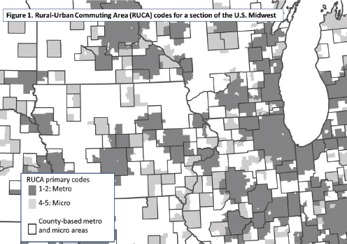
FIGURE B-1 Rural-Urban Commuting Area (RUCA) Codes for a section of the U.S. Midwest.
SOURCE: Prepared by John Cromartie for his presentation at Rationalizing Rural Area Classifications workshop. Based on USDA Economic Research Service data. See http://www.ers.usda.gov/data-products/rural-urban-commuting-areacodes.aspx [October 2015].
rural areas, as measured by relatively low commuting that fall within metro counties. RUCA Codes also identify those parts of nearby nonmetro counties that are highly connected to metro cores. The tract-based delimitation succeeds in identifying more precisely extent of micropolitan influence (shown in light gray), which in many cases does not include the entire county in which the core is located. In addition, the small size of census tracts allows for the identification of hundreds of smaller towns (with fewer than 10,000 people) and their local commuter sheds (not shown on map). The location and size of these much smaller spheres of economic influence cannot be detected with county-level classifications.
FRONTIER AND REMOTE CODES
The Frontier and Remote (FAR) Codes employ an increasingly popular, grid-based methodology in order to define proximity using travel time by car rather than by actual commuting flows. FAR areas are defined in relation to the time it takes to travel by car to the edges of nearby urbanized areas and urban clusters, which collectively are labeled urban areas (UAs). Travel time is measured at the ½ x ½ kilometer grid level, using routing algorithms applied to a road network that includes all federal, state, and county paved roads. The methodology departs significantly from the previous three classifications and the resulting classification focuses more exclusively on the far rural end of the urban-rural spectrum. However, the underlying concepts of urban size and proximity are the same.
The term “frontier and remote” is used here to describe territory characterized by some combination of low population size and a high degree of geographic remoteness. As with the RUCA Codes, demand for a geographically detailed delineation of frontier areas came from the Office of Rural Health Policy, to help administer HHS programs with the legislative mandate to improve access to health-care in frontier areas. Potential policy-relevant research applications spurred development of the FAR Codes as well. In the United States, remoteness has been linked with population loss and persistent net out-migration (Albrecht, 1993; Cromartie, 1998); an aging population and natural decrease (Johnson, 1993; Johnson and Rathge, 2006); and loss of retail and wholesale trade (Adamchak et al., 1999; Henderson, Kelly, and Taylor, 2000). In the late 2000s, research was beginning to show increased economic penalties associated with remoteness (Partridge et al., 2008, 2009).
A revival in research based on central place theory among economists, geographers, and regional scientists, following development of a New Economic Geography (Krugman, 1991), helped focus attention on unique issues facing remote areas. As described in an earlier article on the FAR Codes:
Perhaps the defining challenge facing frontier communities is the increased per capita cost of providing services. Health care costs are a primary policy issue motivating this research, but remoteness increases costs in accessing groceries, household goods, child care, entertainment, and all types of publically provided social services, such as schools or fire protection. According to central place theory, the costs associated with providing higher-order services (appliances, motor vehicles, major trauma intervention) are higher than those associated with lower-order services (groceries, sporting goods, nursing care), thus they require a larger population to support them (Mulligan, 1984). . . . [R]ecent studies
confirm that the variability of rural well-being is still very strongly tied to the structure of the urban hierarchy . . . (Cromartie, Nulph, and Hart, 2012).
In partnership with HHS, ERS created the first version of the FAR Codes in 2012, using 2000 Census data, then released a version in 2015 based on 2010 data. Four FAR levels were defined based on urban area size, with the notion that urban areas of different sizes offer different levels of services and different labor market opportunities. For each of 32.4 million grid cells, travel times to nearby UAs were examined and up to four pieces of information retained—the travel time in minutes to the edge of the nearest UA with a population in the following size ranges: 2,500-10,000, 10,000-24,999, 25,000-49,999, and 50,000 or more. These data allow for the four different FAR levels to be defined, based on adjusting the population size thresholds.
A key methodological innovation allowed with this approach is the ability to apply longer travel-time bands around larger UAs. The qualifying travel time (beyond which areas are considered to be frontier and remote) should be longer around larger UAs, because people tend to travel farther and less frequently for high-order services. For every grid cell, we calculate travel times to nearby UAs in the four population-size groups listed above, thus we can apply longer travel-time bands to larger population-size groups:
- Level 1—FAR areas consist of rural areas and urban areas up to 50,000 people that are 60 minutes or more from an urban area of 50,000 or more people.
- Level 2—FAR areas consist of rural areas and urban areas up to 25,000 people that are 45 minutes or more from an urban area of 25,000-49,999 people; and 60 minutes or more from an urban area of 50,000 or more people.
- Level 3—FAR areas consist of rural areas and urban areas up to 10,000 people that are 30 minutes or more from an urban area of 10,000-24,999; 45 minutes or more from an urban area of 25,000-49,999 people; and 60 minutes or more from an urban area of 50,000 or more people.
- Level 4—FAR areas consist of rural areas that are 15 minutes or more from an urban area of 2,500-9,999 people; 30 minutes or more from an urban area of 10,000-24,999 people; 45 minutes or more from an urban area of 25,000-49,999 people; and 60 minutes or more from an urban area of 50,000 or more people (see http://www.ere.usda.gov/data-products/frontier-and-remote-areacodes.aspx [November 2015].
A relatively large number of people live far from cities providing “high order” goods and services, such as advanced medical procedures, major household appliances, regional airport hubs, and professional sports franchises. Level 1 FAR Codes are meant to approximate remoteness from these types of activities, more likely to be present in urbanized areas of 50,000 or more residents. Driving times of more than one hour designate remoteness from centers of this size. A much smaller, but still significant, number of people find it hard to access “low order” goods and services, such as grocery stores, gas stations, and basic health care needs. Level 4 FAR Codes, defined as travel time from an urban cluster of 2,500 to 9,999 residents more closely coincide with this, much higher degree of remoteness. Here, a travel time of over 15 minutes is considered “remote.” Other types of goods and services—clothing stores, car dealerships, movie theaters—fall somewhere in between in terms of likely center size, approximated by levels 2 and 3.
Once frontier categories are determined for each grid cell, frontier populations may be aggregated to larger, more useful geographic units, such as ZIP Code areas. For each ZIP Code area, the percent of the population defined as frontier was calculated. For ZIP Code areas containing a mix of frontier and nonfrontier populations, classification was based on the status of the majority of the population. The same analysis can be repeated for census tracts, counties, or other geographic units.
True to its “frontier” name, FAR territory is predominantly found in the West, from the Great Plains to the Oregon-California coast, and including almost all of Alaska.8 This geographically detailed approach also identifies significant pockets of relatively high remoteness east of the Mississippi, such as in northern New England, the Upper Great Lakes, Appalachia, and the Deep South. Previous delineations of frontier areas, mostly relying on county-based methods, fail to identify many of these remote regions.9 U.S. populations living in ZIP Code areas designated as FAR ranged from 12.2 million for level one down to 2.3 million for level four in 2010. These populations constitute just 3.9 and 0.7 of the total U.S. population, respectively. However, the share of land area classified as frontier and remote ranged from 52 percent for level 1 down to 35 percent for level 4. The fact that over one-half of U.S. territory is inhabited by just 12.2 million residents suggests in itself the very unique economic circumstances facing these communities and individuals.
_______________________
8FAR maps are posted on the ERS website, see http://www.ers.usda.gov/data-products/frontier-and-remote-area-codes/documentation.aspx [November 2015].
9The Rural Assistance Center shows one such map and discusses alternative ways to define frontier areas, see https://www.raconline.org/topics/frontier [November 2015].
CONCLUSIONS
In reporting research results to USDA officials, ERS frequently aims to communicate an ongoing policy challenge: Rural America is diverse and complex. Not only do challenges such as job retention and service provision look different in rural than in urban areas, but they vary also within rural areas by measures of population size and remoteness. Since the 1970s, ERS has developed and maintained multilevel, geographic classifications to provide detailed measures of rurality and to assess the economic and social diversity of rural and small-town America. These classification schemes have also been used to determine eligibility for federal programs that assist rural areas.
Rural America is not just diverse and complex, but has rapidly evolved in the 40 years since the first county classification was introduced. In that time, urbanization reduced the rural share of population by more than a third, globalization and technology reshaped the rural economy, and immigration, aging, and amenity migration gave rural America a new demographic profile. The four classification systems that are the focus of this paper were developed independently, in different decades to address specific research agendas and policy needs. It’s now helpful to step back and evaluate the group as a whole in light of changing realities on the ground, changing research priorities, and the changing policy landscape.
The information revolution has brought new data, new geographies, and new methodologies into play. Together they provide opportunities to improve geographic classifications, as well as major challenges in choosing the best solutions. For instance, the FAR classification measures urban access and remoteness using ½ kilometer grid cells, improving geographical accuracy for many applications. At the same time, county-level classifications will continue to be needed given data requirements. ERS faces the challenge of maintaining conceptual consistency at different geographic scales.
ERS will draw on results from this conference to identify what considerations need to go into modifying existing rural-urban classifications developing new ones. Key questions include How many categories can they contain without being overly complex? What thresholds should be used? Can data products be provided for different geographic building blocks in a consistent way? Or Are there inherent differences introduced when moving from one geographic level to another?
Modifications to existing classifications or the introduction of new schemes face several, often contradictory, demands. Ideally, they would be
- useful in identifying socioeconomic variation as it is affected by size of place and urban proximity;
- useful to policy makers in evaluating programs and delineating eligibility;
- useful to a broad range of stakeholders by being relatively easy to use, containing a reasonably small number of categories with discernable criteria;
- based on conceptually sound methodology, including justifiable breakpoints; and
- consistent with OMB and Census Bureau definitions.
It will not be possible to satisfy all these needs perfectly, so tradeoffs need to be considered. The workshop demonstrated that the desire to ensure the future viability and usability of these ERS products is a widely shared concern.


