
A
Calculating the Benefits of Rooftop Runoff Capture Systems
This appendix presents the methods used (with examples) to evaluate the beneficial uses of roof runoff harvesting for irrigation of landscaped areas and for toilet flushing. The Source Loading and Management Model, WinSLAMM (Pitt, 1997), was used to calculate the benefits of harvesting stormwater for storage and later beneficial uses. The methods were previously used and described by Pitt et al. (2011, 2014). WinSLAMM is a continuous model that evaluates a long series of rains for an area. WinSLAMM1 is licensed for sale but is available free of charge to academic institutions. An evaluation license is also available to interested readers who wish to examine the model for a limited time. Input files used in this scenario analysis are available in the Academies’ Public Access Records Office.
For this report, WinSLAMM focused on the capture of rooftop runoff and use for turfgrass irrigation and toilet flushing, as described in Box 3-1. Different storage tank volumes were also evaluated. Average monthly (and daily) irrigation requirements were calculated by subtracting average monthly rainfall from 1995 to 1999 (1996-1999 for Lincoln, because of missing data) from average monthly evapotranspiration (ET) values. Then using WinSLAMM and the 5-year precipitation time series, if rainfall was insufficient to meet the irrigation demand, then supplemental irrigation was required. If available, then the supplemental irrigation was supplied by previously stored roof runoff water in storage tanks. Toilet flushing requirements were based on typical national indoor water uses (11 gpcd; see Box 3-1). The following is a summary of the main calculations and data used for these analyses.
WINSLAMM
WinSLAMM evaluates stormwater runoff volumes and pollutant loads under an array of stormwater management practices including rain barrels and water tanks, although the committee did not assess pollutants in this analysis (Pitt, 1987). Using local rain records, the model calculates runoff volumes and pollutant loadings for each rain from individual source areas within various land use categories and sums the results over a given area or land use. Examples of runoff source areas considered by the model include roofs, streets, sidewalks, parking areas, and landscaped areas, which each have different runoff coefficients based on the type of surface, slope, and soil properties (Pitt, 1987). Example land use categories include commercial, industrial, institutional, open space, residential, and freeway/highway. The committee’s scenario modeling exercise mainly focuses on roof runoff for small-scale stormwater harvesting and on land use runoff for larger scale stormwater harvesting.
Any length of rainfall record can be analyzed with WinSLAMM, from a single event to many decades. The rainfall files used in the committee’s calculations were developed from hourly rainfall data obtained from the National Oceanic and Atmospheric Administration (NOAA) rainfall stations as published on EarthInfo CD-ROMs.
DATA REQUIREMENTS AND SOURCES OF INFORMATION
WinSLAMM uses various sets of information in its calculations. The main data required for the analyses in this report included rain data for the six locations examined (from NOAA weather stations), runoff coefficients for the source areas for different land uses, and land development characteristics for the land uses in each area examined.
Rainfall Data
As noted in the report, six areas of the country were examined to represent a range of climatic conditions:
- Los Angeles, California, having a median rainfall of about 12 inches per year over the long-term record (17 inches average during the 5-year calculation period)
__________________
1 See http://winslamm.com.
- Seattle, Washington, having a median rainfall of about 37 inches of rainfall per year (42 inches average during the 5-year calculation period)
- Lincoln, Nebraska, having a median rainfall of about 26 inches of rainfall per year (28 inches average during the 4-year calculation period)
- Madison, Wisconsin, having a median rainfall of about 32 inches of rainfall per year (30 inches average during the 5-year calculation period)
- Birmingham, Alabama, having a median rainfall of about 54 inches of rainfall per year (50 inches average during the 5-year calculation period)
- Newark, New Jersey, having a median rainfall of about 43 inches of rainfall per year (44 inches average during the 5-year calculation period)
Most of the modeling calculations focused on recent 5 years of rainfall records (1995 through 1999 for all areas, except for Lincoln, where 1996 through 1999 rains were used due to many missing rains in the 1995 record).
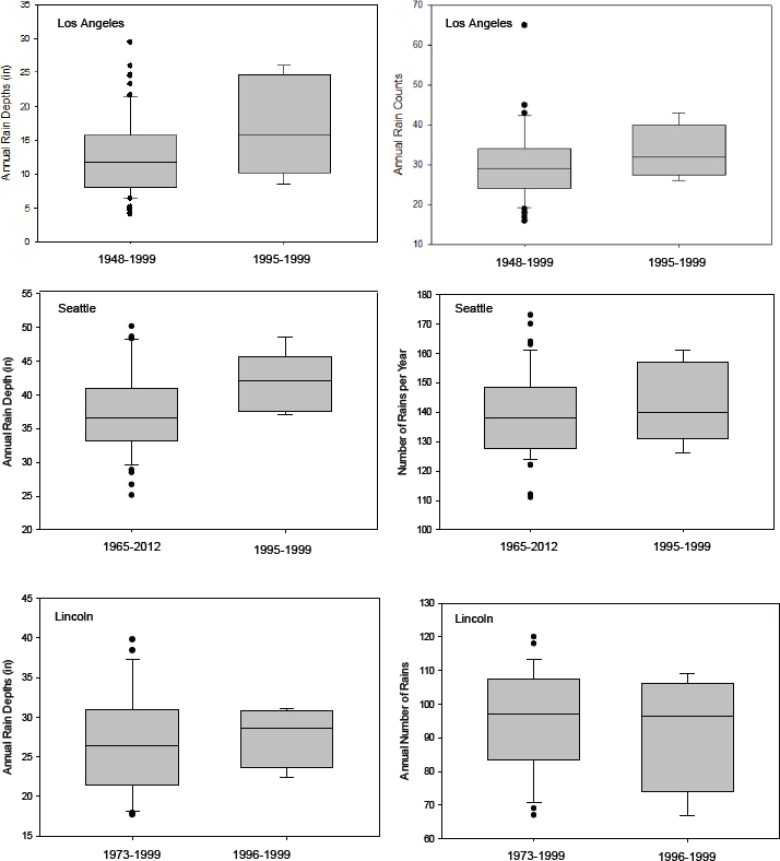
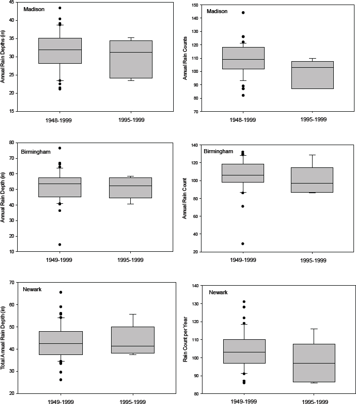
The goal was to use a continuous period of actual rains that were similar to the long-term average conditions, because continuous simulations were needed to calculate the inter-event water demands based on the average ET values. The committee based its scenario analysis on 5-year rain periods to reduce data pre-processing demands and because long records are rarely available without data gaps. Moderate rain record lengths reduce these gap problems (although Lincoln was missing 1995) and have been used to reduce large year-to-year variabilities while attempting to match the average monthly ET values. In Table A-1 and Figure A-1, the committee compares the rainfall data from the 4- to 5-year calculation periods with the long-term precipitation record. Some variations are apparent even though the differences are not statistically significant. Some of these differences are discussed in the context of analysis uncertainties in Box 3-2.
The committee judges that the calculation methods and data used for these analyses represent reasonable conditions and present results that are useful for the comparative analysis presented in Chapter 3. However, the data are not intended as definitive predictions or as a basis for design guidance.
TABLE A-1 Comparison of Precipitation Annual Rain Totals and Rain Counts Between the Scenario Analysis Calculation Period and the Long-term Rainfall Record
| Los Angeles, CA | Seattle, WA | Lincoln, NE | Madison, WI | Birmingham, AL | Newark, NJ | |
| Long-term rain record | 1948-1999 | 1965-2012 | 1973-1999 | 1948-1999 | 1948-1999 | 1948-1999 |
| (1995 gap) | (1978-1987 gap) | |||||
| Scenario analysis calculation | 1995-1999 | 1995-1999 | 1996-1999 | 1995-1999 | 1995-1999 | 1995-1999 |
| period | ||||||
| Long-term annual median | 11.70 | 36.69 | 26.45 | 31.85 | 53.68 | 42.51 |
| rain total (in) | ||||||
| Scenario analysis calc. period | 15.82 | 42.10 | 28.62 | 31.19 | 52.40 | 41.28 |
| median annual rain total (in) | ||||||
| p values (<0.05 indicatesa significant difference)a | 0.16 | 0.078 | 0.68 | 0.56 | 0.78 | 0.99 |
| Comment of rain depth box and whisker plot comparisons | The calculation period has greater rains and a wider variation than the long term conditions | The calculation period has greater rains but similar variations as the long term conditions | The calculation period has similar rain depths per year and the variations are similar | The calculation period has smaller rain depths per year and the variations are similar | The calculation period has similar rain depths per year and the variations are similar | The calculation period has similar rain depths per year and the variations are similar |
| Long-term annual median rain counts | 29 | 138 | 97 | 109 | 106 | 103 |
| Scenario analysis calc. period median annual rain counts | 32 | 140 | 97 | 103 | 97 | 97 |
| p values (<0.05 indicatesa significant difference)a | 0.27 | 0.62 | 0.82 | 0.08 | 0.20 | 0.17 |
aMann-Whitney rank sum p values (not independent data sets because the calculation period was included in the total period). Deemed acceptable as the hypothesis was to compare the full set with the subset. None of the rain depth or rain count comparisons indicated significant differences for the number of data available.
Land Development Characteristics
An important element in calculating stormwater beneficial use opportunities using harvested roof runoff for landscaping irrigation is to know the typical areas of the roofs and the landscaped areas that are present in the different land uses and study locations. For larger-scale beneficial-use calculations, the areas of the other source areas in the land uses also need to be known. These areas were obtained from prior summaries conducted to support the U.S. Environmental Protection Agency’s (EPA’s) development of potential future stormwater regulations. These typical land development characteristics throughout the country, described in Pitt (2011a,b,c), are summarized in Table 3-3. Pitt (2011a) contains the citations and sources for the original data sources. More than 100 monitored locations were reviewed using site mapping and aerial photographs, along with concurrent monitoring data.
For irrigation beneficial uses of stormwater, the most suitable source for the collected water is from the building roofs because of its generally better water quality, high unit area runoff yield, and elevation above storage tanks and irrigated land. The landscaped areas represent the amount of area that can be irrigated with the harvested roof runoff water. Therefore, areas having relatively large roofs and small landscaped areas are most likely to have most of the irrigation demand in the area satisfied (but may not reduce the overall stormwater discharges as much as areas having small roofs and large irrigable land). Table A-2 shows the roof and landscaped areas for these six land uses for the Los Angeles area. Commercial areas generally have the smallest ratios of landscaped to roof areas and therefore are more likely to be able to meet irrigation requirements with the abundance of roof runoff. In contrast, it would be much more challenging to replace much of the irrigation water currently supplied by potable water supplies using roof runoff in low-density areas because the amount of roof runoff water is a much smaller portion of the total irrigation requirements. There are some differences in these development characteristics by region, and the rainfall patterns and evapotranspiration requirements vary greatly by area. Table A-3 shows the percentage of landscaped and roof areas and typical housing densities for medium-density, residential land uses (the focus of the committee’s analysis) in each of the six locations of the country examined.
ROOF RUNOFF CALCULATIONS
The following sections describe an example set of calculations used to develop the analyses used in this report. These examples focus on medium-density, residential land use in Los Angeles.
TABLE A-2 Roof and Landscaped Areas for Los Angeles Land Uses
| Roof Area (%) | Landscaped Area (%) | Ratio of Landscaped Area to Roof Area | |
| Commercial | 28.1 | 14.9 | 0.53 |
| High-density residential | 20.7 | 46.4 | 2.24 |
| Medium-density residential | 18.0 | 52.5 | 2.92 |
| Low-density residential | 8.0 | 79.6 | 9.95 |
| Industrial | 20.2 | 24.3 | 1.20 |
| Institutional | 19.4 | 41.2 | 2.12 |
TABLE A-3 Landscaped and Roof Area, and Number of Households for Medium-Density, Residential Land Use in Six U.S. Locations
| Landscaped Areas (%) | Roof Areas (%) | # Roofs/100 Acres at 1,500 ft2 Each | |
| Los Angeles, CA | 52.5 | 18.0 | 523 |
| Seattle, WA | 63.5 | 17.1 | 497 |
| Lincoln, NE | 62.8 | 18.1 | 526 |
| Madison, WI | 63.3 | 15.0 | 436 |
| Birmingham, AL | 81.3 | 8.8 | 256 |
| Newark, NJ | 56.2 | 15.9 | 462 |
Runoff Quantity
Table A-4 is a small portion of the WinSLAMM modeled scenario output showing runoff volume contributions for a 100-acre medium-density residential area in Los Angeles. These analyses were repeated for six major land use areas (commercial, high-density residential, medium-density residential, low-density residential, industrial, and institutional) and six U.S. locations. During this 5-year period examined (1995-1999), a total of about 84 inches fell, with rains as large as 3.5 inches (Table A-5). About 47 percent of the rainfall occurred as direct runoff for this area (or a the volumetric runoff coefficient [Rv] of 0.47), higher than for most residential areas, because these analyses assumed directly connected roof drainage, as would be the case for roof runoff harvesting. Most of the runoff volumes in this medium-density residential land use analysis originated from the street and roof areas, with smaller (and about equal amounts) from driveways, sidewalks, and landscaped areas. These relationships vary for different land uses and different geographical areas based on the local development characteristics, soils, and rain patterns.
Based on the 1995-1999 period, 100 acres of medium-density, residential area in Los Angeles produces about 14 million ft3 of runoff, while the roofs in the area contribute about 5.2 million ft3 of that runoff. These can be converted to inches of runoff over the drainage area for the 5-year period, for example:
![]()
For the roof area alone (which comprises 18 percent of the land use, or 18 acres):
![]()
The total rain depth for the 5 years is 83.67 inches, or 16.73 inches per year. The volumetric runoff coefficient (Rv) is the ratio of the runoff total to the rain total. Therefore, for the whole area, the total flow-weighted annual Rv is:
![]()
while the Rv for the roof area alone is:
TABLE A-4 Portion of WinSLAMM Model Output for Southwest, Medium-Density, Residential Areas (100-acre area) Showing Runoff Amounts (ft3) from Different Sources Areas for Each Event and for All Areas Combined (5 years rain series)
Runoff Amounts (ft3) |
||||||||||
| Month | Start Date | Rain Total (in.) | Land Use Totals | Roofs | Driveways | Sidewalks/Walks | Street Area | Small Landscaped Area | Volumetric Runoff Coeff. (Rv) | Total Losses (in.) |
| 1 | 1/3/1995 | 0.75 | 119,655 | 46,952 | 13,767 | 8,850 | 44,408 | 5,677 | 0.44 | 0.42 |
| 1 | 1/4/1995 | 3.5 | 716,277 | 226,403 | 83,501 | 53,679 | 219,291 | 133,402 | 0.56 | 1.53 |
| 1 | 1/7/1995 | 1.29 | 217,432 | 82,603 | 27,004 | 17,360 | 77,546 | 12,920 | 0.46 | 0.69 |
| 1 | 1/8/1995 | 0.4 | 56,379 | 24,323 | 6,521 | 4,192 | 19,719 | 1,623 | 0.39 | 0.24 |
| 1 | 1/10/1995 | 2.93 | 595,083 | 189,532 | 68,824 | 44,244 | 180,806 | 111,677 | 0.56 | 1.29 |
| 1 | 1/11/1995 | 0.14 | 16,023 | 7,115 | 1,812 | 1,165 | 5,931 | 0 | 0.32 | 0.1 |
| 1 | 1/11/1995 | 0.4 | 56,379 | 24,323 | 6,521 | 4,192 | 19,719 | 1,623 | 0.39 | 0.24 |
| 1 | 1/14/1995 | 0.12 | 13,386 | 5,899 | 1,499 | 964 | 5,024 | 0 | 0.31 | 0.08 |
| 1 | 1/20/1995 | 0.16 | 18,776 | 8,397 | 2,144 | 1,378 | 6,858 | 0 | 0.32 | 0.11 |
| About 150 events between these two dates are not shown on this summary table | ||||||||||
| 4 | 4/11/1999 | 1.36 | 229,828 | 87,085 | 28,777 | 18,499 | 81,753 | 13,713 | 0.47 | 0.73 |
| 6 | 6/1/1999 | 0.52 | 77,811 | 32,034 | 8,880 | 5,709 | 28,535 | 2,653 | 0.41 | 0.31 |
| 6 | 6/2/1999 | 0.05 | 3,334 | 1,152 | 476 | 306 | 1,401 | 0 | 0.18 | 0.04 |
| 6 | 6/3/1999 | 0.02 | 314.4 | 166 | 90 | 58 | 0 | 0 | 0.04 | 0.02 |
| 11 | 11/8/1999 | 0.27 | 34,913 | 15,520 | 4,046 | 2,601 | 12,344 | 402 | 0.36 | 0.17 |
| 11 | 11/17/1999 | 0.01 | 78.6 | 41 | 23 | 15 | 0 | 0 | 0.02 | 0.01 |
TABLE A-5 Summary of All Events in 5-Year Rain Series in WinSLAMM Model Output for Southwest, Medium-Density, Residential Areas (100 acre area)
| Rain Total (in.) |
Runoff Amounts (ft3) |
Volumetric Runoff Coeff. (Rv) | Total Losses (in.) | ||||||||||
| Land Use Totals | Roofs | Driveways | Sidewalks/ Walks | Street Area | Small Landscaped Area | ||||||||
| Minimum | 0.01 | 79 | 41 | 23 | 15 | 0 | 0 | 0.02 | 0.01 | ||||
| Maximum | 3.5 | 716,277 | 226,403 | 83,501 | 53,679 | 219,291 | 133,402 | 0.56 | 1.53 | ||||
| Average | 0.51 | 85,703 | 31,728 | 10,152 | 6,527 | 29,112 | 8,184 | 0.47 | 0.75 | ||||
| Total | 83.67 | 13,969,610 | 5,170,000 | 1,655,000 | 1,064,000 | 4,745,000 | 1,334,000 | n/a | 45.18 | ||||
TABLE A-6 Overall Summary of Runoff Volume Contributions by Source Area and Month for Los Angeles Medium Density Residential Areas
| Five-Year Average Flows by Month | Rain Total (in.) | Land Use Totals | Roofs | Driveways | Sidewalks/ Walks | Street Area | Small Landscaped Area |
| Area (% of total land use) | n/a | 100.00 | 18.00 | 7.00 | 4.50 | 18.00 | 52.50 |
| Avg Jan runoff volume (in/mo) | 4.89 | 2.26 | 4.65 | 3.85 | 3.85 | 4.26 | 0.41 |
| Avg Feb runoff volume (in/mo) | 3.76 | 1.88 | 3.63 | 3.13 | 3.13 | 3.38 | 0.49 |
| Avg March runoff volume (in/mo) | 2.48 | 1.13 | 2.33 | 1.88 | 1.88 | 2.12 | 0.22 |
| Avg April runoff volume (in/mo) | 0.86 | 0.35 | 0.78 | 0.60 | 0.60 | 0.70 | 0.03 |
| Avg May runoff volume (in/mo) | 0.59 | 0.24 | 0.54 | 0.42 | 0.42 | 0.49 | 0.02 |
| Avg June runoff volume (in/mo) | 0.25 | 0.09 | 0.21 | 0.15 | 0.15 | 0.18 | 0.00 |
| Avg July runoff volume (in/mo) | 0.01 | 0.00 | 0.01 | 0.00 | 0.00 | 0.01 | 0.00 |
| Avg Aug runoff volume (in/mo) | 0.00 | 0.00 | 0.00 | 0.00 | 0.00 | 0.00 | 0.00 |
| Avg Sept runoff volume (in/mo) | 0.05 | 0.02 | 0.05 | 0.03 | 0.03 | 0.04 | 0.00 |
| Avg Oct runoff volume (in/mo) | 0.29 | 0.13 | 0.28 | 0.24 | 0.24 | 0.26 | 0.02 |
| Avg Nov runoff volume (in/mo) | 1.30 | 0.56 | 1.22 | 0.95 | 0.95 | 1.11 | 0.05 |
| Avg Dec runoff volume (in/mo) | 2.24 | 1.03 | 2.14 | 1.77 | 1.77 | 1.97 | 0.16 |
All of the event data were sorted by month and then averaged to develop 5-year averaged monthly summaries of runoff volumes (average inches of runoff per month). Table A-6 is an overall summary showing these runoff volume contributions from each of the Los Angeles, medium-density, residential, source areas and the total annual flow conditions, expressed in average watershed-inches per month.
Evapotranspiration and Irrigation Demands
Evapotranspiration (ET) is defined as the rate at which readily available water is removed from the soil and plant surfaces, expressed as the rate of latent heat transfer per unit area or as a depth of water evaporated and transpired from a reference crop (Jensen et al., 1990). In the United States, ET monitoring is primarily focused in agricultural and wild land environments. With educational advancements stressing water conservation in urban areas, there is a new desire to apply ET data as a part of stormwater harvesting options for supplemental irrigation and to fine-tune actual irrigation requirements based on soil moisture and plant needs. Climate-based equations are the most common method used to determine ET. ET potential, ETo, is only relevant for a standard condition that reflects normalized agricultural conditions. The ETo value is therefore adjusted according to the microclimate, soils, plants, and growing season conditions. Most of these adjustment factors were developed for agricultural situations, and their use in highly disturbed urban environments has not been well documented. However, it is becoming more common to directly measure urban area ET as part of stormwater management projects. As an example, Selbig and Balster (2010) directly measured ET in an urban setting in Madison, Wisconsin, as part of a stormwater management project for a variety of soil and plant conditions, including when the plants were mostly covered with snow.
The California Irrigation Management Information System (CIMIS) is a comprehensive example for determining ET rates within a state. Its web services are capable of pro-
ducing an array of useful information about most locations and regions in California. The stations monitored are not limited to traditional agricultural areas, with some monitoring data also available in urban areas.
The ASCE Standardized Reference Equation (Allen et al., 2005) is an example of an ET equation that has been adopted for reference ETo calculations. Both the ASCE and Food and Agriculture Organization (FAO-56) have approved versions of the equation with only minor differences (standard crop height being the major difference). ASCE reference ETo can be calculated for only two specific crop heights—short (grasses) and tall (alfalfa). The data used in this report were calculated for a short reference crop, most relevant to typical home lawns.
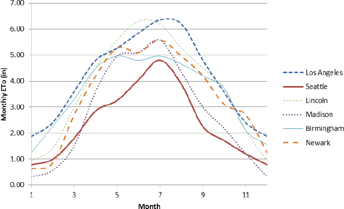
The monthly rainfalls (or soil moisture additions due to the rainfall) for each geographical area, expressed in inches/ month, were compared to the evapotranspiration rate requirements for landscaped area plants to determine the irrigation requirements to meet the plant’s minimum moisture needs. The reference evapotranspiration rates (ETo) were obtained from CIMIS for the southwest near Los Angeles and from the ASCE standardized reference equations for the other locations, as shown on Table A-7. The ETo values are given in inches/day and were therefore converted to inches/month for direct comparison to the monthly rainfall (or soil moisture addition) values. The Los Angeles and Seattle rainfall monitoring locations were represented by two ETo stations that were averaged for these analyses. The other areas only had single ETo stations representing their rainfall monitoring locations. Table A-8 shows the monthly values, while Figure A-2 is a plot comparing the seasonal evapotranspiration values for these six rainfall monitoring locations. The ETo patterns are similar for all locations with the greatest values (maximums of about 5 to 6.5 inches/month) occurring in the summer months, while the minimum winter ETo values are less than 2 inches/month. Seattle has the lowest ETo values for most months (annual total of about 28 inches), while Los Angeles has the highest values for most months (annual total of about 49 inches). Specific details on modeling evapotranspiration are also given by Pitt, et al. (2008).
Tables A-9 through A-14, along with Figure 3-2, show the calculations and resulting plots indicating the average monthly irrigation requirements (based on 1995-1999 rainfall; 1995-1999 for Lincoln) to meet the long-term average monthly ET values. A plant’s actual ET is calculated by multiplying ETo rates by coefficients for each plant type providing a daily moisture estimate for the crop under well-watered conditions. Romero and Dukes (2008) prepared a summary of crop coefficients for the Southwest Florida Water Management District and the Florida Agricultural Experiment Station, which lists turfgrass coefficients for warm and humid areas that ranged from about 0.55 to 0.79 for warm
TABLE A-7 Evapotranspiration Reference Rate (ETo) Stations Used for Beneficial Use Calculations
| Rain Gage Location | ETo Data Source | Station Name | Latitude | Longitude | Elev. (ft) |
| Los Angeles Airport Weather Service Office, CA | CIMIS Average Monthly Rates, 1989-2011 | Glendale, CA | 34.197 | -118.230 | 1,111 |
| Long Beach, CA | 33.799 | -118.095 | 17 | ||
| Seattle Tacoma Airport, WA | ASCE Std. Ref. Eq., 2005-2010 | Quilcene, WA | 47.82 | -122.88 | 62 |
| Enumclaw, WA | 47.2 | -121.96 | 771 | ||
| Lincoln Airport, NE | ASCE Std. Ref. Eq., 2008-2011 | Rainwater Basin NE | 40.57 | -98.17 | 1,790 |
| Madison Dane Co Airport, WI | ASCE Std. Ref. Eq., 2005-2011 | Wautoma, WI | 43.1 | -89.333 | 857 |
| Birmingham Airport, AL | ASCE Std. Ref. Eq., 2003-2011 | Talladega, AL | 33.44 | -86.081 | 600 |
| Newark International Airport, NJ | ASCE Std. Ref. Eq., 2005-2011 | New Middlesex County NJ | 40.41 | -74.494 | 116 |
TABLE A-8 Monthly ETo Values for Study Locations (inches/month)
| Jan | Feb | March | April | May | June | July | Aug | Sept | Oct | Nov | Dec | Annual total (inches/yr) | |
| Los Angeles, CA | 1.86 | 2.40 | 3.60 | 4.80 | 5.27 | 5.85 | 6.36 | 6.20 | 4.80 | 3.57 | 2.40 | 1.86 | 48.96 |
| Seattle, WA | 0.78 | 0.99 | 1.80 | 2.85 | 3.26 | 4.05 | 4.81 | 3.88 | 2.25 | 1.71 | 1.20 | 0.78 | 28.33 |
| Lincoln, NE | 0.93 | 1.41 | 3.00 | 4.50 | 5.58 | 6.30 | 6.20 | 5.27 | 4.50 | 3.72 | 2.10 | 0.93 | 44.44 |
| Madison, WI | 0.31 | 0.57 | 1.50 | 3.60 | 4.96 | 5.10 | 5.58 | 4.34 | 3.00 | 2.17 | 1.20 | 0.31 | 32.64 |
| Birmingham, AL | 1.24 | 2.26 | 3.30 | 4.50 | 4.96 | 4.80 | 4.96 | 4.65 | 4.20 | 3.72 | 2.10 | 1.55 | 42.24 |
| Newark, NJ | 0.62 | 0.85 | 2.70 | 4.20 | 5.27 | 5.10 | 5.58 | 4.96 | 4.20 | 3.10 | 2.70 | 1.24 | 40.52 |
season grasses. Aronson et al. (1987) listed coefficients for cool season grasses in the humid Northeast that ranged from about 0.6 to 1.04. Brown et al. (2001) presented a summary for arid areas with turfgrass coefficients ranging from about 0.8 to 0.9. For the calculations in this report, a turfgrass coefficient of 0.8 was used for all conditions.
Tables A-9 through A-14 show the monthly ETo reference values, the 0.8 turf grass coefficient that reduces the reference ETo values to obtain the actual expected evapotranspiration for typical turf grass, along with the average monthly rainfall amounts (based on 1995-1999 precipitation data for five locations and 1996-1999 data for Lincoln). The irrigation requirements shown here are simply the average amounts of water needed monthly in addition to rainfall to meet the ET requirements. Other calculations also considered the moisture added to the soil for each rain instead of the total rainfall, because not all of the rain infiltrates and is available for the plants. These tables show the actual differences between the average ET and rainfall values, and some (especially in the wetter months, or months having low ET requirements) have negative values (the rainfall is greater than the ET requirements). The actual average irrigation requirements per month ignore these negative values, as months with excessive rainfall cannot benefit months requiring irrigation, unless the excess runoff is stored for later beneficial uses (as indicated below in the storage tank modeling descriptions). Figure 3-2 graphically illustrates the average monthly irrigation requirements for the landscaped areas for each of these locations, which were then used in the model to calculate the effects of storage and roof runoff volumes for the different land uses on the resulting domestic water savings.
Table A-15 shows the amount of landscaped area as a percentage of the total land use for different areas in the Los Angeles. The monthly irrigation needs in ft3 of water per acre of land use per month was calculated by unit conversions using the landscaped area percentage of the land use and the irrigation requirements in inches/month. Small rounding effects may be reflected in the summary tables and example calculations because the model and spreadsheet calculations are high precision, while the summaries and example calculations used truncated significant digits. Also shown on Table A-15 are the total runoff amounts from the roofs and for the whole area for these land uses in Los Angeles. Except for the commercial and industrial areas, land use runoff is not sufficient to completely satisfy the irrigation requirements, and roof runoff alone is close to meeting the irrigation needs only for the commercial areas (simply on a total volume comparison, assuming sufficient storage is provided). The effects of storage tanks also need to be considered, as described below. Other geographical areas with differing rain and ET patterns, plus different land development characteristics, result in dif-
ferent conclusions. Table A-16 shows the irrigation requirement, expressed in gallons per day per 100 acres of the land use, as used by the model as the water demand for three of the six locations analyzed.
Domestic Water Savings Due to Roof Runoff Harvesting
Two volumes corresponding to typical water storage scenarios (two water barrels per household and one large water storage tank per household) were examined with WinSLAMM corresponding to typical runoff harvesting scenarios. Table A-17 shows the storage volume calculations for the two water storage tank options examined, shown for the Los Angeles example. The model calculates the stormwater runoff volume reductions using continuous simulations for the study period. The water storage tanks are continuously modeled based on additions of roof runoff for each rain and withdrawals to meet monthly average irrigation demand to meet the ET deficits, considering rainfall-induced changes in soil moisture. Overall indoor and outdoor water use behavior was assumed to be the unchanged with the addition of low-cost onsite sources of water. If the tank is full while runoff is still occurring, then the excess runoff is discharged to the drainage system and is not available for beneficial use. If the tank empties due to water withdrawals, then supplemental potable water would be needed to meet additional water demands. Small tanks overflow and are empty more frequently than larger tanks and therefore supply less water for beneficial uses.
The Los Angeles water savings are calculated based on the runoff reductions (with 153,731 ft3 of water storage volume per 100 acres, corresponding to a single 2,200-gallon water tank at each home). The model calculated 11.6 percent stormwater runoff reductions using this size tank for irrigation in this medium-density, residential land use area. The total average annual runoff for the medium-density, residential area was also calculated to be 27,940 ft3 per acre. The average domestic water savings by using harvested roof runoff for this scenario analysis is therefore:
![]()
or 2.42 millions of gallons (Mgal) per year for 100 acres.
Indoor Use of Roof Runoff for Toilet Flushing for Medium Density Residential Areas
Toilet flushing water use is based on a per capita water use of 11 gallons per capita per day. With 12 persons/acre and 100 acres of area, this is therefore
![]()
TABLE A-9 Los Angeles Irrigation Requirements to Meet ET Deficit
| Jan | Feb | Mar | Apr | May | Jun | Jul | Aug | Sept | Oct | Nov | Dec | Annual | |
| LA ETo, in/mo (reference) | 1.86 | 2.405 | 3.6 | 4.8 | 5.27 | 5.85 | 6.355 | 6.2 | 4.8 | 3.565 | 2.4 | 1.86 | |
| Turf grass coefficient | 0.8 | 0.8 | 0.8 | 0.8 | 0.8 | 0.8 | 0.8 | 0.8 | 0.8 | 0.8 | 0.8 | 0.8 | |
| LA ET, in/mo (corrected for turf grass) | 1.488 | 1.921 | 2.88 | 3.84 | 4.216 | 4.68 | 5.084 | 4.96 | 3.84 | 2.852 | 1.92 | 1.488 | 39.169 |
| LA avg rainfall (in/mo) | 4.89 | 3.76 | 2.48 | 0.86 | 0.59 | 0.25 | 0.01 | 0.00 | 0.05 | 0.29 | 1.30 | 2.24 | 16.734 |
| LA irrigation requirements to match | -3.406 | -1.837 | 0.4 | 2.976 | 3.622 | 4.434 | 5.072 | 4.96 | 3.788 | 2.562 | 0.616 | -0.752 | |
| ET (in/mo) | |||||||||||||
| LA irrigation requirements, ignoring excessive rainfall periods (in/mo) | 0 | 0 | 0.4 | 2.976 | 3.622 | 4.434 | 5.072 | 4.96 | 3.788 | 2.562 | 0.616 | 0 | 28.43 |
TABLE A-10 Seattle Irrigation Requirements to Meet ET Deficit
| Jan | Feb | Mar | Apr | May | Jun | Jul | Aug | Sept | Oct | Nov | Dec | Annual | |
| Seattle ETo, in/mo (reference) | 0.775 | 0.989 | 1.8 | 2.85 | 3.255 | 4.05 | 4.805 | 3.875 | 2.25 | 1.705 | 1.2 | 0.775 | |
| Turf grass coefficient | 0.8 | 0.8 | 0.8 | 0.8 | 0.8 | 0.8 | 0.8 | 0.8 | 0.8 | 0.8 | 0.8 | 0.8 | |
| SeaTac ET, in/mo (corrected for turf grass) | 0.62 | 0.791 | 1.44 | 2.28 | 2.604 | 3.24 | 3.844 | 3.1 | 1.8 | 1.364 | 0.96 | 0.62 | 22.663 |
| SeaTac avg rainfall (in/mo) | 6.20 | 5.12 | 4.05 | 2.63 | 1.28 | 1.21 | 0.78 | 1.06 | 1.24 | 4.00 | 7.92 | 6.22 | 41.694 |
| SeaTac irrigation requirements to match ET (in/mo) | -5.576 | -4.327 | -2.612 | -0.348 | 1.328 | 2.034 | 3.064 | 2.044 | 0.556 | -2.632 | -6.964 | -5.598 | |
| SeaTac irrigation requirements, ignoring excessive rainfall periods (in/mo) | 0 | 0 | 0 | 0 | 1.328 | 2.034 | 3.064 | 2.044 | 0.556 | 0 | 0 | 0 | 9.026 |
For a year and 100 acres, this amounts to 4.82 Mgal/yr. The indoor per capita water use and population density values were assumed to be the same for all of the medium-density, residential areas examined.
Table A-18 summarizes the monthly Los Angeles water uses for the three water demand scenarios examined in the report: conservation irrigation, toilet flushing, and conservation irrigation plus toilet flushing combined. Table A-19 shows the calculated potential water savings from the WinSLAMM model for the 5 years of rainfall data in a Los Angeles, 100-acre, medium-density, residential, study area. Values were obtained for both the roof areas alone and the total area to check the water savings values. The model calculations for water savings were averaged to obtain the annual runoff savings in both ft3 and millions of gallons.
VERIFICATION OF ORIGINAL ANALYSIS
The committee performed several levels of verification on this original analysis of water savings potential to ensure that the results are sound. The committee members performing the analysis vetted the assumptions of the analysis with
TABLE A-11 Lincoln Irrigation Requirements to Meet ET Deficit
| Jan | Feb | Mar | Apr | May | Jun | Jul | Aug | Sept | Oct | Nov | Dec | Annual | |
| Lincoln ETo, in/mo (reference) | 0.93 | 1.4125 | 3 | 4.5 | 5.58 | 6.3 | 6.2 | 5.27 | 4.5 | 3.72 | 2.1 | 0.93 | |
| Turf grass coefficient | 0.8 | 0.8 | 0.8 | 0.8 | 0.8 | 0.8 | 0.8 | 0.8 | 0.8 | 0.8 | 0.8 | 0.8 | |
| Lincoln ET, in/mo (corrected for turf grass) | 0.744 | 1.13 | 2.4 | 3.6 | 4.464 | 5.04 | 4.96 | 4.216 | 3.6 | 2.976 | 1.68 | 0.744 | 35.554 |
| Lincoln avg rainfall (in/mo) | 0.58 | 0.55 | 1.47 | 3.19 | 5.29 | 4.30 | 2.44 | 3.89 | 1.82 | 1.69 | 2.15 | 0.31 | 27.675 |
| Lincoln irrigation requirements to match ET (in/mo) | 0.1665 | 0.5775 | 0.935 | 0.4075 | -0.826 | 0.7425 | 2.52 | 0.326 | 1.78 | 1.286 | -0.47 | 0.434 | |
| Lincoln irrigation requirements, ignoring excessive rainfall periods (in/mo) | 0.1665 | 0.5775 | 0.935 | 0.4075 | 0 | 0.7425 | 2.52 | 0.326 | 1.78 | 1.286 | 0 | 0.434 | 9.175 |
TABLE A-12 Madison Irrigation Requirements to Meet ET Deficit
| Jan | Feb | Mar | Apr | May | Jun | Jul | Aug | Sept | Oct | Nov | Dec | Annual | |
| Madison ETo, in/mo (reference) | 0.31 | 0.565 | 1.5 | 3.6 | 4.96 | 5.1 | 5.58 | 4.34 | 3 | 2.17 | 1.2 | 0.31 | |
| Turf grass coefficient | 0.8 | 0.8 | 0.8 | 0.8 | 0.8 | 0.8 | 0.8 | 0.8 | 0.8 | 0.8 | 0.8 | 0.8 | |
| Madison ET, in/mo (corrected for turf grass) | 0.248 | 0.452 | 1.2 | 2.88 | 3.968 | 4.08 | 4.464 | 3.472 | 2.4 | 1.736 | 0.96 | 0.248 | 26.108 |
| Madison avg rainfall (in/mo) | 1.49 | 0.83 | 1.81 | 3.46 | 3.13 | 5.55 | 4.07 | 3.18 | 1.59 | 2.60 | 1.33 | 0.59 | 29.62 |
| Madison irrigation requirements to match ET (in/mo) | -1.244 | -0.378 | -0.614 | -0.576 | 0.842 | -1.47 | 0.394 | 0.288 | 0.812 | -0.86 | -0.368 | -0.338 | |
| Madison irrigation requirements, ignoring excessive rainfall periods (in/mo) | 0 | 0 | 0 | 0 | 0.842 | 0 | 0.394 | 0.288 | 0.812 | 0 | 0 | 0 | 2.336 |
TABLE A-13 Birmingham Irrigation Requirements to Meet ET Deficit
| Jan | Feb | Mar | Apr | May | Jun | Jul | Aug | Sept | Oct | Nov | Dec | Annual | |
| Birmingham ETo, in/mo (reference) | 1.24 | 2.26 | 3.3 | 4.5 | 4.96 | 4.8 | 4.96 | 4.65 | 4.2 | 3.72 | 2.1 | 1.55 | |
| Turf grass coefficient | 0.8 | 0.8 | 0.8 | 0.8 | 0.8 | 0.8 | 0.8 | 0.8 | 0.8 | 0.8 | 0.8 | 0.8 | |
| Birmingham ET, in/mo (corrected for turf grass) | 0.992 | 1.808 | 2.64 | 3.6 | 3.968 | 3.84 | 3.968 | 3.72 | 3.36 | 2.976 | 1.68 | 1.24 | 33.792 |
| Birmingham avg rainfall (in/mo) | 6.88 | 4.32 | 5.96 | 4.26 | 3.96 | 2.66 | 3.86 | 3.36 | 3.12 | 4.92 | 3.72 | 2.82 | 49.84 |
| Birmingham irrigation requirements to match ET (in/mo) | -5.888 | -2.512 | -3.32 | -0.66 | 0.008 | 1.18 | 0.108 | 0.36 | 0.24 | -1.944 | -2.04 | -1.58 | |
| Birmingham irrigation requirements, ignoring excessive rainfall periods (in/mo) | 0 | 0 | 0 | 0 | 0.008 | 1.18 | 0.108 | 0.36 | 0.24 | 0 | 0 | 0 | 1.896 |
TABLE A-14 Newark Irrigation Requirements to Meet ET Deficit
| Jan | Feb | Mar | Apr | May | Jun | Jul | Aug | Sept | Oct | Nov | Dec | Annual | |
| Newark ETo, in/mo (reference) | 0.62 | 0.8475 | 2.7 | 4.2 | 5.27 | 5.1 | 5.58 | 4.96 | 4.2 | 3.1 | 2.7 | 1.24 | |
| Turf grass coefficient | 0.8 | 0.8 | 0.8 | 0.8 | 0.8 | 0.8 | 0.8 | 0.8 | 0.8 | 0.8 | 0.8 | 0.8 | |
| Newark ET, in/mo (corrected for turf grass) | 0.496 | 0.678 | 2.16 | 3.36 | 4.216 | 4.08 | 4.464 | 3.968 | 3.36 | 2.48 | 2.16 | 0.992 | 32.414 |
| Newark avg rainfall (in/mo) | 4.56 | 3.07 | 3.71 | 3.70 | 3.89 | 2.94 | 4.30 | 2.65 | 4.65 | 3.60 | 3.58 | 2.86 | 43.514 |
| Newark irrigation requirements to match ET (in/mo) | -4.06 | -2.388 | -1.554 | -0.336 | 0.328 | 1.14 | 0.16 | 1.32 | -1.292 | -1.122 | -1.424 | -1.872 | |
| Newark irrigation requirements, ignoring excessive rainfall periods (in/mo) | 0 | 0 | 0 | 0 | 0.328 | 1.14 | 0.16 | 1.32 | 0 | 0 | 0 | 0 | 2.948 |
TABLE A-15 Example Watershed Demand and Available Stormwater by Land Use in Los Angeles
| Landscaped Area (% of total land use) | ft3 of irrigation water/acre/mo | Total Annual Irrigation Demand to Meet ET (ft3/acre) | Total Annual Roof Runoff (ft3/acre) | Total Annual Land Use Runoff (ft3/acre) | ||||||||||||
| Jan | Feb | March | April | May | June | July | Aug | Sept | Oct | Nov | Dec | |||||
| Commercial | 14.9 | 0 | 0 | 216 | 1,610 | 1,959 | 2,398 | 2,743 | 2,683 | 2,049 | 1,386 | 333 | 0 | 15,377 | 14,014 | 42,822 |
| High density residential | 46.4 | 0 | 0 | 674 | 5,013 | 6,101 | 7,468 | 8,543 | 8,354 | 6,380 | 4,315 | 1,038 | 0 | 47,885 | 11,894 | 30,603 |
| Medium densit residential | 52.5 | 0 | 0 | 762 | 5,672 | 6,903 | 8,450 | 9,666 | 9,453 | 7,219 | 4,883 | 1,174 | 0 | 54,180 | 10,344 | 27,939 |
| Low density residential | 79.6 | 0 | 0 | 1,156 | 8,599 | 10,466 | 12,812 | 14,655 | 14,332 | 10,945 | 7,403 | 1,780 | 0 | 82,148 | 4,596 | 14,892 |
| Industrial | 24.3 | 0 | 0 | 353 | 2,625 | 3,195 | 3,911 | 4,474 | 4,375 | 3,341 | 2,260 | 543 | 0 | 25,078 | 10,074 | 33,534 |
| Institutional | 41.2 | 0 | 0 | 598 | 4,451 | 5,417 | 6,631 | 7,585 | 7,418 | 5,665 | 3,832 | 921 | 0 | 42,519 | 9,676 | 30,920 |
TABLE A-16 Example Irrigation Demand for Land Uses in the Los Angeles, Lincoln, and Newark (gal/day per 100 acres of land use area)
| gal/day per 100 Acres of Land Use for Tank Modeling | Roof area (%) | Jan | Feb | Mar | Apr | May | Jun | Jul | Aug | Sept | Oct | Nov | Dec |
| Los Angeles commercial | 28.1 | 0 | 0 | 5,323 | 39,605 | 48,202 | 59,009 | 67,499 | 66,009 | 50,412 | 34,096 | 8,198 | 0 |
| Los Angeles high density residential | 20.7 | 0 | 0 | 16,577 | 123,335 | 150,107 | 183,759 | 210,200 | 205,558 | 156,987 | 106,177 | 25,529 | 0 |
| Los Angeles med. density residential | 18.0 | 0 | 0 | 18,406 | 141,504 | 166,665 | 210,830 | 233,386 | 228,233 | 180,114 | 117,890 | 29,290 | 0 |
| Los Angeles low density residential | 8 | 0 | 0 | 28,439 | 211,583 | 257,511 | 315,242 | 360,601 | 352,638 | 269,313 | 182,149 | 43,795 | 0 |
| Los Angeles industrial | 20.2 | 0 | 0 | 8,682 | 64,591 | 78,612 | 96,236 | 110,083 | 107,652 | 82,215 | 55,606 | 13,370 | 0 |
| Los Angeles institutional | 19.4 | 0 | 0 | 14,719 | 109,513 | 133,285 | 163,165 | 186,643 | 182,521 | 139,393 | 94,278 | 22,668 | 0 |
| Lincoln commercial | 25.0 | 2,082 | 7,221 | 11,692 | 5,096 | 0 | 9,285 | 31,230 | 3,420 | 22,258 | 15,393 | 0 | 5,271 |
| Lincoln high density residential | 20.7 | 6,900 | 23,933 | 38,749 | 16,888 | 0 | 30,772 | 103,504 | 11,335 | 73,769 | 51,017 | 0 | 17,468 |
| Lincoln medium density residential | 18.1 | 9,165 | 34,878 | 51,465 | 23,177 | 0 | 42,231 | 138,707 | 17,944 | 101,241 | 70,784 | 0 | 23,888 |
| Lincoln medium density residential | 18.1 | 9,339 | 32,393 | 52,445 | 22,857 | 0 | 41,648 | 140,088 | 15,341 | 99,842 | 69,048 | 0 | 23,642 |
| Lincoln low density residential | 14.9 | 9,830 | 34,095 | 55,201 | 24,058 | 0 | 43,836 | 147,449 | 16,147 | 105,089 | 72,677 | 0 | 24,885 |
| Lincoln industrial | 10.2 | 2,275 | 7,892 | 12,777 | 5,569 | 0 | 10,147 | 34,130 | 3,738 | 24,325 | 16,822 | 0 | 5,760 |
| Lincoln institutional | 24 | 6,469 | 22,438 | 36,327 | 15,833 | 0 | 28,848 | 97,035 | 10,626 | 69,158 | 47,828 | 0 | 16,377 |
| Newark commercial | 28.1 | 0 | 0 | 0 | 0 | 4,365 | 15,171 | 2,129 | 17,567 | 0 | 0 | 0 | 0 |
| Newark high density residential | 20.7 | 0 | 0 | 0 | 0 | 13,593 | 47,245 | 6,631 | 54,705 | 0 | 0 | 0 | 0 |
| Newark medium density residential | 15.9 | 0 | 0 | 0 | 0 | 16,464 | 57,224 | 8,031 | 66,259 | 0 | 0 | 0 | 0 |
| Newark low density residential | 8.0 | 0 | 0 | 0 | 0 | 23,320 | 81,050 | 11,375 | 93,847 | 0 | 0 | 0 | 0 |
| Newark industrial | 20.2 | 0 | 0 | 0 | 0 | 7,119 | 24,743 | 3,473 | 28,649 | 0 | 0 | 0 | 0 |
| Newark institutional | 19.4 | 0 | 0 | 0 | 0 | 12,070 | 41,950 | 5,888 | 48,574 | 0 | 0 | 0 | 0 |
the entire committee. Once the analysis was completed, two committee members and one staff person reviewed the spreadsheets containing the graywater analysis and the pre- and post-processing of the stormwater model analysis in detail to check for errors. Assumptions between the two analyses were compared for consistency, and a cell-by-cell assessment was performed to check that the appropriate values and formulas were used. Following this verification, a few minor errors that were detected were discussed with the staff and committee members responsible for the analysis and subsequently corrected.
Additionally, the analysis (including Chapter 3, Appendix A, and associated spreadsheets and input files) was sent to two independent unpaid consultants who were familiar with stormwater modeling to review. They were asked to assess whether the analysis and related assumptions were reasonable and appropriate and to identify any concerns or errors in the analysis. Feedback from the independent consultants was used to strengthen the discussion of uncertainties and the appropriate use of the scenario analysis findings.
TABLE A-17 Site Characteristics and Storage Volumes for the Los Angeles Example
| Parameter | Calculation |
| Roof area (ac per 100 ac of medium-density residential land uses, MDR) | 18% of 100 acres = 18 acres |
| Number of homes in 100 acres (1500 ft2 roof) |
|
| Rain barrel storage (gallons/100 ac) |
|
| Rain barrel storage (ft3/100 ac) |
|
| Rain barrel storage (ft3/ft2 roof area) |
|
| Water tank storage (gallons/100 ac) |
|
| Water tank storage (ft3/100 ac) |
|
| Water tank storage (ft3/ft2 roof area) |
|
| Landscaped area (ac per 100 ac of MDR) | 52.5% of 100 acres = 52.5 acres |
TABLE A-18 Average Monthly Water Use Patterns for Los Angeles Scenario
| Gallons/day/100 ac Medium-Density Residential (MDR) Area | Southwest Minimum Irrigation Requirements (gal/day) | Southwest Toilet Flushing (gal/day) | Southwest Minimum Irrigation Plus Toilet Flushing (gal/day) |
| Jan | 0 | 13,200 | 13,200 |
| Feb | 0 | 13,200 | 13,200 |
| Mar | 18,406 | 13,200 | 31,606 |
| Apr | 141,504 | 13,200 | 154,704 |
| May | 166,665 | 13,200 | 179,865 |
| Jun | 210,830 | 13,200 | 224,030 |
| Jul | 233,386 | 13,200 | 246,586 |
| Aug | 228,233 | 13,200 | 241,433 |
| Sept | 180,114 | 13,200 | 193,314 |
| Oct | 117,890 | 13,200 | 131,090 |
| Nov | 29,290 | 13,200 | 42,490 |
| Dec | 0 | 13,200 | 13,200 |
TABLE A-19 WinSLAMM Calculated Water Use Savings for Los Angeles, Medium-Density, Residential Scenario Using One 2,200-gallon Water Storage Tank per Household
| Minimum Irrigation | Toilet Flushing | Minimum Irrigation Plus Toilet Flushing | |
| % volume reduction of roof runoff | 31.26 | 35.48 | 42.36 |
| Total roof runoff (ft3/5 yrs/100 ac MDR) | 5,172,000 | 5,172,000 | 5,172,000 |
| Volume of roof runoff used to replace domestic water use (ft3/5 yrs/100 ac MDR)a | 1,616,767 | 1,835,026 | 2,190,860 |
| % volume reduction of entire MDR area | 11.6 | 13.1 | 15.68 |
| Total MDR runoff (ft3/5 yrs/100 ac) | 13,970,000 | 13,970,000 | 13,970,000 |
| Volume of runoff used to replace potable water use (ft3/5 yrs/100 ac)a | 1,620,520 | 1,830,070 | 2,190,496 |
| Average annual volume of potable water replaced by roof runoff using water tank (ft3 per year/100 ac) | 323,729 | 366,510 | 438,136 |
| Average annual volume of potable water replaced by roof runoff using water tank (Mgal/yr/100 ac) | 2.42 | 2.74 | 3.28 |
aThese values should be the same and were therefore used to verify the calculations.


