
2
Modeling the Climate System within the Broader SCC Modeling Structure
This chapter reviews the current methodology used to calculate the social cost of carbon (SCC) to provide the context for the committee’s analysis, conclusions, and recommendations. We focus in particular on the assumptions that differ among the SCC integrated assessment models (SSC-IAMs) and uncertainties in the modeling framework.
STEPS IN CONSTRUCTING THE SCC: OVERVIEW
In order to estimate the SCC, one needs to project both the sequence of future annual incremental changes in the climate and the resulting economic damages from a marginal increase in CO2 emissions, and then convert the stream of incremental economic damages into a present value equivalent (i.e., the total dollar value at the time of emissions of the discounted stream of future damages).9 Since the atmospheric impacts of CO2 emissions are global and vary over time, this calculation is complex, and it requires a global model with a long time horizon. The approach taken by the Interagency Working Group on the Social Cost of Carbon (IWG) was to utilize damage valuations from the three SCC-IAMs, described in more detail below. The SCC-IAMs use the causal chain of modeling steps to project incremental changes in climate change and resulting economic damages; see Figure 2-1.
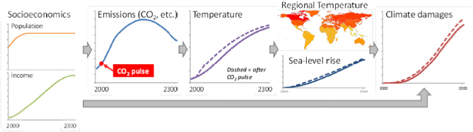
NOTE: Each figure in this chain represents a key element in the models used to produce estimates of the SCC with projections from one element flowing into the next element.
Population and income projections are inputs to the derivation of projections for both emissions and climate damages.
SOURCE: Developed from Rose et al. (2014). Reprinted with permission.
___________________
9Damages from global climate change include, but are not limited to, changes in net agricultural productivity, energy use, human health effects, and property damages from increased flood risk.
Each model takes as inputs a projection of human population growth and of global or regional income, as well as emissions paths of global greenhouse gases.10 A simple climate model component of each SCC-IAM translates the reference emissions trajectory into a reference global mean temperature trajectory and a reference trajectory of global mean sea level rise. In two of the models, regional average temperature trajectories are also derived from global mean temperature. Each model then uses one or multiple damage functions to translate temperature and sea level rise into economic damages or benefits. In the IWG analysis, global damages in the Climate Framework for Uncertainty, Negotiation and Distribution (FUND) and Policy Analysis of the Greenhouse Effect (PAGE) are an equally weighted sum of regional damages (i.e., no equity weighting) (Interagency Working Group on the Social Cost of Carbon, 2010, p. 11).
In order to derive an SCC estimate, the impact of a CO2 emissions pulse is calculated following the same causal chain: the CO2 pulse is introduced in a particular year, creating a trajectory of temperature (global and regional), sea level rise, and climate damages. The difference between this damage trajectory (the dotted line in Figure 2-1, above) and the reference trajectory (the solid line) in each year is discounted to the present using annual discounting (a constant annual discount rate in the IWG application). The resulting value is an SCC estimate for the given set of assumptions used in the reference and perturbed scenarios.
There are several steps in the causal chain for each SCC-IAM that are worth highlighting because they are different across models and have notable implications for the ultimate calculation of an SCC estimate. We discuss these differences in more detail below, but flag them here:
- emissions can vary in terms of their coverage and time path;
- the reference and perturbed temperature trajectories depend on the way the climate system is modeled within each SCC-IAM; and
- there are significant observed differences in the global climate responses across SCC-IAMs and the regional temperatures derived by downscaling (i.e., by establishing geographically fine-scale information from changes in aggregate climate conditions).
Chapter 4 explores the relevant aspects of the climate systems of the SCC-IAMs in greater technical detail.
Another aspect in which the SCC-IAMs differ is in the handling of damages. The models differ in the spatial and sectoral resolution of damages, and they differ in which sectors are the most important sources of climate damages. For two of the models (Dynamic Integrated Climate-Economy Model [DICE], and PAGE), damages are functions of only temperature and income, while for the other (FUND) they are also functions of the rate of temperature increase, CO2 concentrations, per capita income, population, and other drivers.
Overall, each SCC-IAM follows roughly the same causal chain in terms of the sequence of modeling information flow, yet differs in the model translations at each step. The IWG uses the following versions of three IAMs (IWG 2013, 2015):
___________________
10As designed, each of the three SCC-IAMs derives emissions from socioeconomic projections. However, in the IWG application of those models, socioeconomic and emissions projections were taken from an external source for two of the models, while the third derived its own fossil fuel combustion and industry CO2 emissions.
- the 2010 version of DICE by William Nordhaus;
- version 3.8 of FUND by Richard Tol and David Anthoff; and
- the 2009 version of PAGE model by Chris Hope.
We note, however, that the IWG model version may be different from the modeler’s original or most recent versions.
As mentioned above, the three models differ in the details of their implementation. Table 2-1 provides a broad summary of their dimensions. For a more comprehensive comparison of those differences, see Rose et al. (2014). Specific differences in socioeconomic and emissions modeling are described below, and, in Chapter 4, we discuss climate system modeling.
TABLE 2-1 SCC-IAM Coarse Feature Comparison
| DICE 2010 | FUND v3.8 | PAGE 09 | |
|---|---|---|---|
| Regions | 1 region | 16 regions | 8 regions |
| Damage Sectors | 2 sectors | 14 sectors | 4 sectors |
| Regional Temperature Downscaling | No | Yes | Yes |
| Damage Drivers | Temperature (level), income (total) | Temperature (level and growth), CO2 concentration, income (total and per capita), population size/composition, othera | Temperature (level), income (total and per capita) |
| Sea Level Rise (SLR) Damage Specification | Quadratic function of global sea level rise (i.e., Damage = αSLR2) |
Additive functions for coastal protection costs, dryland loss, and wetland loss, based on an internal cost-benefit rule for optimal adaptation | Power function of global sea level rise (i.e., Damage = αSLR0.7) |
| Damage Specification (Excluding Sea Level Rise) | Quadratic function of global temperature (i.e., Damage = αT2) |
Uniquely formulated by sector | Power function of regional temperature (i.e., Damage = αT1.76) |
| Model-Specific Parametric Uncertainties | None | Yes (in climate and damage modeling) | Yes (in climate and damage modeling) |
| “Catastrophic” or “Discontinuity” Damages Included | Yes (as expected damages) | No | Yes (as uncertain threshold) |
a“Other” includes: dryland value, wetland value, topography (elevation, coast length), protection cost, ocean temperature, and technological change.
SOURCE: Developed from Rose et al. (2014). Reprinted with permission.
As can be seen in the table above, there are several high-level structural differences among the SCC-IAMs. DICE is global (i.e., has only 1 region), while FUND and PAGE split the world into 16 and 8 regions, respectively. Each SCC-IAM covers multiple damage sectors, but only FUND disaggregates economic sectors in any detail. Since DICE is a global model, only FUND and PAGE downscale regional temperatures (with different methods).
The models also differ in the specific drivers of climate damages and their functional specification. DICE and PAGE use power functions—a quadratic or other polynomial function of temperature or sea level rise—for each of the represented sectors. FUND, on the other hand, disaggregates damage functions into a more detailed set of sectors. In addition, FUND and PAGE both consider model-specific climate and damage parametric uncertainty—each of those models allows for certain parameters to be drawn from probability distributions. Thus, FUND and PAGE reflect some uncertainty in their specifications; however, those characterizations and their implications vary between the two models (see Rose et al., 2014).
METHODOLOGY
The IWG methodology for constructing the official U.S. SCC estimates is discussed in detail in the IWG technical support documents (Interagency Working Group on the Social Cost of Carbon, 2010, 2013, 2015). The methodology results in 150,000 estimates of the SCC for each year and discount rate, yielding a frequency distribution of SCC results; see Figure 2-2. Percentiles and summary statistics of these estimates, also shown in Figure 2-2, are presented in the IWG technical support documents.11
In order to arrive at the 150,000 estimates for each discount rate, each of the three models was run 10,000 times with random draws from the equilibrium climate sensitivity (ECS) probability distribution (and other model-specific uncertain parameters), for each of the five socioeconomic scenarios (150,000 estimates = three models × five socioeconomic scenarios × 10,000 runs), for each of three discount rates (2.5 percent, 3 percent, and 5 percent).12 Frequency distributions of results for 2020 estimates were summarized for each model, socioeconomic scenario, and discount rate.
To facilitate the use of the SCC in regulatory analysis, the values of the SCC are averaged across the three SCC-IAMs and the five emissions scenarios, implicitly defining a frequency distribution of SCC values conditional on each discount rate. In averaging the results across models and emissions scenarios, all models and all emissions scenarios are given equal weight. Figure 2-2 is an example of the resulting frequency distribution for 2020 SCC estimates as reported in the IWG’s 2015 technical support documents.13 The average value of the SCC is shown for each discount rate, using a vertical line, as is the 95th percentile of the frequency distribution of SCC results for the case of a 3 percent discount rate. The larger SCC estimates in Figure 2-2 arise, in part, from realizations in the positively skewed right tail of the ECS distribution used by the IWG.
___________________
11The full set of estimates is available on request from the IWG.
12In terms of standardized uncertainties across all three models, five reference socioeconomic and emissions scenarios projected until 2300 were used, as well as one common probability distribution for the ECS parameter—the equilibrium temperature change that results from a doubling of CO2 relative to preindustrial levels. For FUND and PAGE, the IWG methodology included model-specific parametric uncertainties for both the climate and damage components.
13Summary statistics of the distribution of results for each model, conditional on discount rate and socioeconomic scenario are reported in an appendix of the IWG’s technical support document (Interagency Working Group on the Social Cost of Carbon, 2010, Appendix).
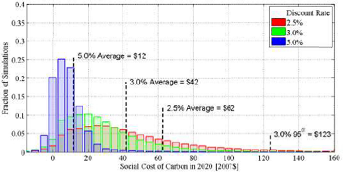
NOTES: Each histogram (red, green, blue) represents model estimates, conditional on one of three discount rates, over five different socioeconomic-emissions scenarios, 10,000 random parameter draws, and the three SCC-IAMs (see text for discussion). The frequency distributions shown represent most of the 150,000 SCC estimates. However, they do not represent the entire distribution. Some estimates fall outside the range of the horizontal axis shown.
SOURCE: IWG Technical Support Document (Interagency Working Group on the Social Cost of Carbon, 2015, Figure 1).
In the appendix to each technical support document, the frequency distribution of results based on 10,000 runs is summarized for the year 2020 for each SCC-IAM, emissions scenario, and discount rate. Specifically, the average value of the SCC is reported, as well as the 1st, 5th, 10th, 25th, 50th, 75th, 90th, 95th, and 99th percentiles of the frequency distribution of SCC estimates. Table 2-2 illustrates this for a discount rate of 3 percent for each emissions scenario (i.e., 15 sets of results).
TABLE 2-2 2020 Global SCC Estimates at a 3 Percent Discount Rate (2007 dollars/metric ton CO2).
| Percentile | 1st | 5th | 10th | 25th | 50th | Ave | 75th | 90th | 95th | 99th |
|---|---|---|---|---|---|---|---|---|---|---|
| Scenario | PAGE | |||||||||
| IMAGE | 4 | 7 | 9 | 17 | 36 | 87 | 91 | 228 | 369 | 696 |
| MERGE Optimistic | 2 | 4 | 6 | 10 | 22 | 54 | 55 | 136 | 222 | 461 |
| MESSAGE | 3 | 5 | 7 | 13 | 28 | 72 | 71 | 188 | 316 | 614 |
| MiniCAM Base | 3 | 5 | 7 | 13 | 29 | 70 | 72 | 177 | 288 | 597 |
| 5th Scenario | 1 | 3 | 4 | 7 | 16 | 55 | 46 | 130 | 252 | 632 |
| Scenario | DICE | |||||||||
| IMAGE | 16 | 21 | 24 | 32 | 43 | 48 | 60 | 79 | 90 | 102 |
| MERGE Optimistic | 10 | 13 | 15 | 19 | 25 | 28 | 35 | 44 | 50 | 58 |
| MESSAGE | 14 | 18 | 20 | 26 | 35 | 40 | 49 | 64 | 73 | 83 |
| MiniCAM Base | 13 | 17 | 20 | 26 | 35 | 39 | 49 | 65 | 73 | 85 |
| 5th Scenario | 12 | 15 | 17 | 22 | 30 | 34 | 43 | 58 | 67 | 79 |
| Scenario | FUND | |||||||||
| IMAGE | -13 | -4 | 0 | 8 | 18 | 23 | 33 | 51 | 65 | 99 |
| MERGE Optimistic | -7 | -1 | 2 | 8 | 17 | 21 | 29 | 45 | 57 | 95 |
| MESSAGE | -14 | -6 | -2 | 5 | 14 | 18 | 26 | 41 | 52 | 82 |
| MiniCAM Base | -7 | -1 | 3 | 9 | 19 | 23 | 33 | 50 | 63 | 101 |
| 5th Scenario | -22 | -11 | -6 | 1 | 8 | 11 | 18 | 31 | 40 | 62 |
SOURCE: IWG Technical Support Document (Interagency Working Group on the Social Cost of Carbon, 2015, Table A.3).
The official SCC estimates are reproduced in Table 2-3 below. For the given years of a CO2 emission (2010, 2015, 2020, etc.), the four estimates are the average SCC values conditional on the three discount rates, plus the 95th percentile of SCC estimates using a 3 percent discount rate. As noted in the IWG technical support document 2015 update (p. 2):
Three values are based on the average SCC from three integrated assessment models [SCC-IAMs], at discount rates of 2.5, 3, and 5 percent. The fourth value, which represents the 95th percentile SCC estimate across all three models at a 3 percent discount rate, is included to represent higher-than-expected impacts from temperature change further out in the tails of the SCC distribution.
SCC ESTIMATES
In summary, each single estimate of the 150,000 SCC estimates for each discount rate depends on the SCC-IAM used, the socioeconomic and emissions scenario, a draw from the assumed distribution of the ECS, and, for FUND and PAGE, a draw from the distributions of their particular uncertain parameters. The resulting four official SCC estimates for an emissions year are the mean of the 150,000 results for each discount rate, as well as the 95th percentile for the 3 percent discount rate (see Table 2-3).
TABLE 2-3 Revised Social Cost of CO2, 2010 - 2050 (in 2007 dollars per metric ton of CO2).
| Discount Rate Year |
5.0% Avg |
3.0% Avg |
2.5% Avg |
3.0% 95th |
|---|---|---|---|---|
| 2010 | 10 | 31 | 50 | 86 |
| 2015 | 11 | 36 | 56 | 105 |
| 2020 | 12 | 42 | 62 | 123 |
| 2025 | 14 | 46 | 68 | 138 |
| 2030 | 16 | 50 | 73 | 152 |
| 2035 | 18 | 55 | 78 | 168 |
| 2040 | 21 | 60 | 84 | 183 |
| 2045 | 23 | 64 | 89 | 197 |
| 2050 | 26 | 69 | 95 | 212 |
SOURCE: IWG Technical Support Document (Interagency Working Group on the Social Cost of Carbon, 2015, Table 2).
The most recent update of the official SCC estimates is shown in Table 2-3. SCC estimates are provided for different future years on the basis of modeling CO2 pulses applied in each decade (half decade values are interpolations). The SCC estimates rise over time because, in the models, future emissions produce larger incremental damages as the economy grows and temperature rises.
This page intentionally left blank.


