1

Physical Structure of the Existing
Grid and Current Trends

INTRODUCTION

Electricity is the lifeblood of modern society, and for the vast majority of people that electricity is obtained from large, interconnected power grids. Engineered to offer the ultimate in plug-and-play convenience, the wall outlet is actually the gateway to one of the world’s largest and most complex machines. Starting in the early 1880s with Thomas Edison’s Holborn Viaduct system in London and the Pearl Street Station in New York, serving a total of just 59 customers in lower Manhattan,¹ central station power rapidly developed so that within a decade electricity was ubiquitous in many cities around the world. In the decades that followed, high-voltage, interconnected power grids developed and many rural areas were electrified as well.

While the grid was initially fueled to a large extent by hydro (and still is in some countries such as Canada), in the United States coal was king, and the 20th century was powered by fossil fuels with up to 20 percent nuclear. Economies of scale resulted in most electric energy being supplied by large power plants. Control of the electric grid was centralized through exclusive franchises given to utilities, which in turn had an obligation to serve all existing and future customers. This relatively stable arrangement allowed numerous technical challenges to be overcome, resulting in the creation of the modern electric grid. Named by the National Academy of Engineering as the greatest achievement of the 20th century,² electrification has truly changed the world.

However, the grid that was developed in the 20th century, and the incremental improvements made since then, including its underlying analytic foundations, is no longer adequate to completely meet the needs of the 21st century. The next-generation electric grid must be more flexible and resilient. While fossil fuels will have their place for decades to come, the grid of the future will need to accommodate a wider mix of more intermittent generating sources such as wind and distributed solar photovoltaics. Some customers want more flexibility to choose their electricity supplier or even generate some of their own electricity, in addition to which a digital society requires much higher reliability. The availability of real-time data from automated distribution networks, smart metering systems, and phasor measurement units (PMUs) holds out the promise of more precise tailoring of the performance of the grid, but only to the extent that such large-scale data can be effectively utilized. Also, the electric grid is

___________________

¹ Con Edison, “A Brief History of Con Edison,” http://www.coned.com/history/electricity.asp, accessed February 19, 2016.

² National Academy of Engineering, “Greatest Achievements of the 20th Century,” http://www.greatachievements.org/, accessed February 19, 2016.

increasingly coupled to other infrastructures, including natural gas, water, transportation, and communication. In short, the greatest achievement of the 20th century needs to be reengineered to meet the needs of the 21st century.

Achieving this grid of the future will require effort on several fronts. Certainly there is a need for continued shorter-term engineering research and development, building on the existing analytic foundations for the grid. But there is also a need for more fundamental research to expand these analytic foundations. The purpose of this report is to provide guidance on the longer-term critical areas for research in mathematical and computational sciences that is needed for the next-generation grid. This chapter and Chapters 2 and 3 set the stage by providing a brief overview for the physical structure of the existing grid and some of the analyses that are essential for planning, evaluating, and operating the grid. Given the complexity of the existing grid, this introduction can only touch on some of the major topics and is certainly not comprehensive. More information is available in power systems textbooks such as Glover et al. (2012), Wood et al. (2013), Kundur (1994), or Van Cutsem and Vournas (2007).

BASIC GRID CONCEPTS

Interconnected Alternating Current Power Grids

While Edison’s original power grid was direct current (dc), it soon became apparent that power having low dc voltages (about 100 V) could be distributed over only a few blocks. This is because power is equal to the product of the voltage and current, and with 19th century technology there was no practical way of changing dc voltages. Hence higher currents were required, and since the transmission losses are proportional to the square of the current times the line resistance, power could not be efficiently transmitted over long distances. The alternative, alternating current (ac) power, championed by Nikola Tesla and George Westinghouse, soon won out because the voltage could be easily changed by devices known as transformers (though lower Manhattan remained fully dc until 1928, with the last dc service remaining until 2007³). So by the 1890s, ac transmission lines operating at tens of kilovolts (kV) were transmitting electricity dozens of miles, such as from a hydro power plant at Niagara Falls to Buffalo. Twenty years later electricity was transmitted hundreds of miles at voltages of about 100 kV, reaching 735 kV in the 1960s. Today the highest ac voltage used in North America is 765 kV, while a 1,000-kV grid is being developed in China, and countries in the former USSR have operated lines up to 1,150 kV (Huang et al., 2009).

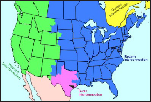
Excepting islands and some isolated systems, North America is powered by the four interconnections shown in Figure 1.1. Each operates at close to 60 Hz but runs asynchronously with the others. This means that electric energy cannot be directly transmitted between them. It can be transferred between the interconnects by using ac-dc-ac conversion, in which the ac power is first rectified to dc and then inverted back to 60 Hz.

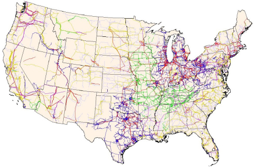
Any electric power system has three major components: the generator that creates the electricity, the load that consumes it, and the wires that move the electricity from the generation to the load. The wires are usually subdivided into two parts: the high-voltage transmission system and the lower-voltage distribution system. A ballpark dividing line between the two is 100 kV. In North America just a handful of voltages are used for transmission (765, 500, 345, 230, 161, 138, and 115 kV). Figure 1.2 shows the U.S. transmission grid. Other countries often use different transmission voltages, such as 400 kV, with the highest commercial voltage transmitted over a 1,000-kV grid in China.

The transmission system is usually networked, so that any particular node in this system (known as a “bus”) will have at least two incident lines. The advantage of a networked system is that loss of any single line would not result in a power outage. In some regions, a 69- or 46-kV subtransmission system, which may be networked, is also used.

The lower-voltage distribution system is usually radial, meaning there is just a single supply; networked distribution is sometimes used in urban areas. Typical distribution system voltage levels include 34.5, 13.8, 12.4, 4.16, and 2.4 kV. Distribution lines are often called feeders. Additional transformers step the voltage down to the load supply voltages of usually less than 1 kV (commonly 480 V for commercial and 120/240 V for residential customers).

___________________

³ J. Lee, “Off Goes the Power Current Started by Thomas Edison,” New York Times blog, March 4, 2011, http://cityroom.blogs.nytimes.com/2007/11/14/off-goes-the-power-current-started-by-thomas-edison/?_r=0.

While ac transmission is widely used, the reactance⁴ and susceptance⁵ of the 50-or 60-Hz lines without compensation or other remediation limit their ability to transfer power long distances overhead (e.g., no farther than 400 miles) and even shorter distances in underground/undersea cables (no farther than 15 miles). The alternative is to use high-voltage dc (HVDC), which eliminates the reactance and susceptance. Operating at up to several hundred kilovolts in cables and up to 800 kV overhead, HVDC can transmit power more than 1,000 miles. One disadvantage of HVDC is the cost associated with the converters to rectify the ac to dc and then invert the dc back to ac. Also, there are challenges in integrating HVDC into the existing ac grid.

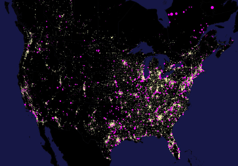
Commercial generator voltages are usually relatively low, ranging from perhaps 600 V for a wind turbine to 25 kV for a thermal power plant. Most of these generators are then connected to the high-voltage transmission system through step-up transformers. The high transmission voltages allow power to be transmitted hundreds of miles with low losses—total transmission system losses are perhaps 3 percent in the Eastern Interconnection and 5 percent in the Western Interconnection. With the advent of distributed photovoltaics, more generation is being directly connected to the distribution system, sometimes with supply voltages as low as 120/240 V for residential connections. Figure 1.3 shows the general distribution of load (white) and generation (magenta) in North America. Notice that in the East the load is more evenly distributed, with the generation closer to the load (except in Northeast Canada); in the West, much of the load is on the coast, with the generation spread throughout the interconnect.

Large-scale interconnects have two significant advantages. The first is reliability. By interconnecting hundreds or thousands of large generators in a network of high-voltage transmission lines, the failure of a single generator or transmission line is usually inconsequential. The second is economic. By being part of an interconnected grid, electric utilities can take advantage of variations in the electric load levels and differing generation costs to buy and sell electricity across the interconnect (a topic that is more fully discussed in Chapter 2). This provides incentive to operate the transmission grid so as to maximize the amount of electric power that can be transmitted. However, large interconnects also have the undesirable side effect that problems in one part of the grid can rapidly propagate across a wide region, resulting in the potential for large-scale blackouts such as occurred in the Eastern Interconnection on August 14, 2003. Hence there is a need to optimally plan and operate what amounts to a giant electric circuit so as to maximize the benefits while minimizing the risks.

Power Grid Time Scales

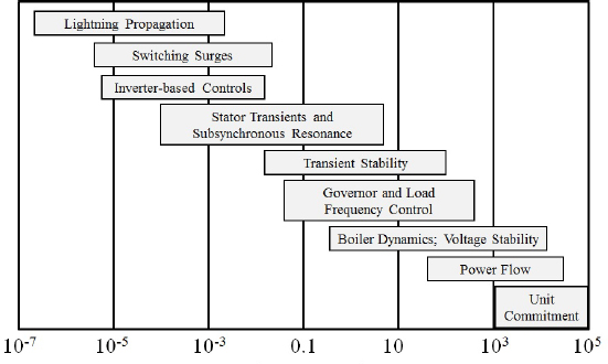
Anyone considering the study of electric power systems needs to be aware of the wide range in time scales associated with grid modeling and the ramification of this range on the associated techniques for models and analyses. Figure 1.4 presents some of these time scales, with longer term planning extending the figure to the right, out to many years. To quote University of Wisconsin statistician George Box, “Essentially, all models are wrong, but some are useful. However, the approximate nature of the model must always be borne in mind” (Box and Draper, 1987, p. 424). Using a model that is useful for one time scale for another time scale might be either needless overkill or downright erroneous.

As an example, a key aspect of power system design is what is known as insulation coordination—designing the grid to adequately protect power system equipment from the transient overvoltages caused by lightning strikes and switching surges. This requires dynamic models of the system response using time steps on the order of microseconds. Since voltages and currents propagate down the transmission lines at velocities near the speed of light (186,000 miles per second or 300 m/µsec), it is important to model the delays that occur as these waves propagate down the lines. Thus on a microsecond time scale the response of the grid becomes decoupled since what occurs at one location on the grid does not instantaneously affect more distant locations, allowing for the use of distributed simulation, a technique that makes simultaneous use of multiple arithmetic processors to reduce the time required to complete the simulation. This is quite different from the coupled algebraic equations that will be introduced in the next sections to model the transmission system in the slower time frames.

___________________

⁴ Reactance is the opposition of a circuit element to a change in current or voltage.

⁵ Susceptance is the reciprocal of reactance.

Basic Circuits—Quasi-Steady-State Time Frame

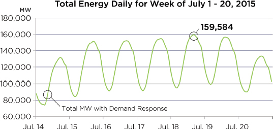
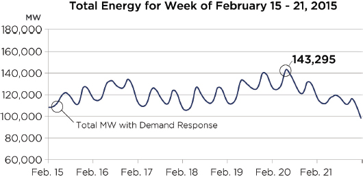
A good place to start the development of power system models is in what is known as the power flow time frame, or quasi-steady state. This is the time frame that would be perceived if one were to go into a utility control center in the common situation when there are no disturbances on the grid. Being an ac system, the voltages and currents would actually be varying at close to 60 Hz. But the displayed average power consumed by the load

would not show this variation. Rather, it would be slowly changing as it goes through its broader daily, weekly, and seasonal variation. Figure 1.5 shows an example of the weekly variation in the total aggregate electric load for PJM (a regional transmission organization in the Eastern Interconnection) during the summer, whereas Figure 1.6 shows an example of the same variation in winter. Likewise, the average generation dispatch would be slowly changing to match the variation in the electric load. So, even though the load might change by close to 100 percent in a single day, the change is slow—to the casual observer the grid would appear to be in near steady state.

To develop the models consider a sinusoidal voltage v(t) or current at a constant frequency, f (say, 60 Hz), so that

where Vmax is the maximum voltage level, ω = 2πf, and θV is a phase angle offset. The root mean square (rms) for this constant frequency sinusoidal is

If one were to model a network of voltage sources, current sources, resistors, inductors, and capacitors in which all the voltage and current sources were sinusoidal with the same frequency, then all the voltages and currents in the system would be sinusoidal at this frequency. The steady-state response of this uniform frequency network could then be modeled using phasor analysis in which

1. Each voltage and current is represented by a complex phasor value with the magnitude equal to its rms value and the angle equal to its phase angle.
2. Each resistance R is represented by an impedance Z_R = R.
3. Each inductance L is represented by an impedance Z_L = jωL.⁶
4. Each capacitance C is represented by an impedance Z_C = 1/(jωC).
5. The relationship between the phasor voltage and current in a device with impedance Z is given by Ohm’s law, V = ZI; admittance is defined as the inverse of impedance, so Y = 1/Z.

The instantaneous power consumed in a device with a sinusoidal voltage v(t) across the device and sinusoidal current i(t) into the device is

which can be rewritten by applying trigonometric identities as a nonzero average power and a component with double the original frequency:

in which V is the rms voltage, I the rms current, and P the average power over a period. Since the average value of the second (sinusoidal) component over a period is zero, for the quasi-steady-state time frame only the average power is of interest. The complex power can be defined as

where the magnitude of S is known as the apparent power, P as the real power, and Q as the reactive power. Real power is usually expressed in megawatts (MW), reactive power in megavars (Mvar), and apparent power in megavoltamperes (MVA). The physical significance of the reactive power is difficult to describe. Reactive power is defined mathematically in (5). Its physical significance is difficult to describe, but roughly speaking, reactive

___________________

⁶ Where j is defined as the imaginary unit using electrical engineering notation to avoid confusion with the symbol i used for current.

power represents energy stored for part of an electrical cycle in the magnetic field and released later in the cycle. It is required in order to make many electrical devices, such as the induction motors used in air conditioners and refrigerators, function correctly. The concept of reactive power is quite useful for power system analysis and it is treated in a manner analogous to the real power. It is easy to show that resistors always consume real power, inductors always consume reactive power, and capacitors always generate reactive power.

Three-Phase Power Systems and Per-Phase Analysis

High-voltage power systems are almost always three phase. In a three-phase system there are three conductors instead of the two conductors found in dc circuits or single-phase circuits. A three-phase system is considered balanced if the voltages and currents (respectively) have equal magnitude but are shifted in phase from each other by 120°. The phases are usually labeled A, B, and C. Two key advantages of balanced three-phase systems (compared to single-phase) are (1) for the same amount of wire twice the power can be transferred and (2) three-phase electric devices such as generators and motors are more efficient and hence more economical than single-phase devices with the same power rating.

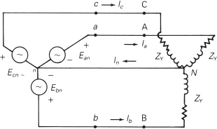
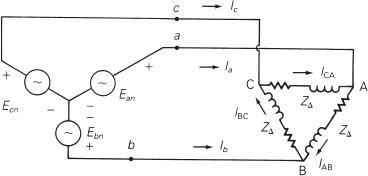
Three-phase systems can either be Y-connected (wye-connected) or Δ-connected (delta-connected). Figure 1.7 shows an example of a Y-connected voltage source on the left supplying a Y-connected load on the right; in a balanced three-phase system, the neutral current, In, would be zero, so this conductor could be omitted. In a balanced three-phase system the line-to-line voltages (e.g., Ea-Eb in the figure) are square root of 3 greater than the line-to-neutral voltages (e.g., Ean). Since nominal transmission line voltages are expressed in line-to-line values, a 345 kV transmission line would have line-to-neutral values of 200 kV. Figure 1.8 shows a Y-connected voltage source and a Δ-connected load. Both wye and delta connections are commonly used in the power grid.

The actual power grid is never perfectly balanced. Most generators and some of the load are three-phase systems and can be fairly well represented using a balanced three-phase model. While most of the distribution system is three-phase, some of it is single phase, including essentially all of the residential load. While distribution system designers try to balance the number of houses on each phase, the results are never perfect since individual household electricity consumption varies. In addition, while essentially all transmission lines are three phase, there is often some phase imbalance since the inductance and capacitance between the phases are not identical. Still, the amount of phase imbalance in the high-voltage grid is usually less than 5 percent, so a balanced three-phase model is a commonly used approximation.

In order to model the interconnected power network, appropriate models need to be developed for the transmission lines, transformers, generators, and loads. The analysis of a balanced three-phase system can be greatly simplified by using a technique known as per-phase analysis, in which the system is treated as an equivalent single-phase system.

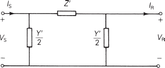
In the steady-state time frame a reasonable per-phase model for a transmission line is what is known as the π-equivalent circuit, consisting of a series impedance Z′ between two shunt admittances Y′/2 (Figure 1.9). The maximum amount of power that can be transferred through a transmission line, sometimes due to thermal constraints, is often represented as the maximum power in megavolt amperes, or MVA limit.

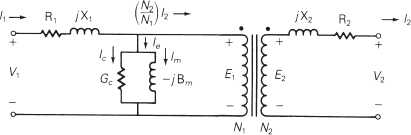
Likewise, a reasonable steady-state transformers model consists of a series impedance and shunt admittance, except now in series with an ideal transformer model (shown in Figure 1.10). In an ideal transformer model, the ratio of the voltages, E1/E2, is identical to the turns ratio of the windings, at = N1/N2, and the ratio of the current into the E1 side versus the current out of the E2 side is the inverse of the turns ratio. The maximum amount of power that can be transferred through a transformer is also often represented as an MVA limit.

In order to easily analyze networks with transformers it is helpful to introduce what is known as per-unit (PU) analysis, in which the system values are normalized using base values that depend on a systemwide power base and voltage bases that differ by the turns ratios of the ideal transformers. PU analysis can be used with either single-phase systems or, as presented here, three-phase systems. For three-phase PU, first select a single three-phase base power for the entire system, Sb,3ϕ; 100 MVA is typical. Then select line-to-line voltage bases that differ by the ideal transformer turns ratios, Vb,LL; these values are typically the nominal transmission voltages (e.g., 500, 345, 138 kV). Current, impedance, and admittance bases can then be defined as

All network complex powers, voltages, currents, and impedances are converted to PU by normalizing by their corresponding base values, which are quantities in the nominal steady-state operating conditions. PU values are still complex numbers but are dimensionless. When using PU, the ideal transformers are eliminated from the

transformer models. This results in a model of the network consisting of just PU impedances and admittances, greatly simplifying the network analysis. By using a three-phase PU base, a balanced three-phase system can be solved as though it were a single-phase system. With proper accounting of the 30° phase shift in transformer voltages for the wye-delta connection, the analysis is the same whether a device is connected as wye or as delta.

To study an interconnected system the relationship between the PU phasor voltages and bus (node), current injections can be obtained by applying Kirchhoff’s current law (KCL) at each bus in the system. That is, the equality constraints are obtained by recognizing that the net current being injected into each bus must be equal to the current flowing out of the bus into the rest of the network. Using matrix notation for a network with N buses gives

where Y is the N×N bus admittance matrix, I is an N-dimensional column vector of the net phasor current injections at each bus, and V is the N-dimensional column vector of the bus voltages. In a large network, Y will be quite sparse since there is only a nonzero off-diagonal entry Ykn if there is a direct connection between buses k and n.

If the generator outputs could be represented as complex current injections and the loads as shunt admittances, then this equation could be used to determine V, and by using V with the branch models (with “branch” used generically to refer to the transmission lines and transformers), all the system complex powers could be determined. Unfortunately, the generator outputs cannot be represented as current injections, and the loads are not well modeled as shunt admittances. Rather, to determine V the nonlinear power flow equations need to be formulated and solved.

ILLUSTRATIVE TYPES OF ANALYSIS NEEDED FOR THE GRID

Power Flow—Steady-State Analysis

The power flow or load flow (the two terms have been used interchangeably since at least the 1960s) is the most widely used power system analysis technique either as a stand-alone application or embedded in other applications. The goal of the power flow is to determine the quasi-steady-state V vector, given a specified set of generation and load values. To develop the power flow equations, it is necessary to first present time-scale-appropriate generator and load models.

On the power flow time scale, generators are usually most appropriately modeled as a constant real power injection (P) into the system at a specified per unit (PU) bus voltage magnitude (V). Hence the generator is assumed to be modifying its reactive power output (Q) to keep its terminal (bus) voltage magnitude constant. This is known as a PV bus. Loads are often represented as constant negative real power (P) and reactive power (Q) injections into the system and are known as PQ buses. However, because in the quasi-steady-state time frame the total real power generation must exactly match the total real-power-load bus losses, the outputs of all the generators cannot be independently specified. Rather, at least one generator is designated as the slack (or swing) bus, in which the voltage magnitude and angle at the generator’s bus is specified, and the power flow algorithm determines the generator’s real and reactive power output.

Power flow equation derivation starts with applying KCL at each bus so that the net current injection into the bus must equal the current going into the network. And since the complex power is the voltage times the conjugate of the current, the net complex power injection into the bus must equal the complex current into the network. For bus k, the relationships are

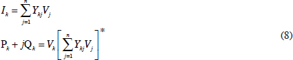
where Pk and Qk are the specified real and reactive power injections at bus k. Expressing the complex numbers with the following notation,

these complex equations are typically written as the real-valued power balance equations

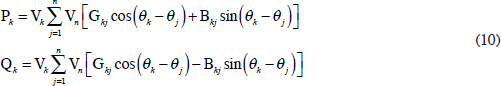
Hence the power flow problem is the solution of a set of 2n nonlinear algebraic equations given by (10). For PV buses the reactive power balance equations are not included since the voltage magnitude at these buses is specified; the reactive power outputs of the PV generators are dependent variables. For the slack bus, neither equation is included since both the real and reactive power output of the generators are dependent variables.

Power flow models can come in all different sizes, from just a few buses for academic systems, to a representation of an entire interconnect. When modeling a large system it is certainly not possible nor is it needed to represent each individual load. Rather, since the distribution system is usually radial it is often sufficient in power flow studies to represent all the devices on a distribution feeder as a single, aggregate load. In addition, equivalent models can be developed that further reduce the number of buses that need to be represented. Currently the Eastern Interconnection, with a total load of about 650 GW, is modeled with about 65,000 buses, while 20,000 buses are currently used for the Western Interconnection, with a total load of about 170 GW.

Figure 1.11 shows an example power flow solution for a small seven-bus system. The results are shown on a “oneline diagram” (oneline) in which the actual three-phase transmission lines are represented by a single line. As is common for engineering studies, voltages are reported in PU, so assuming a 138-kV voltage base, the actual line-to-line voltage magnitude shown in the figure in yellow at bus 1 as 1.05 PU would be 1.05 × 138 kV = 144.9 kV. The oneline shows the real and reactive power outputs for all the generators (shown as black circles), the aggregate

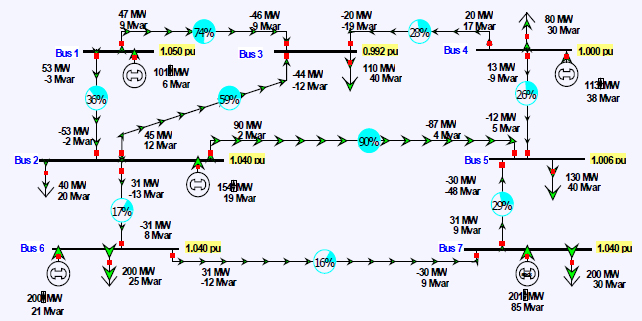
bus loads (shown as black arrows), and the transmission lines. Note that both the real and reactive powers at each bus sum to zero, with a sign convention that power into each transmission line at the bus is assumed positive. The green arrows show the flow direction of the real power. Because of line resistance the amount of real power out of a line is always less than the power into it. With reactive power this is not always the case since the transmission line model includes capacitance terms (which create reactive power). The PU bus voltage magnitudes are shown with the yellow fields. Buses 1, 2, 4, and 6 are modeled as PVs with a fixed voltage magnitude, and bus 7 is the system slack. The pie charts show the percentage loading for each of the transmission lines, with the limit for each line specified in terms of either maximum MVA or maximum amps. Oftentimes these limits are due to thermal considerations, recognizing that as the lines’ conductors heat up they expand, resulting in increased sag for overhead conductors.

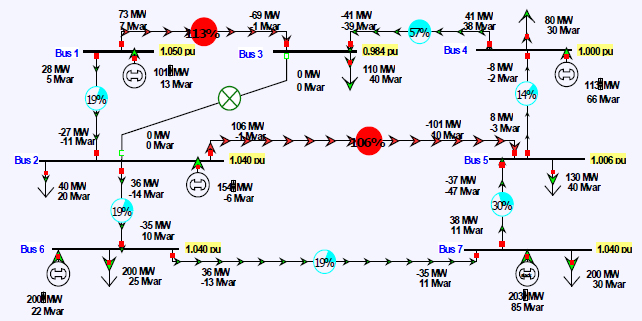
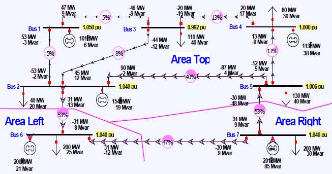
The power flow is commonly used to determine how modifications to the generation, load, or system topology would affect the flows throughout the system. Figure 1.12 shows the previous example, except now with the transmission line between bus 2 and bus 3 out. If this outage had occurred on an actual system there surely would have been transient changes to the system (as per Figure 1.4), including switching surges, and transient stability oscillations. But assuming the system remained stable, within several seconds it would have settled back to the quasi-steady-state power flow solution shown in Figure 1.12. Except for the topology change, all the power flow inputs (i.e., the load real and reactive values, and the generator real power and voltage setpoint values) remained constant. The only changes were to the power-flow-dependent variables, including the PQ bus voltage magnitudes, the PV generator reactive power outputs, and the slack bus real and reactive outputs. A single contingency, such as opening the line between buses 2 and 3, also changes the flows throughout the system, albeit with the largest changes usually closest to the contingency.

This example also illustrates that the transmission line flows are dependent variables—they cannot be directly controlled. In general, they can only be indirectly controlled, such as by changing the generator real power outputs (exceptions are phase-shifting transformers and HVDC transmission lines that do allow direct flow control). This is illustrated in Figure 1.13, where the transmission line overloads from the previous contingency are removed by reducing the real power output of generator 6 from 200 to 101 MW. Note a corresponding increase in the bus 7 (slack) generation, from 203 to 300 MW; the net change in the two generators does not sum exactly to zero

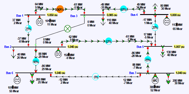
because of a slight change in the real power losses. In addition to branch limits, reliable power system operation also requires that the bus voltage magnitudes be within a reasonable range, usually between about 0.95 and 1.05 PU.

When modeling large-scale power systems, the basic power flow algorithm presented here is augmented to model the response of various continuous and discrete power system controllers. While the details are beyond the scope of this brief introduction, examples include load-tap-changing (LTC) transformers, phase-shifting transformers, switched capacitor banks, automatic generation control, HVDC transmission lines, and more advanced generator voltage control. Hence the power flow is solving a set of nonlinear algebraic equations,

where g is a vector of algebraic constraints including the real and reactive power balance equations, y is the solution variable vector such as the PQ bus voltage magnitudes and angles, and u is the input parameter vector such as the load real and reactive power values. Both y and u might contain a mixture of continuous and discrete values.

One common approach to avoid solving the nonlinear equations of (11), used particularly with the market analysis discussed in Chapter 2, is to assume the approximations shown in (12). First, since the resistances of the transmission lines are often much less than their reactances, the conductance terms are assumed to be zero. Second, since the voltage magnitudes are usually close to 1.0 PU, they are assumed to be just that. Third, given that the angle differences across the lines are small, the cosine terms are assumed to be unity and the sine terms are approximated as the angle differences. Last, the reactive power constraints are ignored. This reduces the power flow to a set of linear equations,

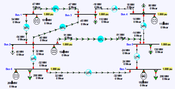
with the inputs P and B used to solve for θ. This approximation is known as the dc power flow, with the nonlinear power flow often referred to as the ac power flow. Note that both are still ultimately providing solutions to an ac circuit, with the dc power flow just a linear approximation. The validity of the approximations is quite system specific. To illustrate, Figure 1.14 contains the dc power flow solution for the seven-bus system whose ac power flow solution is given in Figure 1.12.

Interconnected Power System Steady-State Operations

The basics of steady-state operations can be fairly well thought of as a slowly changing power flow solution. As the load slowly varies, the values of various controls are changed, either automatically or manually by the power system operator, and the line flows respond to them. The most crucial control is the modification of the real power outputs of the generators to match changes in the system load, a process known as automatic generation control (AGC).

While an interconnected grid is just one big electric circuit, many of them, including the North American Eastern and Western Interconnections, were once divided into “groups”; at first, each group corresponded to an electric utility. These groups are now known as load-balancing areas (or just “areas”). The transmission lines that join two areas are known as tie lines, and the algebraic sum of the real power flow on the tie lines for an area is known as its net interchange, with the usual sign convention that power flow out of an area is defined as positive.

The area control error (ACE) for area k is then defined as

where NI_A,k is the actual net interchange in MW, NI_S,k is the scheduled net interchange in MW, β_k is an area-specific bias term in MW/0.1 Hz (with a negative sign), F_A is the actual system frequency in hertz, F_S is the scheduled system frequency in hertz, and I_ME,k is the interchange metering error term that is usually small or zero (NERC, 2011). The scheduled system frequency is usually 60 Hz, but it can be either 59.98 or 60.02 Hz for time error correction. The ACE for each area and the system frequency are the most important numbers associated with the system’s operation; ACE is kept close to zero by using AGC to adjust the generation to match the changing load.

With this approach it is possible to easily implement power transactions between different areas. These are known as bilateral transactions, since they involve two players. The scheduled net interchange for each area is just equal to the sum of its transactions. Modifying the scheduled net interchange causes a change in the ACE, causing AGC to adjust the outputs of generators in the area. This is demonstrated in Figure 1.15, in which the original system is now subdivided into three areas: top (containing buses 1 to 5), left (containing bus 6), and right (containing bus 7). The system is modeled with a single 100-MW transaction going from right (the seller) to left (the buyer). The system is modeled with the ACE for each area equal to zero, so the net flow across each area’s

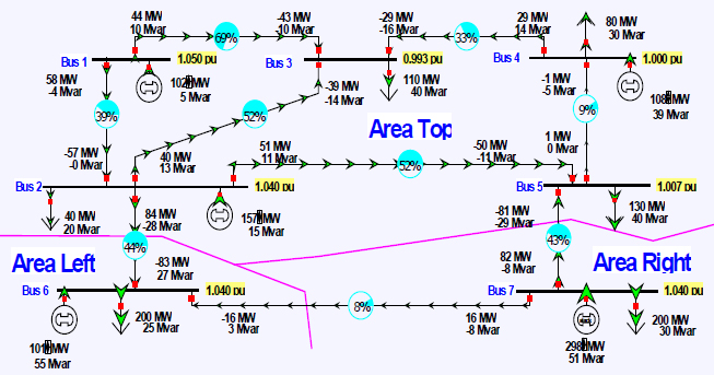
tie lines is equal to its schedule values (with the power flow assumption that the actual and scheduled frequencies are 60 Hz). When the flows in Figure 1.15 are compared to those in the original Figure 1.11, it is seen that a single transaction can impact the flows across an interconnect.

Power transactions between different players (e.g., electric utilities, independent generators) in an interconnection can take from minutes to decades. In a large system such as the Eastern Interconnection, thousands of transactions can be taking place simultaneously, with many of them involving transaction distances of hundreds of miles, each potentially impacting the flows on a large number of transmission lines. This impact is known as loop flow, in that power transactions do not flow along a particular “contract path” but rather can loop through the entire grid.

With a power flow solution, the incremental impact of each transaction can be calculated from sensitivity analysis, with the sensitivities of how much a single transaction impacts the flows on each line known as power transfer distribution factors (PTDFs). The PTDFs for the Figure 1.15 transaction are visualized in Figure 1.16, with the pie charts and arrows now showing the percentage of the right to left transaction that flows on each line, with a total of 100 percent leaving the right and arriving at the left.

Because the electric grid is regularly subject to faults and other disturbances (e.g., lightning hitting a transmission line or a generator failing), a crucial aspect of power system operations is the need to continue operating with no limit violations even when subject to such contingencies. Examples of limits include keeping the transmission line and transformer flows below a specified MVA value and keeping the bus voltage magnitudes within a PU range (e.g., between 0.95 and 1.05 PU). The standard operating paradigm is to be at least N − 1 reliable, meaning that if any single credible contingency were to occur there would be no limit violations. N − 1 reliability is assessed using contingency analysis (CA), which in its simplest form consists of running potentially thousands of power flow solutions, each considering a different contingency. Online CA is commonly run in electric control centers on about a 5-minute interval. Since each contingency is independent, CA may be easily parallelized.

Another common online analysis tool is optimal power flow (OPF). The purpose of OPF is to minimize some scalar value, such as total operating cost, while satisfying various equality and inequality constraints:

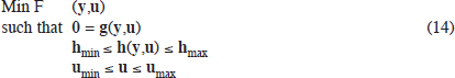
The key equality constraints are the power balance equations from the power flow shown in equations (11), while the key inequality constraints are the need to operate with the branch flows, bus voltage magnitudes, and generator reactive powers within their limits. The system controls may be either continuous (e.g., generator real power outputs) or discrete (e.g., transformer tap positions, switched shunt status). Figure 1.17 shows an example of an OPF solution for the seven-bus case. The one line has been modified to show the incremental cost of enforcing the real power constraint at each bus (in $/MWh), a value known as the locational marginal cost (LMP); LMPs are widely used in the operation of electric power markets (discussed in the next chapter). Also, as is common in actual power markets, a color contour is used to visualize the variation in the LMPs. In this example the system is segmented because of the MVA limit on the line between buses 2 and 5. OPF is commonly combined with CA to determine the optimal dispatch taking into account all the contingencies, so the final solution is N − 1 reliable (something that was not done in Figure 1.17). This is known as security-constrained optimal power flow, (SCOPF). As originally formulated, the OPF used the full ac power flow equations as given in (10). This is now often refereed to as the ACOPF. A new, more approximate approach uses the dc power flow equations given in (12). This is often referred to as the DCOPF. Likewise, the SCOPF can be formulated using either the ac power flow equations or the dc equations. Commonly, however, the terms OPF and SCOPF are used generically to refer to either the ac or the dc approach.

In order to run the previous analysis techniques online with an actual grid, it is first necessary to obtain a starting power flow solution that matches as closely as possible the actual grid conditions. This is done in a process known as state estimation (SE), in which a large number of imperfect measurements, such as bus voltage magnitudes and line-flow real and reactive flow values, are used to obtain the solution of equations (11) that best matches the measurements. Electric control centers typically run SE every few minutes. In contrast to power flow

in which the number of variables matches the number of equations, SE is an overdetermined problem. A discussion of the currently used algorithms for solving power flow—CA, OPF, and SE—is contained in Chapter 4.

Day-Ahead Planning and Unit Commitment

In order to operate in the steady state, a power system must have sufficient generation available to at least match the total load plus losses. Furthermore, to satisfy the N − 1 reliability requirement, there must also be sufficient generation reserves so that even if the largest generator in the system were unexpectedly lost, total available generation would still be greater than the load plus losses. However, because the power system load is varying, with strong daily, weekly, and seasonal cycles, except under the highest load conditions there is usually much more generation capacity potentially available than required to meet the load. To save money, unneeded generators are turned off.

The process of determining which generators to turn on is known as unit commitment. How quickly generators can be turned on depends on their technology. Some, such as solar PV and wind, would be used provided the sun is shining or the wind blowing, and these are usually operated at their available power output. Hydro and some gas turbines can be available within minutes. Others, such as large coal, combined-cycle, or nuclear plants, can take many hours to start up or shut down and can have large start-up and shutdown costs.

Unit commitment seeks to schedule the generators to minimize the total operating costs over a period of hours to days, using as inputs the forecasted future electric load and the costs associated with operating the generators. As will be considered in Chapter 2, unit commitment constraints are a key reason why there are day-ahead electricity markets. Complications include uncertainly associated with forecasting the electric load, coupled increasingly with uncertainty associated with the availability of renewable electric energy sources such as wind and solar.

The percentage of energy actually provided by a generator relative to the amount it could supply if it were operated continuously at its rated capacity is known as its capacity factor. Capacity factors, which are usually reported monthly or annually, can vary widely, both for individual generators and for different generation technologies. Approximate annual capacity factors are 90 percent for nuclear, 60 percent for coal, 48 percent for natural gas combined cycle, 38 percent for hydro, 33 percent for wind, and 27 percent for solar PV (EIA, 2015). For some technologies, such as wind and solar, there can be substantial variations in monthly capacity factors as well.

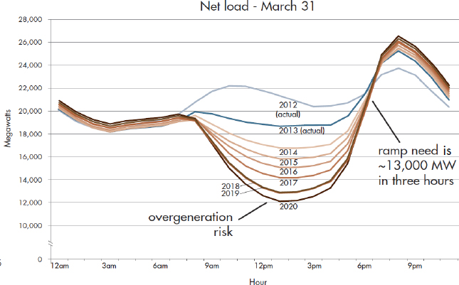
One issue associated with day-ahead planning is the need to ensure there is sufficient generation that can change (ramp) its output quickly in order to meet changes in the net load. As illustrated in Figure 1.5, ramping of generation to meet the changing load has long been a part of power system operations. However, with the growth in solar PV generation, ramping is becoming more of an issue as the net load rapidly decreases in the morning as the sun rises and falls in the evening as it sets. This impact of solar PV is illustrated in Figure 1.18, in what is known in the industry as the “duck” curve, because it resembles the aquatic bird.

Longer-Term Power System Planning

Much of the preceding discussion applies both to online operations and planning. However, planning has some unique aspects that deserve special consideration. Planning takes place on time scales ranging from perhaps hours in a control room setting, to more than a decade in the case of high-voltage transmission additions. The germane characteristic of the planning process is uncertainty. While the future is always uncertain, recent changes in the grid have made it even more so. Planning was simpler in the days when load growth was fairly predictable and vertically integrated utilities owned and operated their own generation, transmission, and distribution. Transmission and power plant additions could be coordinated with generation additions since both were controlled by the same utility.

As a result of the open transmission access that occurred in the 1990s, there needed to be a functional separation of transmission and generation, although there are still some vertically integrated utilities. Rather than being able to unilaterally plan new generation, a generation queue process is required in which requests for generation interconnections needed to be handled in a nondiscriminatory fashion. The large percentage of generation in the queue that will never actually get built adds uncertainty, since in order to determine the incremental impact of each new generator, an existing generation portfolio needs to be assumed. They cannot be considered independently. There

is also the question of who bears the risk associated with the construction of new generation. More recently, additional uncertainty is the growth in renewable generation such as wind and solar PV and in demand-responsive load.

Power System Stability

Switching attention to the faster time scales, transient stability is concerned with power system behavior on time frames ranging from about 0.01 sec to perhaps a few dozen seconds. In contrast to power flow, which seeks to determine a quasi-steady-state equilibrium point (EP), transient stability seeks to determine whether following a system contingency, such as a short circuit or loss of a generator, the system will return to an equilibrium point that may, however, often be different from the original EP. The general form of the problem is as a set of differential algebraic equations (DAEs):

in which x is a vector of state variables, u is the vector of system inputs, and y is the vector of algebraic variables, with many entries similar to the power flow variables such as the bus voltage magnitudes and angles. The starting point for a transient stability study is usually a power flow, and the initial values for x are determined by solving f(x,y,u) = 0.

Many of the differential equations contained in f are associated with modeling the behavior of the synchronous machines during this time frame. The most important of the synchronous generator differential equations is what is known as the generator swing equation, which can be expressed for generator k as two first-order differential equations,

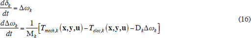
where δk and Δωk are state variables (elements of x) that represent the generator’s rotor torque angle and the generator’s deviation from synchronous speed; T_mech,k is the mechanical torque input to the generator; T_elec,k is the electrical torque output from the generator; D_k is a damping coefficient; and M_k is a value that depends on the inertia of the electric generator. The generator swing equation is commonly written in terms of mechanical and electric power rather than torque, with the rationale that the machine’s speed is usually quite close to synchronous speed.

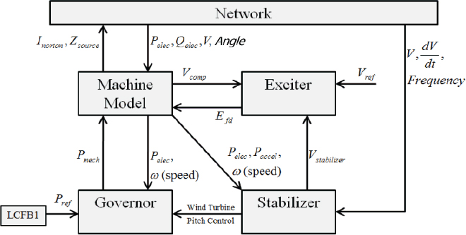
Commonly generators are represented with additional differential equations for the electric machines, for their exciters (to control the terminal voltage), for their governors (to control the mechanical power input), and for their stabilizers (to reduce system oscillations). A block diagram of these relationships is shown in Figure 1.19, with often a dozen or more differential equations modeled per generator. Load dynamics, such as those of induction motors, can also be included.

For a large system a single transient stability solution might involve the integration of more than 100,000 differential equations with tens of thousands of algebraic constraints using a time step of perhaps ¼ cycle (0.004166 sec for 60 Hz). Traditionally, transient stability solutions involved just a few seconds of simulation looking at “first swing” instability, though now they can run for dozens of seconds, looking at the longer-term behavior of quantities such as frequency and bus voltage magnitudes.

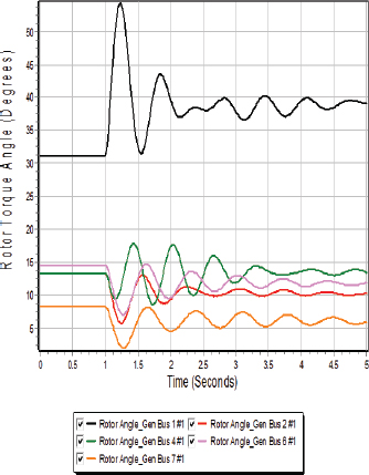
Figure 1.20 shows an example of first swing stability, plotting the generator torque angles for the seven-bus system shown in Figure 1.11, which has been augmented to include generator dynamic models. In this example the contingency is a low impedance fault at 1.0 sec near bus 1 on the transmission line between buses 1 and 2, which is cleared after three cycles (0.05 sec) by opening this line. During the fault the voltage at bus 1 is quite depressed, which greatly reduces the power output from generator 1, causing the generator to accelerate, increasing its torque angle with respect to the other generators. When the fault is cleared, the voltage is increased, with the simulation indicating that the system returns to a new quasi-steady-state equilibrium point.

In addition to generator torque angles, quantities of interest during a transient stability study include the generator speeds, the bus voltage magnitudes, and the bus frequencies. As a large case example, Figure 1.21 shows the generator speeds for an 18,000-bus case with a contingency modeling the opening of two large generators.

There has recently been increased interest in power system dynamics on the transient stability time frame. This is partially due to growing concerns about blackouts caused by transient stability issues, but also to greatly increased deployment of synchronized PMUs. By taking advantage of accurate time measurements available thanks to the Global Positioning System, PMUs can determine the power system voltages and current magnitudes and angles at typically 30 times per second. This is in contrast to the existing Supervisory Control and Data Acquisition systems, which return measurements every 4 to 12 seconds. Hence, transient stability time frame dynamics can now easily be viewed in real time at control centers, allowing for greatly improved modeling and analysis capabilities, and there is a growing desire to run transient stability studies in an online environment. Such an application would start from the SE solution (or even one directly observed by the PMUs) and then sequentially solve potentially thousands of contingencies. However, like traditional CA, this transient stability CA would be naturally parallelizable, since the transient stability for each contingency could be considered separately.

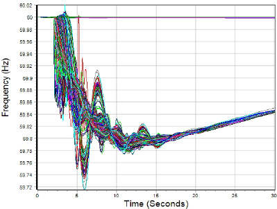
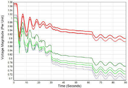
Situated between the power flow and transient stability time frames is voltage stability, defined as “the ability of a power system to maintain steady voltages at all buses in the system after being subjected to a disturbance from a given initial operating condition” (Kundur et al., 2004). The term “voltage collapse” is often used when voltage stability is lost, resulting in an uncontrolled decline in system voltages. According to a joint IEEE/CIGRE task force, voltage stability can be classified two ways—by the size of the disturbance and by the duration of the disturbance (Kundur et al., 2004). With respect to disturbance size, large-disturbance voltage stability considers the time domain response of a system after a large disturbance such as a generator outage, while small-disturbance voltage stability considers system response to small perturbations about a particular operating point. With respect to time, short-term voltage stability considers time frames on the order of several seconds, while long-term voltage stability extends the analysis to potentially many minutes. Transient stability analysis, augmented with appropriate additional models such as generator overexcitation limiters and LTC transformer dynamics, can be used to assess many aspects of voltage stability. Figure 1.22 shows an example of a short-term voltage collapse scenario, using the 18,000-bus case and contingency from Figure 1.21, augmented with some additional contingencies. The thick red lines show the decline in the PU voltage magnitude at several 500-kV buses, the green lines three 230-kV buses, and the blue lines three 115-kV buses.

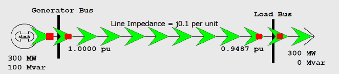
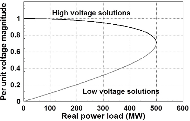
Usually power flow analysis is used to determine the risk to long-term, small-disturbance voltage stability by gradually increasing the system load (or some other parameter set) until the power flow equations no longer have a solution. This analysis is known as PV and/or QV analysis, since the bus voltage magnitudes are typically plotted with respect to either the real power (P) or the reactive power (Q) variation. An example of the PV curve for the two-bus case shown in Figure 1.23 is given in Figure 1.24. Here, provided the load is less than 500 MW, the power flow equations have two solutions, with the higher-voltage solution corresponding to the system operating point. A bifurcation point occurs at 500 MW, where the two solutions coalesce. This is the point of maximum loadabilility and would correspond to the long-term, small-disturbance voltage stability limit; the algebraic power flow equations have no solution for higher values of P. Having adequate reactive power is crucial to avoiding voltage instability. Several sources for reactive power are synchronous generators, static var compensators, and switched shunt capacitor banks. While the reactive power provided by the capacitors helps to support the voltage, a capacitor’s reactive power output varies with the square of its voltage, meaning that as the voltage starts to fall its reactive power also rapidly decreases, resulting in a potential instability. Hence the reactive power supplied by the other devices can be crucial.

In referring back to Figure 1.4, the time scales of transient stability and voltage stability fall between the quasi-steady-state power flow and the faster switching surges, harmonics, and subsynchronous resonance. Like power flow, the assumption is that speed of light effects in the transmission network can be ignored, though this assumption is certainly less valid given that it can take 10 msec for light to transit a 2,000-mile grid, so the coupled algebraic power balance equations assumed in equation (15)(15) cannot be fully true with a 4.16-msec time step. Even though the power system frequency is varying, the assumption is that the variation is small relative to the nominal frequency, with the branch impedances assumed fixed. So the transmission system is actually modeled assuming a fixed frequency. The impact of higher-frequency harmonics (e.g., 120, 180, . . . Hz) are not considered. Also, subsynchronous resonance, which might occur at frequencies between 10 and 30 Hz, an area of growing concern with wind farm installations, cannot be considered. Some generator and control system dynamics are included in transient stability, but faster ones (such as generator stator transients) are ignored.

Faster power system phenomena are usually studied by setting up a full three-phase model of the grid and then representing the transmission lines with the differential equations associated with the voltage and current relationships in inductors and capacitors. By using trapezoidal integration techniques, the models reduce to a network of coupled current sources and shunt resistances in which transmission line propagation delays can be considered

explicitly. Integration time steps can then be as small as necessary to represent the phenomena of interest, such as 50 µsec for a switching transients study. An advantage of this approach is that a portion of a system can be solved in parallel since there is a natural decoupling due to the transmission line propagation delays. However, because of the small time constants, this approach requires large amounts of hardware for studies of even small systems.

Distribution Systems

As was mentioned earlier, the portion of the system that ultimately delivers electricity to most customers is known as the distribution system. This section provides a brief background on the distribution system as context for the rest of the report; further details are available in books such as Kersting (2012), Willis (2004), or Glover et al. (2012).

Sometimes the distribution system is directly connected to the transmission system, which operates at voltages above, say, 100 kV, and sometimes it is connected to a subtransmission system, operating at voltages of perhaps 69 or 46 kV. At the electrical substation, transformers are used to step down the voltage to the distribution level, with 12.47 kV being the most common in North America (Willis, 2004). These transformers vary greatly in size, from a few MWs in rural locations to more than 100 MW for a large urban substation.

The electricity leaves the substation on three-phase “primary trunk” feeders. While the distribution system can be networked, mostly it is radial. Hence on most feeders the flow of power has been one-way, from the substation to the customers. The number of feeders varies by substation size, from one to two up to more than a dozen. Feeder maximum power capacity can also vary widely from a few MVA to about 30 MVA. Industrial or large commercial customers may be served by dedicated feeders. In other cases smaller “laterals” branch off from the main feeder. Laterals may be either three phase or single phase (such as in rural locations). Most of the main feeders and laterals use overhead conductors on wooden poles, but in urban areas and some residential neighborhoods they are underground. At the customer location the voltage is further reduced by service transformers to the ultimate supply voltage (120/240 for residential customers). Service transformers can be either pole mounted, pad mounted on the ground, or in underground vaults. Typical sizes range from 5 to 5,000 kVA.

A key concern with the distribution system is maintaining adequate voltage levels to the customers. Because the voltage drop along a feeder varies with the power flow on the feeder, various control mechanisms are used. There include LTC transformers at the substation to change the supply voltage to all the substation feeders supplied by the transformer, voltage regulators that can be used to change the voltage for individual feeders (and sometimes even the individual phases), and switched capacitors to provide reactive power compensation.

Another key concern is protection against short circuits. For radial feeders, protection is simpler if the power is always flowing to the customers. Simple protection can be provided by fuses, but a disadvantage of a fuse is that a crew must be called in the event of it tripping. More complex designs using circuit breakers and re-closers allow for remote control, helping to reduce outage times for many customers.

While distribution systems certainly require substantial initial design (Willis, 2004, provides a good overview of planning considerations), the distribution system has traditionally “been characterized as the most unglamorous component” of an electric power system (Kersting, 2012). Most distribution systems are either unmetered or have customer meters that might be read only monthly, so that distribution systems are often overdesigned.

However, this is rapidly changing. With reduced costs for metering, communication, and control, the distribution system is rapidly being transformed. Distributed generation sources on the feeders, such as PV, mean that power flow may no longer be just one-way. Widely deployed advanced metering infrastructure systems are allowing near-real-time information about customer usage. Automated switching devices are now being widely deployed, allowing the distribution system to be dynamically reconfigured to reduce outage times for many customers. Advanced analytics are now being developed to utilize this information to help improve the distribution reliability and efficiency. Hence the distribution system is now an equal partner with the rest of the grid, with its challenges equally in need of the fundamental research in mathematical and computational sciences being considered in this report.

ORGANIZATION OF THE REPORT

Chapter 1, “Physical Structure of the Existing Grid and Current Trends,” Chapter 2, “Organizations and Markets in the Electric Power Industry,” and Chapter 3, “Existing Analytic Methods and Tools,” lay out the current structure of the power grid, the economic markets involved in ultra-short-term decision making to long-term planning, and the analytic techniques that are currently used to study the behavior of the grid. Chapter 4, “Background: Mathematical Research Areas Important for the Grid,” narrows the focus to the mathematics needed and currently used for these analyses.

Chapter 5, “Preparing for the Future,” discusses the sources of uncertainty inherent in predicting the structure of the future grid and some of the general mathematical tools that may be needed. Chapter 6, “Mathematical Research Priorities Arising from the Electric Grid,” examines research challenges for mathematics where progress will enable new technologies. Although a wide range of research areas have potential importance, this report will

not discuss all of them in detail. Rather, it concentrates on the two areas that the committee felt were most relevant to the grid: optimization and dynamical systems. Advances in these areas could have widespread impacts, regardless of how the overall grid evolves.

In Chapter 7, “Case Studies,” the report illustrates the diversity of mathematical problems, along with solutions, where they are now being solved. The problem of coordinating bid-based expenses with offer-based costs while satisfying regulatory, physical, operating, and business constraints—the unit commitment problem first described in Chapter 2—is given a representation as a mathematical programming problem. Other case studies illustrate the difficulty and importance of predicting low-frequency high-impact events, improving the resilience of the grid, and increasing the capability for handling anticipated massive amounts of data.

In Chapter 8, “Building a Multidisciplinary Research Community,” the committee presents recommendations that will enlarge the community of researchers to include power engineers, mathematicians, and, potentially, other scientists—for example, statisticians and economists.

REFERENCES

Box, G.E.P., and N.R. Draper. 1987. Empirical Model-Building and Response Surfaces. Wiley, New York, N.Y.
California ISO. 2013. “What the Duck Curve Tells Us about Managing a Green Grid.” http://www.caiso.com/documents/flexibleresourceshelprenewables_fastfacts.pdf.
EIA (U.S. Energy Information Administration). 2015. Electric Power Monthly. July. Washington, D.C.
Glover, J.D., M.S. Sarma, and T.J. Overbye. 2012. Power System Analysis and Design, 5th ed. Cengage Learning, Boston, Mass.
Huang, D., Y. Shu, J. Ruan, and Y. Hu. 2009. Ultra high voltage transmission in China: Developments, current status and future prospects. Proceedings of the IEEE 97(3):555-583.
Kersting, W.H. 2012. Distribution System Modeling and Analysis, 3rd ed. CRC Press, Boca Raton, Fla.
Kundur, P. 1994. Power System Stability and Control. McGraw-Hill Education, New York, N.Y.
Kundur, P., J. Paserba, V. Ajjarapu, G. Andersson, A. Bose, C. Canizares, and N. Hatziargyriou. 2004. Definitions and classification of power system stability. IEEE Transactions on Power Systems 19(3):1387-1401.
NERC (North American Electric Reliability Corporation). 2011. “Balancing and Frequency Control,” January 26. http://www.nerc.com/docs/oc/rs/NERC%20Balancing%20and%20Frequency%20Control%20040520111.pdf.
Pai, M.A., P.W. Sauer and Thomas J. Overbye. 2012. Data-driven power system operations. Pp. 448-455 in Computational Science—ICCS 2006 (V.N. Alexandrov, G.D. van Albada, and P.M.A. Sloot, eds.), Proceedings, Part III, Lecture Notes in Computer Science 3993. Springer-Verlag, Berlin, Heidelberg. Sauer, P.W., and M.A. Pai. 2007. Power System Dynamics and Stability. Stipes Publishing, Champaign, Ill. January 18.
Van Cutsem, T., and C. Vournas. 2007. Voltage Stability of Electric Power Systems. Springer, New York, N.Y.
Willis, H.L. 2004. Power Distribution Planning Reference Book, 2nd ed. CRC Press, Boca Raton, Fla.
Wood, A.J., B.F. Wollenberg, and G.B. Sheble. 2013. Power Generation, Operation and Control, 3rd ed. Wiley-Interscience, Hoboken, N.J.