3

Existing Analytic Methods and Tools

INTRODUCTION

Since the genesis of electric grids in the early 1880s the amount of expertise that has been gained in their operation and planning is enormous. And over the last 60 years, much of that expertise has been embedded in software that is of increasing complexity. In order to estimate the mathematical and computational research needed for the next-generation electric grid it will be important to first consider some of the existing analytic methods that are used in this already quite sophisticated software to plan and operate the grid of today. Building on the foundation described in Chapters 1 and 2, such consideration is the purpose of this chapter. Chapter 4 then covers the mathematical underpinnings for these algorithms.

An important caveat is that the algorithms presented here were developed to meet the needs of a grid that was initially operated by vertically integrated utilities that obtained most of their electricity from centrally controlled, large-scale generators. Scenarios for how the grid of the future might evolve are discussed in Chapter 5, with subsequent chapters discussing how the techniques presented here will need to evolve and research will need to move forward. Another important caveat: The committee focuses here on common algorithms that are widely used by the power industry. Given the wide-ranging scope of the literature in the field, it would be impossible to comment on all of the many approaches that have been proposed for solving the cited problems. And even with this caveat the chapter can only scratch the surface of power grid applications, providing brief coverage for some of the key algorithms, their underlying assumptions, and their approximations.

POWER FLOW (LOAD FLOW)

As was described in the first chapter, power flow is the key to solving quasi-steady-state power balance equations, allowing calculation of the per-unit voltage magnitude and angle at every bus (node) in the system. Usually the power flow also involves calculating the values for a host of continuous and discrete power system controllers as well, such as tap positions for load-tap-changing (LTC) transformers and the status of switched reactive control devices such as capacitors. Once all of these values have been determined, the power flowing on all of the system transmission lines and transformers (branches) can be determined. The power flow solution can then be used to check whether system quantities are within their limits (e.g., transmission line and transmission flows are less than the limits, and voltage magnitudes are between their minimum and maximum limits). Power flow is probably the most common power system analysis technique.

Historically the first power flows were done using analog computers, known as network analyzers. As digital computers started to become common in the 1950s and 1960s the use of network analyzers was replaced by numerical techniques. Since the power flow equations are nonlinear, their solution required an iterative approach. The Gauss-Seidel approach was initially the most common technique since its solution worked well on computers with limited memory, with 50-bus systems solved in the 1950s on computers with 2 kilobytes (kB) of memory (Brown and Tinney, 1957). However, convergence could be slow. While still taught and occasionally used, it has mostly been replaced by algorithms based on the Newton-Raphson (NR) approach.

Power flow solution by the NR method, or some variation of it, is currently the most common technique, having been introduced in 1967 (Tinney and Hart, 1967). The NR method takes advantage of the fact that each bus in a power system is joined to only a handful of other buses, making the network incidence matrix sparse and leading to a sparse Jacobian matrix. Taking advantage of the development of sparse matrix methods in the 1960s, including improved ordering algorithms pioneered to a large extent by power engineers (Sato and Tinney, 1963), the NR method could be applied to larger systems on computers with limited memory. In 1967 (Tinney and Hart, 1967) a 949-bus system was solved, with each iteration taking 10 seconds on an IBM 7040 and leading to speculation that a 2,000-bus network could be solved on a computer with 32 kB of memory. The quadratic convergence of Newton’s method allows solutions of even large systems in just a few iterations. However, Newton’s method-based algorithms can fail to converge for ill-conditioned problems, which can occur when the system voltage is outside a “normal” range. Improving the convergence of the power flow has been an area of active research for many years (Iwamoto and Tamura, 1981) and continues to require research. This is partially due to the fractal domains of attraction for power flow solutions (Demarco and Overbye, 1988; Thorp and Naqavi, 1989).

Over the years several enhancements were proposed, including the fast decoupled power flow (Stott and Alsac, 1974), which eliminated the need for updating the Jacobian inverse at every iteration, and the transformation of the Jacobian/network matrix to orthogonal eigenvectors, which has the potential for speedier solutions and improved iterations. The dc power flow model is also common, particularly in power market analysis, in which the nonlinear equations are approximated by a set of linear equations, eliminating the need for the iterative NR algorithm.¹

The largest power flow cases routinely solved now contain at most 100,000 buses.² While this is a significant increase from the hundreds of buses modeled 50 years ago, the size of the largest power flow problems (with on the order of a million nonzeros in the Jacobian) is now quite modest compared to both the growth in computer memory and problems in other domains, which may have billions of nonzeros. Interconnected system power flow models are not expected to grow in size significantly because the radial distribution system can be effectively aggregated for interconnect-wide studies.

There are actually two types of power flow models. The one that is most often used, and almost exclusively employed in large-scale system studies, assumes that the underlying three-phase system is balanced. This allows the use of per-phase models in which the actual three-phase system can be treated as though it were an equivalent single-phase system. This is also known as the positive sequence model. The second type, known as the three-phase power flow, explicitly models the three phases including their mutual couplings, allowing it to handle unbalanced conditions. Presently, the three-phase power flow is mostly used to model distribution systems or microgrids in which significance imbalance could occur, as well as detailed models of distribution circuits where some branches are only one or two phases. If the three-phase power flow were used on large system models, the number of buses would increase by a factor of three and the number of Jacobian elements by a factor of nine. However, getting and using the data needed to set up such models would be a challenge. The remainder of this section refers to the more common balanced, three-phase approach.

As a stand-alone application, the power flow is used in situations ranging from real-time studies in a control center to planning studies looking at system conditions decades in the future. For near-real-time studies the power flow case would be derived from the output of the real-time state estimator (discussed later), which combines

___________________

¹ As mentioned in Chapter 1, the dc power flow is a linearized solution method that is used to give solutions to the ac power flow; it has nothing to do with the solution of actual dc systems.

² The term case is used to refer to the power system model parameters needed to solve a power flow. At a minimum a case would include a list of the bus parameters (such as their numbers, names, nominal kilovolts), generator and load parameters (including their net power injection values), and transmission line and transformer parameters.

models of the system components (such as the impedances of the transmission lines) with actual system data. In this situation it might be used to determine the impact of an anticipated control action on the real-time system. For longer-term planning studies (e.g., years to decades into the future) the power flow could be used to determine the consequences of proposed system changes, such as new transmission and generation, coupled with changes in the load.

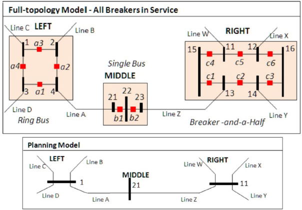
Historically there has been a difference between how the power system is represented in real-time power flows and the longer-term planning power flows. The real-time approach has used what is known as a “node-breaker” full-topology model in which the many actual power system switching devices (such as circuit breakers and disconnects) are represented, with their terminals designated as nodes. Since the switches have essentially zero impedance, when the power flow is solved these nodes are dynamically consolidated, through what is known as topology processing, into a much smaller number of buses. Each bus then corresponds to a set of nodes. So a 100,000-node system might be reduced to perhaps 20,000 buses. This is needed for real-time analysis in which detailed models of the substation topology are available and the status of the switches is known. In the planning context, in which this information is usually not available or may not be fully known for future substations, a more aggregated model is used in which most switches are not explicitly modeled (see Figure 3.1). This difference in modeling assumptions has resulted in a divide between software designed for real-time usage and that for planning applications. However, newer planning software is increasingly able to bridge this divide by directly supporting the node-breaker models.

There are several sources of uncertainty in power flow cases. Usually the reactance and susceptance terms used in the models of the branches are known with good accuracy. There is, however, some uncertainty associated with the resistance term because the resistivity of aluminum and copper has a temperature sensitivity of 0.4 percent per degree Celsius and the actual conductor temperature is seldom known. (The conductor temperature varies in some locations by more than 100°C over the course of a year.) Usually the system solution is relatively insensitive to

resistance errors since the reactances of the high-voltage lines can be many times their resistive values. As resistance heating changes the effective length of the conductor due to thermal expansion effects, the inductance also changes slightly owing to changed geometry. Understanding line-sag effects in real time is a crucial operational issue as excessive sag can lead to conductor-to-tree faults.

The uncertainty in the assumed load and generation depends on the application. In real time these values are provided from the state estimator and would have little error. In day-ahead and longer studies the load uncertainty would depend on the accuracy of the forecast. In longer-term studies there is also uncertainty surrounding which generation and transmission resources would actually be available. The voltage magnitude dependence of the load can also be a source of uncertainty since it ultimately depends on the actual composition of the load, which is continually varying—for example, air-conditioning usage through the course of a summer day or patterns of use for lighting through the day. For an uncontrolled resistive load (such as incandescent lighting) the power varies with the square of the voltage, whereas for electronics there is often essentially no voltage dependence (unless the voltage gets too low). Almost always a constant load power model is assumed.

Another issue with power flow algorithms is assumptions on the response of the embedded power system controls to a change in the system state. These assumptions can cause different software packages to have potentially quite different results; yet each result is valid in that it satisfies all of the specified solution criteria. For example, opening a transmission line would cause a change in the bus voltage magnitudes. A number of continuous and discrete control devices would respond to changes in the bus voltages, including generator reactive power outputs, static var compensators, transformer LTC taps, and automatically switched shunts. For an actual system, how these devices would respond and how they are coordinated depends on their dynamics, as well as on the actions a human operator might take, such as manually changing switched capacitors to keep generator reactive power outputs within the middle of their range to provide reactive reserves. While the basic power flow algorithm is rather simple, much of the sophistication of commercial software packages lies in their handling of these control responses.

The complete set of model parameters necessary to solve the power flow is referred to as a “case.” A power flow case would at least have parameters associated with the buses, the generators, the load, and the transmission lines and transformers. Different commercial power flow packages may support different numbers of parameters for the different object types. For example, some packages allow the specification of the latitude and longitude for the buses, and they allow buses to be grouped into substations, while others do not. Cases can represent either entirely fictitious (synthetic) power systems—for example, the seven-bus case from Chapters 1 and 2—or an actual power system.

Within North America, power flow cases are available for all four major interconnects. Until 2001 some of these cases were publicly available through the U.S. Federal Energy Regulatory Commission’s FERC715 filings. Subsequent to an October 11, 2001, FERC order, these power flow cases have been treated as confidential for national security reasons, but interested persons may submit a Critical Energy Infrastructure Information request to obtain access. Power flow cases can also sometimes be obtained for research purposes through nondisclosure agreements with electric utilities.

The cases can be interchanged between different software packages using several text file formats, with the formats changing slightly from software version to version. One current impediment to research is that some of the power flow text file formats used in the exchange of power flow data, such as with the FERC715 filings, are proprietary and not fully available to the public. While many researchers in the power discipline have access to these formats since they have purchased the commercial software, this would be less true for researchers in other disciplines such as mathematics. The Institute of Electrical and Electronics Engineers (IEEE) did publish a public format in 1973 (Working Group on a Common Format for Exchange of Solved Load Flow Data, 1973), but it was never updated and is now essentially obsolete. The text file formats permitted for the FERC cases are listed in FERC (2010). Another impediment to research is that there are few publicly available large-scale cases. Since security concerns limit the distribution of actual system cases, an alternative would be the creation of synthetic cases with characteristics like those of the actual system. But even the distribution of synthetic data is limited unless the formats used for their exchange are publicly available—this issue is further discussed in Chapter 8.

Recommendation 2: The Federal Energy Regulatory Commission (FERC) should require that all text file formats used for the exchange of FERC715 power flow cases be fully publicly available.

While power flow analysis is widely used, there are certainly still open research issues. The first is power flow convergence. Being nonlinear, the power flow equations can have multiple solutions or even no solution. Whether a solution is found and, if it is, whether it is the desired solution depends on the initial guess. Commercial practice for large systems is to start a new power flow from the previous solution; few commercial software packages can actually reliably determine a solution if they are not provided with a reasonable initial guess, usually a previous solution. Determining if the desired solution has been found is also a challenge. Complicating convergence is the presence of many additional system automatic controls that must be considered, including discrete controls with either narrow regulation ranges that might not allow for a solution, or wide ranges that allow for a range of solutions. The use of proprietary or specific control algorithms for particular apparatus, as opposed to generic models, creates issues when exchanging cases between different software packages. The increased penetration of inverter-based resources creates needs for rapid development of accurate models and controls and incorporation of these into public models as well as codes. High-voltage dc transmission links, static-var compensators, and now wind farm and solar interconnection are among the many examples of inverter-based resources. As four-quadrant inverters capable of volt/var support become required, this question becomes more and more important. Inverters also cause novel problems in dynamic analyses and harmonic analyses, as discussed below.

A second research issue is dealing with the stochastic nature of the loads and generation. Current practice is to assume a deterministic model, which can then be precisely solved (convergence issues aside). However, even a small amount of uncertainty in some of the loads or generation can result in an almost unmanageable potential range in solutions. This is becoming more of an issue, in particular because of the growth in stochastic renewable generation resources.

STEADY-STATE CONTINGENCY ANALYSIS

An important application of the power flow is known as steady-state contingency analysis (CA), where the adjective steady-state is used to distinguish it from the dynamic contingency analysis discussed later in this chapter in the section “Transient Stability and Longer-Term Dynamics.” As touched on in Chapter 1, reliable grid operation requires that the grid be able to operate even with the loss of any single device (e.g., a branch or a generator). This is known as N – 1 reliability. CA refers to the automated process of doing such calculations, in which a set of contingencies is first defined, with each contingency modifying the system in some way, such as the removal of one or more devices. CA then solves each contingency in the set, either sequentially or in parallel, to determine if there are any postcontingency violations.

The earliest automated CA procedures date to the early 1960s (El-Abiad and Stagg, 1963), in which the power flow was just sequentially solved for all the branches in the case. Over the next several decades a number of improvements were introduced, including the recognition that since most contingencies will not cause postcontingency violations they can be processed quite quickly by more approximate contingency screening methods. Since the impact of most contingencies is local, a common screening technique is to apply the contingency to a much smaller equivalent system. The much faster dc power flow algorithm is also used for linear screening. Matrix compensation methods such as the matrix inversion lemma can be used to avoid continually fully factoring the sparse matrix for the incremental changes caused by a single device outage. Bounding algorithms are also used to limit the extent of the solutions required by quickly determining that the final solution will not exceed limits based on initial iterative results.

Online CA has been used in control centers since the 1980s (Subramanian and Wilbur, 1983), running now as often as every minute. For a control center for a large area, many thousands of individual contingencies can be simulated. However, CA is a naturally parallel application because the solution of each contingency is independent of the solutions of the other contingencies. Accordingly, the solution times can be greatly reduced with the use of parallel processing. Sometimes screening techniques are used, and sometimes a full solution is done for each contingency.

As computer speeds have increased, the N – 1 criterion is giving way to what is known as N – 1 – 1. In this approach the initial N – 1 contingencies are solved. During this solution for each N - 1 contingency the postcontingent solution is adjusted using criteria to mimic the actions that would likely be taken immediately after the contingency has occurred (such as generation re-dispatch, phase shifter adjustment, voltage optimization, and load shifting). Then the entire N – 1 set is again applied to each of the originally N – 1 contingencies. Computationally this is of order N². The North American Electric Reliability Corporation (NERC) has standards for which contingencies need to be considered (NERC, 2015).

Another newer development is more detailed consideration of contingencies that are likely to initiate cascading failures. Such contingencies are those that would probably cause other devices to fail, resulting in a cascading sequence and, potentially, a large-scale blackout. This is known as N – k analysis, with newer algorithms having been developed to identify such situations.

The CA solution can also require special modeling of automatic actions that would quickly take place following a contingency. Such actions go by different names in different interconnections, including remedial action scheme (RAS), special protection system, and, sometimes, operating procedures. One such action might be to automatically trip a set of generators or lines immediately following a line outage, or to do automatic switching to transfer the supply for a load.

In designing a CA application, special attention must be paid to avoid the “data overwhelm” situation that would occur if a precontingent system already had existing violations. Without such attention, running thousands of contingencies would result in an unmanageable number of contingent violations. New statistical and uncertainty-analysis-based methods need to be developed to provide probabilistic or robust guarantees accounting for uncertainty and fluctuations in loads, renewables, and other components of the system. One issue with CA is that the probability of a given contingency occurring varies widely. Therefore risk-based CA needs to be investigated more thoroughly. NERC is developing criteria for risk-based CA, or stochastic CA, where cases to be studied would be weighted based on some assessment of their relative probability of occurrence and where N – 2 or N – k cases with multiple outages would come into play if the risk assessment so indicated. This is an important area for future research and should be incorporated into the ACOPF research from Recommendation 1.

CA has traditionally been a power flow (steady-state) based problem. Dynamic studies of outages were done manually using transient stability (TS) simulations (see below), which studied if the system could reach a new steady state without physical instability. But for large disturbances, especially ones that cause generators to shift their outputs, there is a growing trend to integrating CA with TS, in which rather than just being solved using power flow the contingencies are solving using TS. This allows determination of the longer-term dynamics (generation response) and whether the system remains secure as it moves to a new steady state.

OPTIMAL POWER FLOW AND SECURITY-CONSTRAINED OPTIMAL POWER FLOW

In its simplest form, the purpose of optimal power flow (OPF) is to optimize an objective function (usually energy costs, but—potentially—losses or other metrics) subject to security and operational limits on voltages and branch flows and subject to the overarching electrical equations as represented in the power flow model. The OPF has been a topic of research and development since the 1950s, when the first digital power flow algorithms were introduced for economic dispatch of the power grid. The problem becomes one of finding the best set of control variables (generation, voltage set points, and so on) such that when a set of these is selected for best objective function and the other injections (load) are input, the power flow solution will be feasible and no constraints violated. It was formulated in the 1960s using a Lagrangian function to minimize generation cost subject to the equality constraints from the power flow and the inequality constraints on both the controllers (e.g., the generator outputs) and other values such as the voltage magnitudes and transmission line flows (Dommel and Tinney, 1968).

Early research utilized the generalized reduced gradient approach, utilizing penalty functions to enforce the binding constraints. The advent of cheap and efficient linear programming (LP) solutions led to LP-based OPF algorithms, with compromises made in the representation of cost functions to accommodate LP formulations.

In the early 1970s the OPF was augmented to include not just constraints associated with violations in the base case power flow but also constraints that could arise because of CA violations (Alsac and Stott, 1974). This is

now known as the security-constrained OPF (SCOPF). The goal of the SCOPF is to determine the optimal control settings for the base system, such that the objective function is minimized while simultaneously ensuring there are no violations in the base case or in any of what could be a large number of contingency cases.

While easy to describe, the SCOPF can be quite difficult to fully solve. This is because it is a large-scale, nonlinear optimization that includes a mix of discrete and continuous controls wrapped around the power flow and CA problems. The problem is nonconvex and may admit multiple locally optimal solutions. Today no widely used commercial SCOPF algorithms include methodology to determine if multiple local solutions exist, and most algorithms rely on restrictive formulations to ensure adequate convexity. Additionally, stopping criteria in terms of the change in the objective function as well as changes in the solved state vector can be somewhat ad hoc. A distinction must also be made between the control actions that need to take place precontingency (i.e., need to be applied to the actual solution) and those that would only need to be taken postcontingency. Postcontingency actions, which would include the RASs discussed previously, would only need to occur in the unlikely event the contingency actually occurs. The presence of control algorithms within the solution can lead to discrete variables and discontinuities.

Today’s solution approaches take advantage of the several-orders-of-magnitude improvements that have taken place over the last two decades in mixed-integer LP algorithms and in nonlinear programing algorithms. As mentioned in Chapter 2, the SCOPF that is used for determining LMPs in most markets is based on the simplified dc SCOPF that utilizes a dc (as opposed to full ac) power flow model. Typical LMP comparisons between the ac and dc SCOPF methods are given in Overbye et al. (2004). Application of the full ac SCOPF therefore remains an open research issue, with a survey of current approaches covered in Castillo and O’Neill (2013) and more details given in Chapter 6. Future issues around the transmission–distribution interface may well arise if resources on the distribution system are to be included in the SCOPF solution of the transmission grid.

STATE ESTIMATION

In order to work in real time, power flow, CA, and SCOPF require a real-time model of the current system’s operating condition. This is provided by what is known as state estimation (SE). Originally formulated in 1970 by Schweppe and Wildes, SE combines a model of fixed system parameters such as the branch impedances, with actual system measurements of quantities such as circuit breaker statuses, bus voltage magnitudes, branch flows, and generator/load injections. The output is the estimated state variables (e.g., the voltage magnitudes and angles), which can then be used to determine the real-time power flow solution that best matches the system measurements. To function, SE requires that the number of measurements be greater than the number of estimated system states (i.e., the system needs to be overdetermined) and that all parts of the system be observable from the measurements.

As normally formulated, SE is a maximum likelihood estimator, where error statistics are assumed for the measurements but no a priori information is assumed about the state variables. The estimated states are those that maximize the likelihood of the set of observations used as inputs. The process is only modeled to the extent of the power flow equations—no process dynamics are modeled. Thus, as opposed to a Kalman filter, power system state estimation is a nonlinear static state estimation problem as formulated. SE is commonly solved using an iterative, weighted-least-squares approach.

If all the measurement errors are assumed to be uncorrelated, the problem is only slightly more difficult than the power flow problem. In the real world, measurements are correlated, so measurement bias is an issue (as opposed to having normally distributed zero mean error, as is commonly assumed). While research has been done on estimating measurement bias, the only enhanced application in use is “bad data detection,” where the statistics of the estimated residuals (i.e., the difference between the measured and estimated values) can be used to detect the presence of one or more “bad” data points and then successive estimates without those points are used to validate the bad data identification. This in turn can be used to detect the presence of measurement error, which would also affect basic Supervisory Control and Data Acquisition operation. It is also possible in theory, and as demonstrated in research projects, to use state estimation results over time to estimate network parameters. Practically speaking, this is not widely used because considerable manual intervention is required to pick the parameters to estimate. There are also research-level algorithms to detect and correct topology errors that are due to incorrect switch

and breaker status information. However, to date these algorithms have not been widely deployed commercially. These can be formulated to be performed on a substation basis without the need for solution of the ac network equations—Kirchhoff’s current law and logic are sufficient.

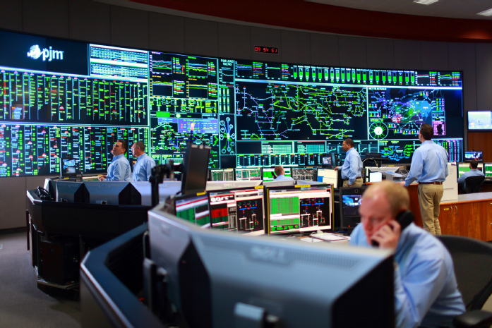
In the control room, shown in Figure 3.2, the online model provided by the SE is the input to all the other advanced tools (power flow, CA, SCOPF). The best-developed control room state estimators can solve large networks with on the order of 250,000 measurements every minute. However, if for some reason the SE solution does not converge, then an up-to-date model would not be available for these tools. Currently the best large-scale SEs converge well over 98 percent of the time (PJM, 2015). However, convergence alone may not be a sufficient test of the validity of the input assumptions on measurement accuracy and the solution. Rather, a chi-squared test of the measurement residuals (Schweppe and Masiello, 1971) should be applied to see if the solution is “reasonable” given the assumed error statistics.

The deployment of phasor measurement units (synchrophasors, or just PMUs, discussed in Chapter 1), which measure the system voltages and currents (both magnitudes and phase angles) at about 30 times per second, has allowed the development of “direct” state estimation, meaning that explicit, direct noniterative solutions of the power flow equations using phase angles (as measured) as inputs are possible; this is also known as a linear SE. These solutions can be performed very rapidly, at data acquisition scan rates of 10 seconds or less, to provide calculated network conditions as though they were measured. PMU data can also be used to directly estimate the parameters of a branch between two PMU measurement points (in conjunction with measured branch flows)—something that is useful in detecting potential transmission line sag as a function of line loading and ambient conditions.

The use of SE on the distribution system is not a well-developed methodology, nor is it in widespread use as typically there are not sufficient redundant measurements to warrant its application.

Including control algorithms for locally autonomous apparatus (as with the power flow problem) is not a well-developed methodology in SE either, and the advent of more and more inverter-based resources capable of local volt/var control will likely make this a more important question.

TRANSIENT STABILITY AND LONGER-TERM DYNAMICS

The previous techniques (power flow, CA, SCOPF, and SE) are focused on determining characteristics associated with power system quasi-steady-state equilibrium points. Hence the results for each contingency in CA determine characteristics of a potential new equilibrium point but do not tell whether the power system, which includes numerous dynamics, will actually be able to reach that equilibrium point. This is determined by TS, which is concerned with the power system dynamic response for time frames from about 0.01 sec to a few dozen seconds or more.

When a contingency occurs, such as a fault on a transmission line or the loss of a generator, the system experiences a “jolt” that results in a mismatch between the mechanical power delivered by the generators and the electric power consumed by the load. The phase angles of the generators relative to one another change owing to power imbalance. If the contingency is sufficiently large it can result in generators losing synchronism with the rest of the system, or in the protection system responding by removing other devices from service, perhaps starting a cascading blackout.

Stability issues have been a part of the power grid since its inception, with Edison having had to deal with hunting oscillations³ on his steam turbines in 1882, when he first connected them in parallel (Hughes, 1983). Digital computer simulations date to the late 1950s (Dyrkacz et al., 1960), with a wide variety of different solution techniques presented in the literature by the 1970s (Stott, 1979). As described in Chapter 1, TS involves the time domain simulation of differential algebraic equations (DAEs). Initially the differential equations were used to represent just the electromechanical effects on the synchronous machines and their prime movers, including the excitation systems and the prime mover governor controls and excitation controls. They have been expanded to include a host of other devices, such as those simulating the frequency response characteristics of the large inertial loads on the system (e.g., pumping motors) as well as wind turbine generators. The dynamic simulations are interleaved with the algebraic power balance equations representing the network power balance constraints (similar to the power flow equations). Hence TS studies require the data from a power flow, augmented by a representation of the system dynamics.

The DAEs can be solved using either explicit or implicit methods. Several widely used commercial TS packages use the explicit approach; others use an implicit approach. While numerical instability can be an issue with explicit methods, in practice it is seldom a concern. This is partially due to the use in commercial packages of multirate methods, in which different variables are integrated with different time steps. Such an approach uses smaller time steps for fast varying variables and larger time steps for the slowly varying ones. Time steps of half or quarter cycle are common in TS studies.

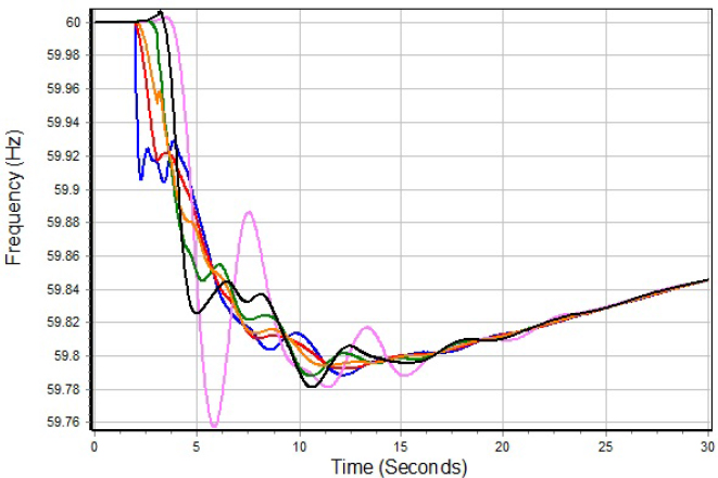
Within North America, TS cases are available for all four major interconnects.⁴ Large-scale studies done for the Western Interconnection and the Electric Reliability Corporation of Texas interconnection usually include a representation of the entire interconnect, whereas for the large Eastern Interconnection (which includes the Quebec Interconnection) an equivalenced representation is often used. Typical system sizes might be up to 20,000 buses and more than 100,000 state variables. As an example, Figure 3.3 shows the bus frequencies at six locations in a large system 2 sec after a large generator outage contingency.

A TS study can be similar to CA in that a variety of different contingencies might be considered. Also like CA, such a TS study is naturally parallel since the solution of each contingency is independent of the others. On a reasonably fast PC, a single TS solution for a single contingency on a 20,000-bus system might run an order of magnitude slower than in real time.

___________________

³ “Hunting oscillation” is a self-oscillation about an equilibrium describing how a system “hunts” for equilibrium.

⁴ As with power flow, “case” is used here to refer to the power system model parameters needed to solve a transient stability. Usually the transient stability case information supplements the information provided by the power flow case, with both needed to do a transient stability study.

Transient stability studies are routinely performed for planning purposes and for next-day operational studies. Their use in real-time operations, in which the starting point would be the SE power flow case augmented with system dynamics, is in its infancy. The increasing penetration of inverter-based resources leads to concerns among some grid operators about managing inertial response and TS better operationally, so there is a need to increase such near-real-time TS assessment. While a great deal of research has been done to explore the use of direct methods for assessing stability (such as with Lyapunov functions), to date there has not been a successful formulation that can be used for realistic problems; Lyapunov-based techniques are sometimes used for screening to determine contingencies that are likely to have problems.

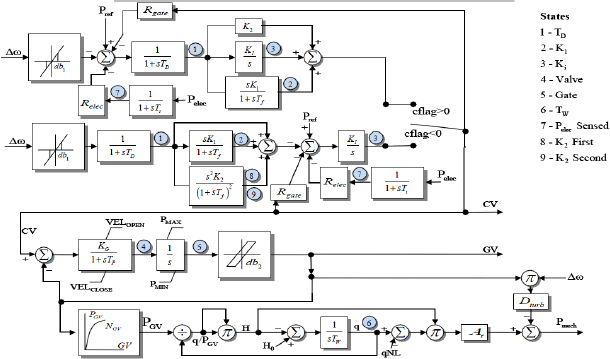
While TS data are considered more confidential than power flow data, cases can sometimes be obtained for research purposes through nondisclosure agreements. The cases can be interchanged between different software packages using several text file formats, with the formats changing slightly from software version to version. Commercial packages support on the order of several hundred different dynamic models. As an example, Figure 3.4 shows the block diagram for a nine-state hydro governor model. Models have been growing in complexity, particularly those used to represent the load. For example, now one load model requires over 100 parameters. However, there is a continued need for improved dynamic load models. This is an area in which new data-driven models based on machine learning could play a significant role.

As was the case with the power flow, one difficulty potentially impeding research is that some of the transient stability models used in systemwide studies are not publicly available. This includes proprietary user-defined models distributed only in a machine-readable format. Hence these models cannot be evaluated by the broad

power community including researchers. While the text file formats and the widely used models can be obtained by purchasing the commercial packages, the use of proprietary models and text file formats can limit access to researchers outside the power community. An example of good public availability of widely used hydro turbine-governor models and their text file descriptions for hydro generators is Koritarov et al. (2013).

Recommendation 3: The Federal Energy Regulatory Commission should require that descriptions of all models used in systemwide transient stability studies be fully public, including descriptions of any associated text file formats.

Another issue impeding research is that there are few publicly available large-scale cases. Since security concerns limit the distribution of actual system cases, an alternative would be the creation of synthetic cases with characteristics like those of the actual system; as with the power flow synthetic cases, this topic is covered more in Chapter 8.

Over the years, little work had been published on comparing the results of TS studies on the same system using different commercial packages. Such comparisons have been hindered in part because the different packages can use slightly different models. Recent work has demonstrated that quite close results could be obtained on an 18,000-bus case using two common packages (Shetye et al., 2016). However, certainly more work is needed on expanding the existing comparisons to other cases which would include different model parameters and different models, and on expanding the comparisons to other widely used packages.

Validation of the simulated results with respect to the actual system is also an important area for additional research. The models and their parameters are validated for the individual generators by disconnecting the generator from the system and then subjecting the generator to various tests to exercise its dynamics. Such testing is obviously not possible for the system itself. Rather there is a need to utilize results from the periodic disturbances that occur on the grid. Whole-system validation has also been hindered both by the lack of fast real-time measurements and the absence of dynamic models integrated with SE results. However, this is now beginning to change, driven

in part by the availability of PMU results. Load model validation differs from whole-system validation since the composition of the load is continually changing.

The advent of inverter-based resources, especially wind farms and photovoltaic farms, has greatly complicated the TS problem. The dynamics of inverter response to changed frequency and voltage can become important, especially as interconnection standards for low voltage and fault ride-through (the ability of a device to operate and remain connected to the grid while the fault is cleared) are more and more prevalent. In the case of wind farms, the dynamics of the turbine and turbine controls behind the inverter are also important. Because these technologies are developing rapidly and in some cases are manufacturers’ proprietary models, industry standard models with sufficient fidelity for TS lag behind the real-world developments (Yaramasu et al., 2015). The development of inverter-based synthetic inertia and synthetic governor response from wind farms, photovoltaic farms, and grid-connected storage systems will create additional modeling complexity.

The simulation of the system including time dynamics over longer periods of time than TS has been called mid-term stability simulation, and long-term stability simulation as the time period is extended (Kundur, 1994). Dynamic stability (DS) simulations typically simulate the generator prime mover (steam firing and steam turbine, governor, and controls) but not the electromechanical effects. In effect, DS simulations consider the TS problem with the assumption of a common single-frequency throughout, solutions over longer time periods (from hours up to a day), and with longer-term dynamics (such as prime mover fuel/combustion side effects) modeled. DS simulations can embed a power flow for a network solution or can rely on simpler representations to compute intercontrol-area interchange flows without the intra-area network representation. DS simulations are typically the basis of Operator Training Simulator real-time simulations for power system dynamics (Latimer and Masiello, 1978; Podmore et al., 1982; Prais et al., 1989) with TS solutions introduced when switching events occur.

DS solutions have become more important in recent years as a result of the increased use of renewable sources, which causes concerns about system dynamic performance in terms of frequency and area control error—control area dynamic performance. DS solutions typically rely on IEEE standard models for generator dynamics and simpler models for assumed load dynamics. As with TS solutions, providing accurate models for wind farm dynamics and for proposed synthetic inertial response and governor response is a challenge. DS solutions have also been used to investigate algorithms for incorporating fast storage into control area automatic generation control (AGC) and similar questions (Masiello and Katzenstein, 2012). Another recent trend is the incorporation of the longer-term DS dynamics into TS packages, blurring or eliminating the differences between the two.

SHORT-CIRCUIT ANALYSIS

Short-circuit calculations are a calculation of the short-circuit current and impedance visible when a fault to ground or from phase to phase is introduced in the network. Faults can be introduced at a node or along a branch. Short circuits can be single, two, or three phase, and can be phase to phase, so three-phase network models are normally utilized. While the primary purpose is to calculate the worst-case currents that will occur during a fault, it is also important to know the phase voltages during the fault. Short-circuit calculations are used in sizing circuit breakers, in analyzing the short-circuit duties of apparatus (especially transformers and generators), and in setting protection. A short-circuit calculation is a specialized load flow with a zero impedance to ground or from phase to phase inserted at the hypothesized fault location. Short-circuit analysis is generally used in transmission planning for design and protection setting; it is rarely used online, as the operating assumption is that the system is built and protected to be safe against short-circuit conditions.

ELECTROMAGNETIC TRANSIENTS

The transmission lines can be represented as a form of waveguide or transmission pipe for the purpose of assessing wave propagation down the line. At every change of impedance along the line in a network, reflections are created. As discussed in Chapter 1, switching transients, faults, and, especially, lightning strikes cause waves of voltage change to propagate along the network at near the speed of light in the medium. These step-function waves deteriorate over time and distance due to losses, but the reflections can combine and in some cases produce

voltage transients of double the nominal line voltage or more. Lightning protection such as arresters is designed to constrain the maximum overvoltage that can occur. The first digital solutions for solving electromagnetic transients date from the late 1960s with the introduction of a technique using trapezoidal integration coupled with sparsity techniques (Dommel, 1969). Electromagnetic transient analysis is used in power system engineering and planning applications.

The advent of high penetrations of inverter-based renewable generation (wind farms, solar farms) has led to a requirement for interconnection studies for each new renewable resource to ensure that the new wind farm will not create problems for the transmission system. These interconnection studies begin with load-flow analyses to ensure that the transmission system can accommodate the increased local generation, but then broaden to address issues specific to inverter-based generation, such as analyzing harmonic content and its impact on the balanced three-phase system.

HARMONIC ANALYSIS

The models described in all sections of this report are based on the 60-Hz waveform and the assumption that the waveform is “perfect,” meaning that there are no higher-order harmonics caused by nonlinearities, switching, imperfect machines and transformers, and so on. However, inverters are switching a dc voltage at high frequencies to approximate a sine wave, and this inevitably introduces third, fifth, and higher-order harmonics or non-sine waveforms into the system. The increased use of renewables and also increased inverter-based loads make harmonic analysis—study of the behavior of the higher harmonics—more and more important. While interconnection standards tightly limit the harmonic content that individual inverters may introduce into the system, the presence of multiple inverter-based resources in close proximity (as with a new transmission line to a region having many wind farms) can cause interference effects among the multiple harmonic sources.

GENERATION ANALYTICS

For more than 50 years, the problem of balancing generation to load has been addressed with a series of control and decision-support tools operating at different time frames. The primary response is the autonomous operation of generator governor control in response to frequency deviation from 60 Hz so as to control frequency deviation in a coordinated way. Governor “droop” on a uniform basis across many generators ensures that each governor responds to frequency changes proportional to its size. Secondary control operating at a 2- or 4-second interval responds to the net frequency change (residual of governor action) to restore frequency to nominal. (This is called load frequency control, or LFC.) In interconnected systems, which is the norm everywhere except for systems that constitute “electrical islands,” the deviation of inter-tie flows from scheduled flows is adjusted in a coordinated way using tie-line-bias control, which uses the natural aggregate frequency response of each control area in conjunction with the tie flow deviation to allow each control area to adjust generation to meet its own load and restore frequency. The principles of tie line bias control have not changed since the 1950s, and NERC standards today govern the operation of AGC. The actual control algorithm in use in almost all control centers is a proportional integral derivative controller with more or less sophisticated logic for allocating the control signal to the generators participating in secondary control (called “regulation” in most markets/control areas). Model predictive control (MPC) has been developed extensively in the literature for the AGC problem but has rarely been applied in the field. The minor improvements in the system (which are not required by NERC standards today) do not justify the increased cost and complexity of the software and the models needed. However, high penetration by renewables, decreased conventional generation available for regulation, the advent of new technologies such as fast short-term storage (flywheels, batteries), and short-term renewable production forecasting may reopen the investigation of MPC for AGC (Masiello and Katzenstein, 2012).

Tertiary control, or real-time dispatch, occurs at slower intervals—5 minutes in most market systems, or on demand as total load changes in vertically integrated utility operations. Tertiary control, historically called economic dispatch, reallocates the total generation among online units so as to minimize production cost. This occurs when all the unconstrained generators have the same incremental cost, with this value referred to as the

system lambda and when the total generation is equal to the total load plus losses. Originally economic dispatch was solved on special analog computers (Kirchmayer, 1959). Refinements on “lambda dispatch” added a second Lagrange multiplier µ as the cost of an aggregate constraint such as total system reserve (Stadlin, 1971). This economic dispatch paradigm is still in widespread use in vertically integrated or small control areas.

In a market environment hour-ahead bids/offers for incremental/decremental generation are used as a proxy for the unit incremental cost curves used in economic dispatch. Increasingly, market operators are using a variation of the mixed integer programming scheduling solution to solve the 5-min dispatch problem as an integrated solution of current state and near-term forecast (5, 10, 15, . . . , 60 min ahead) conditions as “trajectories” for optimal dispatch. These solutions can accommodate quick-start units that can be started in near real time, short-term loads, and renewable production forecasts.

It has become apparent in recent work on the United Kingdom’s national grid that there are trade-offs among the three control domains—primary, secondary, and tertiary—in that altered performance in one causes altered requirements in the others. For example, less primary response entails more secondary response; better performing secondary response can mitigate the efforts required in the tertiary controls; and better forecasting in the “trajectory” solution will keep dispatch closer to load and place less demand on secondary response. What has not been done as yet is to unify the mathematics for these three “products” so as to enable rigorous analysis of the best portfolio for cost and reliability, as opposed to standards-based determination, especially of the first two.

The hour-ahead and day-ahead schedules, as well as simulations of annual production costing on an hourly basis, can be lumped under the domain of security-constrained unit commitment (SCUC). Dynamic programming (Larson, 1967) was first used to perform the unit commitment analysis (identifying which generators should be running at what level each hour) in the 1970s. Today, commercial SCUC solutions have migrated to the mixed integer programming (MIP) formulation for vastly increased computational performance (as described in Chapter 4). MIP also allows more flexible modeling of complex unit behavior such as multistate combined cycle plants (which have more than one combustion turbine and more than one steam turbine capable of operating in different configurations). When integrated with an OPF (usually a semilinearized or “dc” network model) the SCUC can produce nodal prices. Applications of MIP for unit scheduling include market operations; generator operator simulation of markets for bidding support; annual production costing for studying future generation portfolios; renewable penetrations; impacts of transmission planning; and generation interconnection studies, including the probability of wind curtailment for transmission constraints. Even as MIP algorithms have enabled larger and larger networks and generation fleets to be studied, the industry appetite grows faster. To perform one interconnection study, it is typical to simulate annual production cost for an entire interconnection, which can take several hours to perform.

One noteworthy point is that the commercial SCUC software tools in use today will formulate the problem in proprietary code/databases but then interface to third-party MIP engines using industry standard integration layers. The YALMIP suite is an example of this. Users can then select the MIP engine (CPLEX, for example) that best suits their problem at hand. Developers of the MIP engines focus on the performance and robustness of their particular algorithm and code.

Dynamic programming (DP) is still the algorithm of choice for generation scheduling where energy levels are a state variable linking the solution at each time step. This is typical in hydrothermal (H-T) coordination. H-T coordination has become less of an issue in the United States, where market regimes eliminate vertical decision making, but is very much an issue in other regions (Brazil, for example). An interesting question today is whether the integration of large numbers of independent storage resources with their markets will tax MIP engines and cause a revisit of the DP versus MIP decision or the development of new algorithms to adapt to large numbers of storage resources. Current market rules that force storage to participate on the same basis as generators make this question moot, but market rules may evolve to raise the issue. Conversely, the issue may itself limit the evolution of market rules around storage. Incorporating stochastic characterizations of renewable production into the SCUC formulation can lead to brute force Monte Carlo simulations or to stochastic DP formulations (LLNL, 2014). With the possible exception of long-term hydrothermal coordination codes, these are still being studied and no solutions are commercially available today.

In planning studies, generation capacity and contingency analysis studies have been focused on a probabilistic analysis of the likelihood of insufficient capacity at a given moment owing to multiple unit outages. This

loss-of-load probability (LOLP) (Billington, 1996) has become a reliability standard in long-term planning. For capacity planning today, renewable resources and demand response resources are assigned a capacity factor or de-rating for use in capacity adequacy studies and LOLP calculations. There may be a need to consider how these capacity factors can be made stochastic and integrated into the LOLP along with stochastic generator outage statistics.

MODELING HIGH-IMPACT, LOW-FREQUENCY EVENTS

An emerging area for which some analytic tools and methods are now becoming available is the modeling of what are often referred to as high-impact, low-frequency (HILF) events (NERC, 2010)—that is, events that are statistically unlikely but still plausible and, if they were to occur, could have catastrophic consequences. These include large-scale cyber or physical attacks, pandemics, electromagnetic pulses (EMPs), and geomagnetic disturbances (GMDs). This section focuses on GMDs since over the last several years there has been intense effort in North America to develop standards for assessing the impact of GMDs on the grid. Associated with the effort has been the emergence of commercial tools to help utilities carry out such assessments.

GMDs, which are caused by coronal mass ejections from the Sun, can impact the power grid by causing low-frequency (less than 0.1 Hz) changes in Earth’s magnetic field. These magnetic field changes then cause quasi-dc electric fields, which in turn cause what are known as geomagnetically induced currents (GICs) to flow in the high-voltage transmission system. The GICs impact the grid by causing saturation in the high-voltage transformers, leading to potentially large harmonics, which in turn result in both greater reactive power consumption and increased heating. It has been known since the 1940s that GMDs have the potential to impact the power grid; a key paper in the early 1980s showed how GMD impacts could be modeled in the power flow (Alberston et al., 1981). The two key concerns associated with large GMDs are that (1) the increased reactive power consumption could result in a large-scale blackout and (2) the increased heating could permanently damage a large number of hard-to-replace high-voltage transformers (NERC, 2012).

The magnitudes of GMDs are expressed in nanotesla (nT)-per-minute variations in Earth’s magnetic field.⁵ Large GMDs are quite rare but could have catastrophic impact. For example, a 500 nT/min storm blacked out Quebec in 1989. Larger storms, with values of up to 5,000 nT/min, occurred in 1859 and 1921, both before the existence of large-scale grids. Since such GMDs can be continental in size, their impact on the grid could be significant, and tools are therefore needed to predict them and to allow utilities to develop mitigation methods.

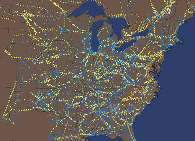
As a result of the recent effort led by NERC over the last 3 years, GMD assessment has been integrated into several commercial power analysis tools (Overbye et al., 2012). For example, GICs can be calculated for assumed uniform or nonuniform electric field variations and simultaneously their transformer impact integrated into the power flow calculations. Figure 3.5 shows the GICs calculated for an assumed uniform 2 V/km electric field over the Eastern Interconnection. More recently such calculations have also been integrated into the TS calculations, paving the way for the modeling of the much larger but shorter-time-frame GICs that could be caused by an EMP. While good progress has been made, the power system modeling of HILFs has only just begun.

___________________

⁵ A tesla (T) is a unit of magnetic induction equal to one weber per square meter; nT abbreviates nanotesla.

REFERENCES

Hughes, T.P. 1983. Networks of Power. John Hopkins University Press, Baltimore, Md. p. 43.

Iwamoto, S., and Y. Tamura. 1981. A load flow calculation for ill-conditioned power systems. IEEE Transactions on Power Apparatus and Systems PAS-100(4):1736-1743.

Kirchmayer, L.K. 1959. Differential analyzer aids design of electric utility automatic dispatching system. Transactions of the American Institute of Electrical Engineers, Part II: Applications and Industry 77(6):572-579.

Koritarov, V., L. Guzowski, J. Feltes, Y. Kazachkov, B. Lam, C. Grande-Moran, G. Thomann, L. Eng, B. Trouille, and P. Donalek. 2013. Review of Existing Hydroelectric Turbine-Governor Simulation Models. Argonne National Laboratory. ANL/DIS-13/05. August. http://ceeesa.es.anl.gov/projects/psh/ANL_DIS-3_05_Review_of_Existing_Hydro_and_PSH_Models.pdf.

Kundur, P. 1994. Power System Stability and Control. McGraw-Hill Education, New York, N.Y.

Larson, R.E. 1967. A survey of dynamic programming computational procedures. IEEE Transactions on Automatic Control 12(6):767-774.

Latimer, J.R., and R. Masiello. 1978. Design of a dispatcher training system. Abstract, 1977 Power Industry Computer Applications Conference. IEEE Transactions on Power Apparatus and Systems PAS-97(2):315.

LANL (Los Alamos National Laboratory). 2014. “Automated Demand Response and Storage for Renewable Integration.” California Energy Commission Public Workshop. June 16. Unpublished.

Masiello, R.D., and W.P. Katzenstein. 2012. “Adapting AGC to Manage High Renewable Resource Penetrations.” Power and Energy Society General Meeting. IEEE. pp. 1-6. doi:10.1109/Pesgm.2012.6345486.

NERC (North American Electric Reliability Corporation). 2010. High-Impact, Low-Frequency Event Risk to the North American Bulk Power System. June. http://www.nerc.com/pa/CI/Resources/Documents/HILF%20Report.pdf.

NERC. 2012. 2012 Special Reliability Assessment Interim Report: Effects of Geomagnetic Disturbances on the Bulk Power System. February. http://www.nerc.com/files/2012GMD.pdf.

NERC. 2015. “Standard TLP-001-4—Transmission System Planning Performance Requirements.” http://www.nerc.com/files/TPL-001-4.pdf. Accessed September 15, 2015.

Overbye, T.J., X. Cheng, and Y. Sun. 2004. “A Comparison of the ac and dc Power Flow Models for LMP Calculations.” Proceedings of the 37th Hawaiian International Conference on System Sciences.https://www.computer.org/csdl/proceedings/hicss/2004/2056/02/205620047a.pdf.

Overbye, T.J., T.R. Hutchins, K.S. Shetye, J. Weber, and S. Dahman. 2012. “Integration of Geomagnetic Disturbance Modeling into the Power Flow: A Methodology for Large-Scale System Studies.” Proceedings of the 2012 North American Power Symposium. file:///C:/Users/ cgruber/Downloads/Overbye_NAPS_GIC_2012_June1-2012.pdf.

PJM Operations Support Division. 2015. Energy Management System (EMS) Model Updates and Quality Assurance (QA). Manual M-03A. January. http://www.pjm.com/documents/manuals.aspx.

Podmore, R., J.C. Giri, M.P. Gorenberg, J.P. Britton, and N.M. Peterson. 1982. An advanced dispatcher training simulator. IEEE Transactions on Power Apparatus and Systems PAS-101:17-25.

Prais, M., G. Zhang, Y. Chen, A. Bose, and D. Curtice. 1989. Operator training simulator algorithms and test result. IEEE Transactions on Power Systems 4(3).

Sato, N., and W.F. Tinney. 1970. Techniques for exploiting the sparsity of the network admittance matrix. IEEE Transactions on Power Apparatus and Systems PAS-89:120-125.

Schweppe, F.C., and R.D. Masiello. 1971. A tracking static state estimator. IEEE Transactions on Power Apparatus and Systems 90(3):1025-1033.

Schweppe, F.C., and J. Wildes. 1974. Power system static-state estimation, Part 1: Exact model. IEEE Transactions on Power Apparatus and Systems PAS-93:859-869.

Shetye, K.S., T.J. Overbye, S. Mohapatra, Ran Xu, J.F. Gronquist, and T.L. Doern. 2016. Systematic determination of discrepancies across transient stability packages. IEEE Transactions on Power Systems 31(1):432-411.

Stadlin, W.O. 1971. Economic allocation of regulating margin. IEEE Transactions on Power Apparatus and Systems PAS-90(4):1776-1781.

Stott, B. 1979. Power system dynamic response calculations. Proceedings of the IEEE 67(2):219-241.

Stott, B., and O. Alsac. 1974. Fast decoupled load flow. IEEE Transactions on Power Apparatus and Systems PAS-93(3):859-869.

Subramanian, A.K., and J. Wilbur. 1983. Power system security function as of the energy control center at the Orange and Rockland utilities. IEEE Transactions on Power Apparatus and Systems PAS-102(12):3825-3834.

Thorp, J.S., and S.A. Naqavi. 1989. “Load Flow Fractals.” Proceedings of the 28th IEEE Conference on Decision and Control. doi:10.1109/ CDC.1989.70472.

Tinney, W.F., and C.E. Hart. 1967. Power flow solution by Newton’s method. IEEE Transactions on Power Apparatus and Systems PAS-86(11):1449-1460.

Working Group on a Common Format for Exchange of Solved Load Flow Data. 1973. Common format for exchange of solved load flow data. IEEE Transactions on Power Apparatus and Systems PAS-92(6):1916-1925.

Yaramasu, V., B. Wu, P. Sen, S. Kouro, and M. Naraimani. 2015. High-power wind energy conversion systems: State-of-the-art and emerging technologies. Proceedings of the IEEE 103(5):740-788.

REFERENCES

Albertson, V.D., J.G. Kappenman, N. Mohan, and G.A. Skarbakka. 1981. Load-flow studies in the presence of geomagnetically-induced currents. IEEE Transactions on Power Apparatus and Systems 100(2):594-607.
Alsac, O., and B. Stott. 1974. Optimal load flow with steady-state security. IEEE Transactions on Power Apparatus and Systems PAS-93(3):745-751. Billington, R.A. 1996. Reliability Evaluation of Power Systems, 2nd ed. Springer, New York, N.Y.
Brown, R.J., and W.F. Tinney. 1957. Digital solutions for large power networks. Transactions of the American Institute of Electrical Engineers, Part III: Power Apparatus and Systems 76: 347-351.
Castillo, A., and R.P. O’Neill. 2013. “Survey of Approaches to Solving the ACOPF.” U.S. Federal Energy Regulatory Commission. March. http://www.ferc.gov/industries/electric/indus-act/market-planning/opf-papers/acopf-4-solution-techniques-survey.pdf.
DeMarco, C.L., and T.J. Overbye. 1988. Low voltage power flow solutions and their role in exit time bases security measure for voltage collapse. Pp. 2127-2131 in Proceedings of the 27th IEEE Conference on Decision and Control. doi:10.1109/CDC.1988.194709.
Dommel, H.W. 1969. Digital computer solution of electromagnetic transients in single- and multiphase networks. IEEE Transactions on Power Apparatus and Systems PAS-88(4):388-399.
Dommel, H.W., and W.F. Tinney. 1968. Optimal power flow solutions. IEEE Transactions on Power Apparatus and Systems PAS-87(10):1866-1876.
Dyrkacz, M.S., C.C. Young, and F.J. Maginniss. 1960. A digital transient stability program including the effects of regulator, exciter and governor response. Transactions of the American Institute of Electrical Engineers, Part III: Power Apparatus and Systems 79(3):1245-1254.
El-Abiad, A.H., and G.W. Stagg. 1962. Automatic evaluation of power system performance—Effects of line and transformer outages. Transactions of the American Institute of Electrical Engineers, Part III: Power Apparatus and Systems 81(3):712-715.
FERC (Federal Energy Regulatory Commission). 2010. Form No. 715 Instructions. January. http://www.ferc.gov/docs-filing/forms/form-715/instructions.asp#Part 2.